Error analysis of nonconforming and mixed FEMs for second-order linear non-selfadjoint and indefinite elliptic problems

Abstract

The state-of-the art proof of a global inf-sup condition on mixed finite element schemes does not allow for an analysis of truly indefinite, second-order linear elliptic PDEs. This paper, therefore, first analyses a nonconforming finite element discretization which converges owing to some a  priori $L^{2}$ error estimates even for reduced regularity on non-convex polygonal domains. An equivalence result of that nonconforming finite element scheme to the mixed finite element method (MFEM) leads to the well-posedness of the discrete solution and to a priori error estimates for the MFEM. The explicit residual-based a posteriori error analysis allows some reliable and efficient error control and motivates some adaptive discretization which improves the empirical convergence rates in three computational benchmarks.

1 Introduction

The general second-order linear elliptic PDE on a simply-connected bounded polygonal Lipschitz domain $\Omega\subset{\mathbb{R}}^{2}$ with boundary $\partial\Omega$ reads for given right-hand side $f\in L^{2}(\Omega)$ as

$$\mathcal{L}u:=-\nabla\cdot(\mathbf{A}\nabla u+u{\mathbf{b}})+\gamma\>u=f\hskip 14.22636pt\mbox{in}~{}\Omega\;\;\;\;\;u=0\hskip 14.22636pt\mbox{on}~{}\partial\Omega.$$ (1.1)

The coefficients are all essentially bounded functions and the eigenvalues of the symmetric matrix ${\mathbf{A}}$ are all positive and uniformly bounded away from zero. The point is that the convective term ${\bf{b}}$ and the reaction term $\gamma$ may be arbitrary as long as the boundary value problem (1.1) is well-posed in the sense that zero is not an eigenvalue. In other words, $\mathcal{L}:H^{1}_{0}(\Omega)\to H^{-1}(\Omega)$ is supposed to be injective, where $H^{-1}(\Omega)$ is the dual space of $H^{1}_{0}(\Omega):=\{v\in H^{1}(\Omega):v|_{\partial\Omega}=0\}.$ Since $\mathcal{L}$ is a bounded linear operator between Hilbert spaces, this is equivalent to assume that $\mathcal{L}$ is an isomorphism.

It is known since schatz for conforming finite element discretization and it will be proved in this paper for nonconforming and for mixed finite element methods that sufficiently fine triangulations allow for unique discrete solution. One key argument in the proof is some representation formula for the lowest-order Raviart-Thomas solution to (1.1) in terms of the Crouzeix-Raviart solution. This circumvents the extra conditions on the coefficients from CHZ to deduce the solvability of the mixed finite element scheme and, thereby, allows a numerical analysis of the general linear indefinite problem at hand. The a priori error analysis shows a quasi-optimal error estimate by best-approximation errors.

The robust a posteriori error control is feasible for sufficiently fine (although unstructured but shape-regular) meshes on the basis of some a priori $L^{2}$ control for the nonconforming FEM by duality. This allows for reliable and efficient error estimates in terms of the explicit residual-based error estimators up to generic constants and data approximation errors.

This paper is devoted to another approach to generalized saddle-point problems via an explicit equivalence to nonconforming finite element schemes for general second-order linear indefinite and non-symmetric elliptic PDEs. The standard generalization of the Brezzi splitting lemma Brezzi to more general possibly non-symmetric bilinear forms in CHZ formulates various conditions on several boundedness and inf-sup constants. Those are essentially sufficient conditions and not equivalent to well-posedness. Observe that all conditions in CHZ hold as well for some bilinear form which involves a homotopy parameter $\lambda$ which takes away the non-symmetry or indefiniteness for $\lambda=0$ and equals the bilinear form considered in CHZ for $\lambda=1$. For such a homotopy and certain critical values of $0<\lambda<1$, the underlying PDE may have a zero eigenvalue, while the sufficient condition of CHZ is convex in $\lambda$ and so holds for that critical value as well. This illustrates that we may encounter some general second-order linear PDE, where the conditions in CHZ do not guarantee any well-posedness of the continuous or the discrete situation, while the continuous problem is well-posed, and hence, some novel mathematical ideas are required to ensure the solvability of the discrete solution in MFEM and their uniform boundedness a priori for small meshes.

This paper assumes that the parameters in the general second-order linear elliptic PDE are such that the associated boundary value problem is well-posed on the continuous level and shows with arguments like those in schatz for the conforming case that there exists discrete solutions for a first-order nonconforming finite element method provided the mesh is sufficiently fine. Based on general conforming companions as part of the novel medius analysis, which utilizes mathematical arguments between a  priori and a posteriori analysis, this paper proves $L^{2}$ error and piecewise $H^{1}$ error estimates.

The remaining parts of the paper are organized as follows. Section 2 introduces the weak and mixed weak formulations and equivalence of primal and mixed methods. Section 3 presents the Crouzeix-Raviart nonconforming finite element methods (NCFEM) and discusses the solvability of the discrete problem and the related a priori and a posteriori error estimates. Section 4 focuses on Raviat-Thomas mixed finite element methods (RTFEM), the representation of RTFEM solution via NCFEM, and a priori error estimates for RTFEM. Section 5 establishes a posteriori error estimates for the discrete mixed formulation and its efficiency. Numerical experiments in Section 6 concern to sensitivity of the a priori and a postriori error bounds and study the performance of the related adaptive algorithms.

This section concludes with some notation used through out this paper. An inequality $A\lesssim B$ abbreviates $A\leq CB$, where $C>0$ is a mesh-size independent constant that depends only on the domain and the shape of finite elements; $A\approx B$ means $A\lesssim B\lesssim_{\textbullet}A$. Standard notation applies to Lebesgue and Sobolev spaces and $\lVert\cdot\rVert$ abbreviates $\lVert\cdot\rVert_{L^{2}(\Omega)}$ with $L^{2}$ scalar product $(\cdot,\cdot)_{L^{2}(\Omega)}.$ Let $H^{m}(\Omega)$ denote the Sobolev spaces of order $m$ with norm given by $\lVert\cdot\rVert_{m}.$ The space of $\mathbb{R}^{2}$-valued $L^{2}$ and $H^{1}$ functions defined over the domain $\Omega$ is denoted by $L^{2}(\Omega;\mathbb{R}^{2})$ and $H^{1}(\Omega;\mathbb{R}^{2})$ respectively. Let $H(\text{div},\Omega)=\{{\bf q}\in L^{2}(\Omega;\mathbb{R}^{2}):\>\text{div}~{}{\bf q}\in L^{2}(\Omega)\}$ with the norm $~{}\lVert\cdot\rVert_{H(\text{div},\Omega)}$ and its dual space $H(\text{div},\Omega)^{*}.$

2 On Weak and Mixed Formulations

This section introduces the minimal assumptions, the weak formulation with a reference to solvability, and the mixed formulation for the problem (1.1) and their equivalence. Define the bilinear form $a(\cdot,\cdot)$ for $u,v\in H^{1}_{0}(\Omega)$ by

$$a(u,v)=(\mathbf{A}\nabla u+u{\mathbf{b}},\nabla v)_{L^{2}(\Omega)}+(\gamma\>u,v)_{L^{2}(\Omega)}.$$

The weak formulation of (1.1) reads: Given $f\in{L^{2}(\Omega)},$ seek a function $u\in H^{1}_{0}(\Omega)$ such that

$$a(u,v)=(f,v)_{L^{2}(\Omega)}\qquad\mbox{for all}\;v\in H^{1}_{0}(\Omega).$$ (2.1)

Throughout this paper, the following assumptions (A1)-(A2) are posed on the coefficients and solution of the problem (1.1).

1. The coefficient matrix $\mathbf{A}\in L^{\infty}(\Omega;\mathbb{R}_{sym}^{2\times 2})$ is positive definite; that is, there exist positive numbers $\alpha$ and $\varLambda$ such that $\alpha|{\bm{\xi}}|^{2}\leq\mathbf{A}(x){\bm{\xi}}\cdot{\bm{\xi}}\leq\varLambda|{\bm{\xi}}|^{2}$ for $\text{a.e.}~{}x\in\Omega$ and for all ${\bm{\xi}}\in\mathbb{R}^{2}$. Further, the coefficient matrix ${\bf A}$, vector ${\bf b}$ and $\gamma$ are Lipschitz continuous.

2. Given any $f\in L^{2}(\Omega)$, the problem (1.1) has a unique weak solution $u\in H^{1}_{0}(\Omega).$

The dual problem reads: Given $g\in L^{2}(\Omega)$, seek a solution $\Phi\in H^{1}_{0}(\Omega)$ such that

$$a(v,\Phi)=(g,v)_{L^{2}(\Omega)}\qquad\mbox{for all}\;v\in H^{1}_{0}(\Omega).$$ (2.2)

The unique solvability of (2.2) follows by duality from the well-posedness of $\mathcal{L}$, in (A2) and, as a consequence, $\lVert\Phi\rVert_{1}\leq C\lVert g\rVert.$

1. Suppose that there exist some constants $0<\delta<1$ and $C(\delta)<\infty$ such that the unique solution $\Phi=\mathcal{L}^{-1}g$ of (2.2) satisfies $\Phi\in H^{1+\delta}(\Omega)\cap H^{1}_{0}(\Omega)$ and

   $$\|\Phi\|_{1+\delta}\leq C(\delta)\|g\|.$$ (2.3)

Since $0$ is not part of the spectrum of $\mathcal{L}$, the Fredholm alternative (evans, , Theorem 5 pp. 305-306) proves that the problem (1.1) has a unique weak solution for each $f\in L^{2}(\Omega).$ For more detailed information on existence and uniqueness result of the weak solution to (1.1) or to (2.2), see (GT, , Theorem 8.3 pp. 181-182) or (evans, , Theorem 4 pp. 303-305). For (2.3), refer to (dauge, , cf. $\S$ 5.e and $\S$ 14.A).

Introduce new variables ${\bf p}=-({\mathbf{A}\nabla u+u{\mathbf{b}}})$ and ${\mathbf{b}}^{*}=\textbf{A}^{-1}{\bf b}$ and rewrite (1.1) as a first-order system

$$\begin{array}[]{lll}\mathbf{A}^{-1}{\bf p}+u{\mathbf{b}}^{*}+\nabla u=0\;~{}{\text{and}}~{}~{}{\text{div}}~{}{\bf p}+\gamma\>u=f\;{\rm in}\;\Omega.\end{array}$$ (2.5)

The mixed formulation seeks $({\bf p},u)\in H(\text{div},\Omega)\times L^{2}(\Omega)$ such that

$$\begin{array}[]{llll}(\textbf{A}^{-1}{\bf p}+u{\bf b}^{*},{\bf q})_{L^{2}(\Omega)}-({\rm div}~{}{\bf q},u)_{L^{2}(\Omega)}=0\qquad\mbox{for all}\;{{\bf q}}\in H(\text{div},\Omega),\\ ({\text{div}}~{}{\bf p},v)_{L^{2}(\Omega)}+(\gamma\>u,v)_{L^{2}(\Omega)}=(f,v)_{L^{2}(\Omega)}\qquad\qquad\mbox{for all}\;v\in L^{2}(\Omega).\end{array}$$ (2.8)

Theorem 2.1

(Equivalence of primal and mixed formulation)  The pair $({\bf p},u)\in$ $H(\text{\rm div},\Omega)\times L^{2}(\Omega)$ solves (2.8) if and only if $u\in H^{1}_{0}(\Omega)$ solves (1.1) and
${{\bf p}}=-({\textbf{A}\nabla u+u{\mathbf{b}}}).$

Proof. Let $({\bf p},u)\in H(\text{div},\Omega)\times L^{2}(\Omega)$ solve (2.8) and let $\phi\in{\cal D}(\Omega).$ Since ${\bf q}:=\text{Curl}~{}\phi:=(-\partial\phi/\partial x_{2},\partial\phi/\partial x_{1})$ is divergence-free and an admissible test function in the first equation of (2.8), a formal integration by parts with $\rm{curl}~{}$ defined for any smooth vector field ${\bf r}=(r_{1},r_{2})$ by $\rm{curl}~{}{\bf r}:=\partial r_{1}/\partial x_{2}-\partial r_{2}/\partial x_{1}$ proves

$$\text{curl}~{}(\textbf{A}^{-1}{\bf p}+u{\bf b}^{*})=0\;\text{in}\;{\cal D}^{\prime}(\Omega).$$

The Helmholtz decomposition shows for the simply-connected domain $\Omega$ that $A^{-1}{\bf p}+u{\bf b}^{*}$ is the gradient of some $v\in H^{1}_{0}(\Omega)$, namely;

$$\textbf{A}^{-1}{\bf p}+u{\bf b}^{*}=\nabla v.$$

The substitution of this in the first equation of (2.8) followed by an integration by parts shows

$$(\text{div}~{}{\bf q},v+u)_{L^{2}(\Omega)}=0\qquad\text{for all }{\bf q}\in H(\text{div},\Omega).$$

It is known that the divergence operator $\text{div}:H(\text{div},\Omega)\to L^{2}(\Omega)$ is surjective and so the preceding identity proves $u+v=0$. (A direct proof follows with the test function ${\bf q}=\nabla\psi$ for the solution $\psi\in H^{1}_{0}(\Omega)$ of the Poisson problem $-\Delta\psi=u+v$ in $\Omega$.) This implies $u\in H^{1}_{0}(\Omega)$ and

$$\textbf{A}^{-1}{\bf p}+u{\bf b}^{*}=-\nabla u.$$ (2.9)

This identity is recast into ${\bf p}=-(\textbf{A}\nabla u+u{\bf b})$ so that the second equation of (2.8) leads to (1.1).

Conversely, let $u$ be a solution of (1.1) and define ${\bf p}:=-(\textbf{A}\nabla u+u{\bf b)}\in L^{2}(\Omega;\mathbb{R}^{2})$. Then (1.1) reads

$$\text{div }{\bf p}+\gamma\>u=f\quad\text{in }{\cal D}^{\prime}(\Omega).$$

Since $f-\gamma\>u\in L^{2}(\Omega)$, this implies ${\bf p}\in H(\text{div},\Omega)$ and the previous identity leads to

$$\text{div }{\bf p}+\gamma\>u=f\quad\text{a.e. in }\Omega.$$

Now, an immediate consequence is the second identity in (2.8).

The definition of ${\bf p}$ is equivalent to (2.9). The multiplication of (2.9) with any ${\bf q}\in H(\text{div},\Omega)$ followed by an integration over the domain $\Omega$ leads on the right-hand side to the $L^{2}(\Omega)$ product of $-\nabla u$ and ${\bf q}$. That term allows for an integration by parts and so leads to the first identity in (2.8). This concludes the proof. ∎The well-posedness of (1.1) states that ${\mathcal{L}}:H^{1}_{0}(\Omega)\rightarrow H^{-1}(\Omega)$ is bounded and has a bounded inverse. This is an assumption on the coefficients which excludes zero eigenvalues in the Fredholm alternative, see (GT, , Section 8.2). The system (1.1) is equivalent to (2.8) which implies that the operator

$${\mathcal{M}}:\left\{\begin{array}[]{l l}H(\text{div},\Omega)\times L^{2}(\Omega)\rightarrow H(\text{div},\Omega)^{*}\times L^{2}(\Omega),\\ ({\bf q},v)\mapsto(\textbf{A}^{-1}{\bf q}+v\textbf{b}^{*}+\nabla v,~{}\text{div}~{}{\bf q}+\gamma v)\end{array}\right.$$ (2.12)

has a range which includes $\{0\}\times L^{2}({\Omega})$; that is, for any $f\in L^{2}({\Omega})$ there exists $\mathcal{M}^{-1}(0,f),$ which solves (2.8) with the zero right-hand side in the first equation of (2.8). The a posteriori error analysis relies on the well-posedness of the operator $\mathcal{M}$ even with a general right-hand side ${\bf g}\in H(\text{div},\Omega)^{*}$ in the first equation of (2.8).

Theorem 2.2

(Well-posedness of mixed formulation)  The linear operator $\mathcal{M}$ from (2.12) is bounded and has a bounded inverse.

Proof. The injectivity follows from that of $\mathcal{L}$ and the equivalence of (1.1) and (2.8) in Theorem 2.1 for ${\bf g}=0.$ The more delicate surjectivity follows in several steps. The step one is that for ${\bf g}=0$ and any $f\in L^{2}(\Omega)$, there exists some unique $\mathcal{M}^{-1}(0,f)$ in (2.12), because of the equivalence of (1.1) and (2.8).

In step two, let ${\bf g}=\nabla v$ be the gradient of some Sobolev function $v\in H^{1}_{0}(\Omega),$ i.e.,

$$<{\bf g},{\bf q}>_{H(\text{div},\Omega)^{*}\times H(\text{div},\Omega)} = \int_{\Omega}\nabla v\cdot{\bf q}\;dx$$

$$= -\int_{\Omega}v~{}\text{div}~{}{\bf q}\;dx~{}~{}\mbox{for all}\;~{}{\bf q}\in H(\text{div},\Omega).$$

Then, $\mathcal{M}({\bf p},u)=({\bf g},f)$ is equivalent to

$${\bf p}=\textbf{A}\nabla(v-u)-u\textbf{b}\;\;{\text{and }}\;\;\text{div}~{}{\bf p}+\gamma u=f.$$

The substitution of ${\bf p}$ in the second equation shows

$$-\text{div}(\mathbf{A}\nabla u+u{\mathbf{b}})+\gamma u=f-\text{div}\,(\mathbf{A}\nabla v)\in H^{-1}(\Omega).$$

Since equation (1.1) has a unique weak solution for a given right-hand side in $H^{-1}(\Omega)$ (from (A2) and the Fredholm alternative), the previous equation has unique solution

$$u=\mathcal{L}^{-1}(f-\text{div}\,(\mathbf{A}\nabla v)\>)\in H^{1}_{0}(\Omega).$$

Since

$${\bf p}:=\mathbf{A}\nabla(v-u)-u{\bf b}\in L^{2}(\Omega;\>\mathbb{R}^{2})$$

satisfies $\text{div}~{}{\bf p}=f-\gamma u\in L^{2}(\Omega),$ it follows ${\bf p}\in H(\text{div},\Omega).$ Altogether,

$$\mathcal{M}({\bf p},u)=(\nabla v,f).$$

In step three, let ${\bf g}\in L^{2}(\Omega;\mathbb{R}^{2})\subseteq H(\text{div},\Omega)^{*}$ and consider the Helmholtz decomposition of ${\bf g}$ in the format

$$\mathbf{A}{\bf g}=\mathbf{A}\nabla\alpha+\text{Curl}~{}\beta$$

for $\alpha\in H^{1}_{0}(\Omega)$ and $\beta\in H^{1}(\Omega)/\mathbb{R}$. This decomposition follows from the solution $\alpha$ of $-\text{div}(\mathbf{A}\nabla\alpha)=-\text{div}(\mathbf{A}{\bf g})$ and the fact that the divergence free function $\mathbf{A}({\bf g}-\nabla\alpha)$ equals a rotation in the simply-connected domain $\Omega.$

Since ${\bf g}=\nabla\alpha+\mathbf{A}^{-1}\text{Curl}~{}\beta$ and from step two, the superposition principle shows that it remains to verify that

$$\mathcal{M}({\bf p},u)=(\mathbf{A}^{-1}\text{Curl}~{}\beta,0)$$

has a unique solution. Since $\text{div}\,(\text{Curl}\,\beta)=0$, this is equivalent to

$$\mathcal{M}({\bf p}-\text{Curl}~{}\beta,u)=0$$

with the obvious solution ${\bf p}=\text{Curl}~{}\beta\in H(\text{div},\Omega)$ and $u=0.$

In step four, let ${\bf g}=\nabla v$ for some $v\in L^{2}(\Omega)$ such that

$$<{\bf g},{\bf q}>_{H(\text{div},\Omega)^{*}\times H(\text{div},\Omega)}=-\int_{\Omega}v~{}\text{div}~{}{\bf q}\,dx~{}~{}\mbox{for all}~{}{\bf q}\in H(\text{div},\Omega).$$

This generalizes the step two in the sense that $v\in L^{2}(\Omega).$ The equation $\mathcal{M}({\bf p},u)=(\nabla v,0)$ is equivalent to

$$\mathcal{M}({\bf p},u-v)=(-v\textbf{b}^{*},-\gamma v).$$

This has a unique solution $({\bf p},u-v)$ in $H(\text{div},\Omega)\times L^{2}(\Omega),$ because of step three (owing to $({\bf g},f)\in L^{2}(\Omega;\mathbb{R}^{2}\times\mathbb{R})$).

In step five, let $G\in H(\text{div},\Omega)^{*}$ with its Riesz representation ${\bf{g}}\in H(\text{div},\Omega)$ in the Hilbert space $H(\text{div},\Omega)$, i.e.,

$$\forall{\bf q}\in H(\text{div},\Omega)\qquad G({\bf q})=\int_{\Omega}({\bf g}\cdot{\bf q}+\text{div}~{}{\bf g}~{}\text{div}~{}{\bf q})\;dx.$$

Then, $\mathcal{M}({\bf p}_{1},u_{1})=({\bf g},f)$ has a unique solution $({\bf p}_{1},u_{1})$ from step three and $\mathcal{M}({\bf p}_{2},u_{2})=(-\nabla\text{div}~{}{\bf g},0)$ has a unique solution $({\bf p}_{2},u_{2})$ from step four with $v=\text{div}~{}{\bf g}\in L^{2}(\Omega).$ In conclusion, $({\bf p},u):=({\bf p}_{1}+{\bf p}_{2},u_{1}+u_{2})=\mathcal{M}^{-1}(G,f).$ This concludes the proof. ∎

3 Non-Conforming Finite Element Methods

This section describes the Crouzeix-Raviart non-conforming finite element methods (NCFEM) for the problem (2.1) and discusses a priori error estimates.

3.1 Regular Triangulation

Let $\mathcal{T}$ be a regular triangulation of the bounded simply-connected polygonal Lipschitz domain ${\Omega}\subset{\mathbb{R}}^{2}$ into triangles such that $\cup_{T\in\mathcal{T}}T=\overline{\Omega}.$ Let $\mathcal{E}$ denote the set of all edges in $\mathcal{T}$, ${\mathcal{E}}({\partial\Omega})$ denote the set of all boundary edges in $\mathcal{T}$ and let $\mathcal{N}$ denote the set of vertices in $\mathcal{T}.$ Let $\text{mid}(E)$ denote the midpoint of the edge $E$ and $\text{mid}(T)$ denote the centroid of the triangle $T.$ The set of edges of the element $T$ is denoted by ${\mathcal{E}}(T).$ Let $h_{T}$ denote the diameter of the element $T\in\mathcal{T}$ and $h_{\mathcal{T}}\in P_{0}(\mathcal{T})$ the piecewise constant mesh-size, $h_{\mathcal{T}}|_{T}:=h_{T}$ for all $T\in\mathcal{T}$ with $h:=\max_{T\in\mathcal{T}}h_{T}.$ Let $|E|$ be the length of the edge $E\in\mathcal{E}$ with unit outward normal $\nu_{E}.$
Let $\Pi_{0}$ be the $L^{2}$ projection onto $P_{0}(\mathcal{T})$ and define $osc(f,\mathcal{T}):=\lVert h_{\mathcal{T}}(1-\Pi_{0})f\rVert,$ where

$$P_{r}(\mathcal{T})=\{v\in L^{2}(\Omega):\forall T\in\mathcal{T},v|_{T}\in P_{r}(T)\}.$$

Here and throughout this paper, $P_{r}(T)$, denotes the algebraic polynomials of total degree at most $r\in\mathcal{N}$ as functions on the triangle $T\in\mathcal{T}.$ The $P_{1}$ conforming finite element space reads

$$V(\mathcal{T}):=P_{1}(\mathcal{T})\cap H^{1}_{0}(\Omega).$$

The jump of ${\bf q}$ across $E$ is denoted by $[{\bf q}]_{E}$; that is, for two neighboring triangles $T_{+}$ and $T_{-},$

$$[{\bf q}]_{E}(x):=({\bf q}|_{T_{+}}(x)-{\bf q}|_{T_{-}}(x))~{}\text{ for }~{}x\in E=\partial T_{+}\cap\partial T_{-}.$$

The sign of $[{\bf q}]_{E}$ is defined by the convention that there is a fixed orientation of $\nu_{E}$ pointing outside of $T_{+}.$ Let $H^{m}(\mathcal{T})$ be the broken Sobolev space of order $m$ with broken Sobolev norm

$$\|\cdot\|_{H^{m}(\mathcal{T})}:=\left(\sum_{T\in\mathcal{T}}\|\cdot\|^{2}_{H^{m}({T})}\right)^{1/2}.$$

The piecewise gradient $\nabla_{NC}:H^{1}(\mathcal{T})\longrightarrow L^{2}(\Omega;{\mathbb{R}}^{2})$ acts as $\nabla_{NC}{v}|_{T}=\nabla v|_{T}\;\;\;\text{for all}~{}T\in\mathcal{T}.$ The broken Sobolev norm $\left|\!\left|\!\left|\cdot\right|\!\right|\!\right|_{NC}$ abbreviates $(\mathbf{A}\nabla_{NC}~{}\cdot,\nabla_{NC}~{}\cdot)_{L^{2}(\Omega)}^{1/2}$ based on an underlying triangulation $\mathcal{T}.$

3.2 Crouzeix-Raviart Non-Conforming Finite Element Methods

This subsection defines the non-conforming finite element spaces and discusses the solvability of the discrete problem and the related a priori error estimates.

Given $\displaystyle P_{1}(\mathcal{T})$, the non-conforming Crouzeix-Raviart (CR) finite element space reads

$$CR^{1}(\mathcal{T}):=\{v\in P_{1}(\mathcal{T}):\forall E\in\mathcal{E},~{}v~{}\text{ is continuous at mid($E$) }\},$$

$$CR^{1}_{0}(\mathcal{T}):=\{v\in CR^{1}(\mathcal{T}):v(\text{mid}(E))=0~{}~{}\text{for all}~{}E\in\mathcal{E}({\partial\Omega})\}.$$

Let

$$a_{NC}(w_{CR},v_{CR}):= \displaystyle\sum_{T\in\mathcal{T}}\int_{T}\Big{(}\left(\mathbf{A}\nabla w_{CR}+w_{CR}{\bf b}\right)\cdot\nabla v_{CR}+\gamma\,{w}_{CR}v_{CR}\Big{)}\;dx$$

$$= (\mathbf{A}\nabla_{NC}{w}_{CR}+{w}_{CR}{\bf b},\nabla_{NC}v_{CR})_{L^{2}(\Omega)}+(\gamma\,{w}_{CR},v_{CR})_{L^{2}(\Omega)}.$$ (3.1)

The nonconforming finite element method for (2.1) seeks ${u}_{CR}\in CR^{1}_{0}(\mathcal{T})$ such that

$$a_{NC}(u_{CR},v_{CR})=(f,v_{CR})\;\;\;\;\;\text{for all}~{}v_{CR}\in CR^{1}_{0}(\mathcal{T}).$$ (3.2)

Note that, $a_{NC}(v,w)=a(v,w)\;\;\;\text{for}\;v,w\in H^{1}(\Omega).$ Observe that there are positive constants $\alpha_{A}$ and $M_{A}$ such that

$$\alpha_{A}\|v\|^{2}_{H^{1}(\mathcal{T})}\leq\left|\!\left|\!\left|v\right|\!\right|\!\right|^{2}_{NC}\leq M_{A}\|v\|_{H^{1}(\mathcal{T})}^{2}\;\;\;\;\text{for all}~{}v\in H^{1}_{0}(\Omega)+CR^{1}_{0}(\mathcal{T}).$$

The assumptions (A1) implies that, the bilinear form $a_{NC}(\cdot,\cdot)$ satisfies the following properties (i)-(ii).
(i) Boundedness. There exists a positive constant $M$ such that

$$|a_{NC}(v,w)|\leq M\left|\!\left|\!\left|v\right|\!\right|\!\right|_{NC}\;\left|\!\left|\!\left|w\right|\!\right|\!\right|_{NC}\;\;\;\;\;\text{for all}~{}v,w\in H^{1}_{0}(\Omega)+CR^{1}_{0}(\mathcal{T}).$$ (3.3)

(ii) Gårding-type inequality. There is a positive constant $\alpha$ and a nonnegative constant $~{}~{}~{}~{}~{}~{}~{}\beta$ such that

$$\alpha\left|\!\left|\!\left|v\right|\!\right|\!\right|^{2}_{NC}-\beta\|v\|^{2}\leq a_{NC}(v,v)\;\;\;\;\;\text{for all}~{}v\in H^{1}_{0}(\Omega)+CR^{1}_{0}(\mathcal{T}).$$ (3.4)

3.3 Existence and Uniqueness of the Solution of NCFEM

This subsection is devoted to a discussion on the unique solvability of the discrete problem (3.2). The conforming finite element approximation $\Phi_{C}\in V(\mathcal{T})$ to the problem (2.2) seeks $\Phi_{C}\in V(\mathcal{T})$ with

$$a(v_{C},\Phi_{C})=(g,v_{C})\;\,{\rm for~{}all}\;\,v_{C}\in V({\mathcal{T}}).$$ (3.5)

A simple modification of arguments given in (schatz, , Theorem 2) leads to the following error estimate. Given any $\epsilon>0,$ there exists an $h_{1}=h_{1}(\epsilon)>0$ such that for $0<h\leq h_{1}$, if $\Phi\in H^{1}_{0}(\Omega)$ is a solution of (2.2) and $\Phi_{C}\in V(\mathcal{T})$ satisfies (3.5), then there holds

$$\lVert\Phi-\Phi_{C}\rVert\leq\epsilon\lVert\Phi-\Phi_{C}\rVert_{1},$$ (3.6)

and since $g\in L^{2}(\Omega)$,

$$\lVert\Phi-\Phi_{C}\rVert_{1}\leq\epsilon\lVert g\rVert.$$ (3.7)

The nonconforming finite element method (3.2) is well-posed even for more general right-hand sides.

Theorem 3.1

(Stability) For sufficiently small maximum mesh size $h$ and for all $f_{0}\in L^{2}(\Omega)$ and ${\bf{f}}_{1}\in L^{2}(\Omega;\mathbb{R}^{2}),$ the discrete problem

$$a_{NC}(u_{CR},v_{CR})=(f_{0},v_{CR})+({\bf{f}}_{1},\nabla_{NC}v_{CR})\;\;\;\;\;\text{for all}~{}v_{CR}\in CR^{1}_{0}(\mathcal{T}),$$ (3.8)

has a unique solution $u_{CR}\in CR^{1}_{0}(\mathcal{T})$. Furthermore, the solution is stable in the sense that

$$\left|\!\left|\!\left|u_{CR}\right|\!\right|\!\right|_{NC}\lesssim\lVert f_{0}\rVert+\lVert{\bf{f}}_{1}\rVert.$$ (3.9)

One of the key arguments in the proof of Theorem 3.1 is the following consistency condition.

Lemma 3.2

(Consistency) Let $\Phi$ be the unique solution of (2.2). For $\epsilon>0,$ there exists some $h_{2}>0$ such that for $0<h\leq h_{2}$ it holds

$$\sup_{0\neq v_{CR}\in CR^{1}_{0}(\mathcal{T})}\frac{|a_{NC}(v_{CR},\Phi)-(g,v_{CR})_{L^{2}(\Omega)}|}{\left|\!\left|\!\left|v_{CR}\right|\!\right|\!\right|_{NC}}\leq\epsilon\|g\|\;\;\text{for all}\;g\in L^{2}(\Omega).$$ (3.10)

Proof. Given $v_{CR}\in CR_{0}^{1}(\mathcal{T})$, define a conforming approximation by the averaging of the possible values (also known as the precise representation)

$$v_{1}(z):=v_{CR}^{*}(z):=\lim_{\delta\rightarrow 0}\frac{1}{|B(z,\delta)|}\int_{B(z,\delta)}v_{CR}dx$$

of the (possibly) discontinuous $v_{CR}$ at any interior node $z\in\mathcal{N},$ where $B(z,\delta)$ is a ball of radius $\delta$ at $z.$ Linear interpolation of those values defines $v_{1}\in V({\mathcal{T}})$. The second step defines $v_{2}\in P_{2}(\mathcal{T})\cap C_{0}(\Omega)$ which equals $v_{1}$ at all nodes ${\mathcal{N}}$ and satisfies

$$\int_{E}v_{CR}\,ds=\int_{E}v_{2}\,ds\quad\text{for all }E\in{\mathcal{E}}.$$

The third step adds the cubic bubble-functions to $v_{2}$ such that the resulting function $v_{3}\in P_{3}(\mathcal{T})\cap C_{0}(\Omega)$ equals $v_{2}$ along the edges and satisfies

$$\int_{T}v_{CR}\,dx=\int_{T}v_{3}\,dx\quad\text{for all }T\in{\mathcal{T}}.$$ (3.11)

An integration by parts shows

$$\int_{T}\nabla v_{CR}\,dx=\int_{T}\nabla v_{3}\,dx\quad\text{for all }T\in{\mathcal{T}}.$$ (3.12)

The approximation and stability properties of $v_{3}$ has been studied in former work of preconditioners for nonconforming FEM Brennerenrichment (called enrichment therein). This along with standard arguments also proves approximation properties and stability in the sense that

$$||h_{\mathcal{T}}^{-1}(v_{3}-v_{CR})||+\left|\!\left|\!\left|v_{3}\right|\!\right|\!\right|_{NC}\leq C_{1}\left|\!\left|\!\left|v_{CR}\right|\!\right|\!\right|_{NC}.$$ (3.13)

With (3.2), (2.2), (3.11)-(3.12) and the definition of $\Pi_{0},$ it follows that

$$a_{NC}(v_{CR},\Phi) - (g,v_{CR})_{L^{2}(\Omega)}$$

$$= ({{\mathbf{A}\nabla\Phi}},\nabla_{NC}v_{CR})_{L^{2}(\Omega)}+({\bf b}\cdot\nabla\Phi+\gamma\Phi-g,v_{CR})_{L^{2}(\Omega)}$$

$$= (\Pi_{0}{({{\mathbf{A}}\nabla\Phi)}},\nabla v_{3})_{L^{2}(\Omega)}+({\bf b}\cdot\nabla\Phi+\gamma\Phi-g,v_{CR})_{L^{2}(\Omega)}$$

$$= -((1-\Pi_{0}){({\mathbf{A}\nabla\Phi})},\nabla v_{3})_{L^{2}(\Omega)}$$

$$+((1-\Pi_{0})({\bf b}\cdot\nabla\Phi+\gamma\Phi-g),v_{CR}-v_{3})_{L^{2}(\Omega)}.$$

The Cauchy-Schwarz inequality with (3.13) yields

$$a_{NC}(v_{CR},\Phi)-(g,v_{CR})_{L^{2}(\Omega)}$$

$$~{}~{}~{}\leq\|(1-\Pi_{0}){({\mathbf{A}\nabla\Phi})}\|\>\|v_{3}\|_{1}+C_{1}{osc}({g-\gamma\Phi-{\bf b}\cdot\nabla\Phi},\mathcal{T})\left|\!\left|\!\left|v_{CR}\right|\!\right|\!\right|_{NC}.$$

This and the aforementioned stability  $\|v_{3}\|_{1}\leq C_{1}\left|\!\left|\!\left|v_{CR}\right|\!\right|\!\right|_{NC}$   prove

$$\sup_{0\neq v_{CR}\in CR^{1}_{0}(\mathcal{T})} \frac{|a_{NC}(v_{CR},\Phi)-(g,v_{CR})_{L^{2}(\Omega)}|}{\left|\!\left|\!\left|v_{CR}\right|\!\right|\!\right|_{NC}}$$ (3.14)

$$\leq C_{1}\|(1-\Pi_{0}){({\mathbf{A}\nabla\Phi})}\|+C_{1}{osc}({g-\gamma\Phi-{\bf b}\cdot\nabla\Phi},\mathcal{T}).$$

The approximation property of $\Pi_{0}$ proves that the first term on the right-hand side of (3.14) is bounded by

$$\|(1-\Pi_{0}){({\mathbf{A}\nabla\Phi})}\| \leq 2\lVert(1-\Pi_{0}){{\mathbf{A}}}\rVert_{\infty}\lVert\nabla\Phi\rVert+\lVert{\mathbf{A}}\rVert_{\infty}\lVert(1-\Pi_{0})\nabla\Phi\rVert$$ (3.15)

$$\leq 2C\lVert(1-\Pi_{0}){{\mathbf{A}}}\rVert_{\infty}\lVert g\rVert+\lVert{\mathbf{A}}\rVert_{\infty}\lVert(1-\Pi_{0})\nabla\Phi\rVert.$$

Given $\epsilon>0,$ from (3.7) there exists $h_{3}=h_{3}(\epsilon)>0$ such that for $0<h\leq h_{3}$

$$\lVert(1-\Pi_{0})\nabla\Phi\rVert\leq\lVert\Phi-\Phi_{C}\rVert_{1}\leq\frac{\epsilon}{4C_{1}\lVert\mathbf{A}\rVert_{\infty}}\lVert g\rVert,$$

and $\lVert(1-\Pi_{0}){\bf A}\rVert_{\infty}\leq\frac{\epsilon}{8CC_{1}}$. The boundedness of $\Phi\in H^{1}_{0}(\Omega)$ by $\lVert g\rVert$ shows

$$osc(g-\gamma\Phi-{\bf b}\cdot\nabla\Phi,\mathcal{T})\leq\lVert h(g-\gamma\Phi-{\bf b}\cdot\nabla\Phi)\rVert\leq C_{2}h\|g\|.$$

For $\epsilon>0$, there exists an $h_{4}>0$ such that for $0<h<h_{4},$ $osc(g-\gamma\Phi-{\bf b}\cdot\nabla\Phi,\mathcal{T})\leq\epsilon/2\lVert g\rVert$. Alltogether for $\epsilon>0$, there exists $0<h_{2}\leq\min\{h_{3},h_{4}\}$ such that (3.10) holds. This concludes the proof.∎ Proof of Theorem 3.1. The choice $v_{CR}=u_{CR}$ in (3.8), the Gårding’s inequality (3.4), and the discrete Friedrich inequality (Brenner-Scott, , pp 301) $\lVert u_{CR}\rVert\leq C_{dF}\left|\!\left|\!\left|u_{CR}\right|\!\right|\!\right|_{NC}$ imply

$$\alpha\left|\!\left|\!\left|u_{CR}\right|\!\right|\!\right|_{NC}^{2}\leq\beta\lVert u_{CR}\rVert^{2}+\Big{(}C_{dF}\lVert f_{0}\rVert+\lVert{\bf{f}}_{1}\rVert\Big{)}\left|\!\left|\!\left|u_{CR}\right|\!\right|\!\right|_{NC},$$ (3.16)

Hence,

$$\left|\!\left|\!\left|u_{CR}\right|\!\right|\!\right|_{NC}\leq\frac{C_{dF}\beta}{\alpha}\lVert u_{CR}\rVert+\frac{1}{\alpha}\Big{(}C_{dF}\lVert f_{0}\rVert+\lVert{\bf{f}}_{1}\rVert\Big{)}.$$ (3.17)

The Aubin-Nitsche duality argument allows for an estimate of $\|u_{CR}\|.$ Since $\mathcal{L}$ is an isomorphism, the dual problem (2.2) has a unique solution $\Phi\in H^{1}_{0}(\Omega),$ which satisfies $\|\Phi\|_{1}\leq C\|g\|.$ The conforming finite element solution $\Phi_{C}$ of (2.2) satisfies (3.5) for all $g\in L^{2}(\Omega).$ Since $V(\mathcal{T})\subset CR^{1}_{0}(\mathcal{T}),$ (3.8) shows for $v_{CR}=\Phi_{C}$ that

$$a_{NC}(u_{CR},\Phi_{C})=(f_{0},\Phi_{C})+({\bf{f}}_{1},\nabla_{NC}\Phi_{C}).$$ (3.18)

Elementary algebra and (3.18) show

$$(g,u_{CR})_{L^{2}(\Omega)} = a_{NC}(u_{CR},\Phi-\Phi_{C})+(g,u_{CR})_{L^{2}(\Omega)}-a_{NC}(u_{CR},\Phi)$$

$$+(f_{0},\Phi_{C})+({\bf{f}}_{1},\nabla_{NC}\Phi_{C})$$

$$\leq M\left|\!\left|\!\left|u_{CR}\right|\!\right|\!\right|_{NC}\|\Phi-\Phi_{C}\|_{1}+\Big{(}C_{dF}\lVert f_{0}\rVert+\lVert{\bf{f}}_{1}\rVert\Big{)}\lVert\Phi_{C}\rVert_{1}$$

$$+\left|\!\left|\!\left|u_{CR}\right|\!\right|\!\right|_{NC}\sup_{0\neq v_{CR}\in CR^{1}_{0}(\mathcal{T})}\frac{|a_{NC}(v_{CR},\Phi)-(g,v_{CR})_{L^{2}(\Omega)}|}{\left|\!\left|\!\left|v_{CR}\right|\!\right|\!\right|_{NC}}.$$

For $\epsilon>0$, there exists an $h_{5}=h_{5}(\epsilon)>0$ such that the first term on the right-hand side is made $\leq\frac{\alpha}{2C_{dF}M\beta}\epsilon\left|\!\left|\!\left|u_{CR}\right|\!\right|\!\right|_{NC}\lVert g\rVert$ and from Lemma 3.2, the third can be made $\leq\frac{\alpha}{2C_{dF}\beta}\epsilon\left|\!\left|\!\left|u_{CR}\right|\!\right|\!\right|_{NC}\lVert g\rVert$ . The choice of $g=u_{CR}$ proves

$$\|u_{CR}\|\leq\frac{\alpha\epsilon}{C_{dF}\beta}\left|\!\left|\!\left|u_{CR}\right|\!\right|\!\right|_{NC}+C(C_{dF}\lVert f_{0}\rVert+\lVert{\bf{f}}_{1}\rVert).$$

For $0<\epsilon<1$, (3.17) results in

$$\left|\!\left|\!\left|u_{CR}\right|\!\right|\!\right|_{NC}\lesssim\lVert f_{0}\rVert+\lVert{\bf{f}}_{1}\rVert.$$

This proves the stability estimate (3.9) under the assumption that (3.8) has a solution. The bound (3.9) implies also the uniqueness of solution of (3.8). In fact, if the linear system of equations had a non-trivial kernel, there would exist unbounded solutions in contradiction to (3.9).∎

3.4 A Priori Error Estimates for NCFEM

This subsection discusses a priori error bounds for the non-conforming finite element solution. For related estimates, see Chen . The following $L^{2}$ error control for nonconforming FEMs has been observed in (chenhoppe, , Eq. (3.6)) but is left without a proof and stated under the restrictive assumption $\gamma\geq 0$.

Theorem 3.3

($L^{2}$ and $H^{1}$ error)  Let $u\in H^{1}_{0}(\Omega)$ be the unique weak solution of (2.1), let $u_{CR}$ be the solution of (3.2). Then, for $\epsilon>0$, there exists sufficiently small mesh-size $h$ such that

$$\lVert u-u_{CR}\rVert\leq\epsilon\left|\!\left|\!\left|u-u_{CR}\right|\!\right|\!\right|_{NC}$$ (3.19)

and for $f\in L^{2}(\Omega)$

$$\left|\!\left|\!\left|u-u_{CR}\right|\!\right|\!\right|_{NC}\leq\epsilon\|f\|.$$ (3.20)

Proof. The Aubin-Nitsche duality technique for $g\in L^{2}(\Omega)$ plus (2.2) and (3.7) and some direct calculations prove, for any $v_{C}\in V(\mathcal{T})$, that

$$(g, u-u_{CR})_{L^{2}(\Omega)}$$

$$=a_{NC}(u-u_{CR},\Phi-\Phi_{C})+\Big{(}a_{NC}(u_{CR}-v_{C},\Phi)-(g,u_{CR}-v_{C})_{L^{2}(\Omega)}\Big{)}$$

$$\leq M\left|\!\left|\!\left|u-u_{CR}\right|\!\right|\!\right|_{NC}\;\|\Phi-\Phi_{C}\|_{1}$$

$$~{}~{}+\left|\!\left|\!\left|u_{CR}-v_{C}\right|\!\right|\!\right|_{NC}\,\sup_{0\neq w_{CR}\in CR^{1}_{0}(\mathcal{T})}\frac{|a_{NC}(w_{CR},\Phi)-(g,w_{CR})_{L^{2}(\Omega)}|}{\left|\!\left|\!\left|w_{CR}\right|\!\right|\!\right|_{NC}}$$

$$\leq\frac{\epsilon}{2}\left|\!\left|\!\left|u-u_{CR}\right|\!\right|\!\right|_{NC}\;\|g\|$$

$$~{}~{}+\inf_{v_{C}\in V(\mathcal{T})}\left|\!\left|\!\left|u_{CR}-v_{C}\right|\!\right|\!\right|_{NC}\sup_{0\neq w_{CR}\in CR^{1}_{0}(\mathcal{T})}\frac{|a_{NC}(w_{CR},\Phi)-(g,w_{CR})_{L^{2}(\Omega)}|}{\left|\!\left|\!\left|w_{CR}\right|\!\right|\!\right|_{NC}}.$$ (3.21)

Since Carhop

$$\inf_{v_{C}\in V(\mathcal{T})}\left|\!\left|\!\left|u_{CR}-v_{C}\right|\!\right|\!\right|_{NC}\leq C_{3}\left|\!\left|\!\left|u-u_{CR}\right|\!\right|\!\right|_{NC}$$

for sufficiently small mesh size $h$, the consistency condition (3.10) in (3.4) imply

$$(g,u-u_{CR})_{L^{2}(\Omega)}\leq\epsilon\;\left|\!\left|\!\left|u-u_{CR}\right|\!\right|\!\right|_{NC}\;\|g\|.$$

Hence,

$$\|u-u_{CR}\|=\sup_{0\neq g\in L^{2}(\Omega)}\frac{|(g,u-u_{CR})_{L^{2}(\Omega)}|}{\|g\|}\leq\epsilon\;\left|\!\left|\!\left|u-u_{CR}\right|\!\right|\!\right|_{NC}.$$ (3.22)

This concludes the proof of (3.19).
Given any $v_{C}\in V(\mathcal{T})\subset CR_{0}^{1}(\mathcal{T}),$ the Gårding-type inequality (3.4) shows

$$\alpha\left|\!\left|\!\left|u_{CR}-v_{C}\right|\!\right|\!\right|^{2}_{NC}-\beta\|u_{CR}-v_{C}\|^{2}\leq a_{NC}(u_{CR}-v_{C},u_{CR}-v_{C})$$

$$~{}~{}=a_{NC}(u-v_{C},u_{CR}-v_{C})+\Big{(}(f,u_{CR}-v_{C})_{L^{2}(\Omega)}-a_{NC}(u,u_{CR}-v_{C})\Big{)}.$$

The discrete Friedrichs inequality $\|u_{CR}-v_{C}\|\leq C_{dF}\left|\!\left|\!\left|u_{CR}-v_{C}\right|\!\right|\!\right|_{NC}$ leads to

$$\alpha\left|\!\left|\!\left|u_{CR}-v_{C}\right|\!\right|\!\right|_{NC} \leq C_{dF}\beta\|u_{CR}-v_{C}\|+M\|u-v_{C}\|_{1}$$

$$+\sup_{0\neq w_{CR}\in CR^{1}_{0}(\mathcal{T})}\frac{|a_{NC}(u,w_{CR})-(f,w_{CR})_{L^{2}(\Omega)}|}{\left|\!\left|\!\left|w_{CR}\right|\!\right|\!\right|_{NC}}.$$

Write $u-u_{CR}:=(u-v_{C})-(u_{CR}-v_{C})$ for an arbitrary $v_{C}$ in $V(\mathcal{T}).$ The preceding estimates plus triangle inequality show

$$\left|\!\left|\!\left|u-u_{CR}\right|\!\right|\!\right|_{NC} \leq \frac{C_{dF}\beta}{\alpha}\|u-u_{CR}\|+(\frac{C_{dF}\beta}{\alpha}+1+\frac{M}{\alpha})\inf_{v_{C}\in V(\mathcal{T})}\|u-v_{C}\|_{1}$$ (3.23)

$$+\frac{1}{\alpha}\sup_{0\neq w_{CR}\in CR^{1}_{0}(\mathcal{T})}\frac{|a_{NC}(u,w_{CR})-(f,w_{CR})_{L^{2}(\Omega)}|}{\left|\!\left|\!\left|w_{CR}\right|\!\right|\!\right|_{NC}}.$$

The last term is controlled with Lemma 3.2 which remains valid for $u\in H^{1}_{0}(\Omega)$ and for all $f\in L^{2}(\Omega).$
The error analysis of (schatz, , Theorem 2), shows for any $\epsilon>0,$ that there exists an $h_{6}=h_{6}(\epsilon)>0$ such that for $0<h\leq h_{6}$, the conforming finite element solution $u_{C}\in V(\mathcal{T})$ of (2.1) satisfies

$$\inf_{v_{C}\in V(\mathcal{T})}\|u-v_{C}\|_{1} \leq \|u-u_{C}\|_{1}\leq\epsilon\>\|f\|.$$ (3.24)

The combination of (3.22), (3.24) and (3.10) implies (3.20) for sufficiently small $h$. This concludes the proof. ∎

3.5 A Posteriori Error Analysis for NCFEM

This subsection is devoted to a posteriori error analysis of NCFEM with the residual

$${\mathcal{R}es}_{NC}(w):=(f,w)_{L^{2}(\Omega)}-a_{NC}(u_{CR},w)\qquad\text{for all }w\in V+CR^{1}_{0}(\mathcal{T}).$$ (3.25)

Theorem 3.4

(A posteriori error control)  Provided the mesh-size is sufficiently small, it holds

$$\left|\!\left|\!\left|u-u_{CR}\right|\!\right|\!\right|_{NC}\lesssim\lVert{\mathcal{R}es}_{NC}\rVert_{H^{-1}(\Omega)}+\min_{v\in V}\left|\!\left|\!\left|u_{CR}-v\right|\!\right|\!\right|_{NC}.$$ (3.26)

Proof. The proof utilizes the nonconforming interpolant $I_{NC}:H^{1}(\Omega)\rightarrow CR^{1}(\mathcal{T})$ defined by

$$I_{NC}v(\text{mid}(E)):=\frac{1}{|E|}\int_{E}v~{}ds~{}~{}~{}\text{for all}~{}v\in H^{1}(\Omega).$$

The Gårding’s inequality (3.4) for $e:=u-u_{CR}$ plus elementary algebra with the bilinear forms $a$ and $a_{NC}$ plus (2.1) for $v:=u-v_{4}$ with $v_{4}\in V$ and (3.2) for $v_{CR}:=I_{NC}u-u_{CR}$ shows that $w:=u-v_{4}+u_{CR}-I_{NC}u$ satisfies

$$\alpha\left|\!\left|\!\left|e\right|\!\right|\!\right|^{2}_{NC}-\beta\lVert e\rVert^{2}\leq(f,w)_{L^{2}(\Omega)}-a_{NC}(u_{CR},w)+a_{NC}(e,v_{4}-u_{CR}).$$ (3.27)

Given $v_{CR}$, design $v_{4}\in P_{4}(\mathcal{T})\cap C_{0}(\Omega)\subseteq V$ with

$$\forall~{}p\in P_{0}(\mathcal{T})~{}~{}\int_{\Omega}\nabla v_{4}\cdot p~{}dx=\int_{\Omega}\nabla v_{CR}\cdot p~{}dx,$$

$$\forall~{}w\in P_{1}(\mathcal{T})~{}~{}\int_{\Omega}v_{4}\cdot w~{}dx=\int_{\Omega}v_{CR}\cdot w~{}dx.$$

The choice of the $P_{4}$-conforming companion $v_{4}\in P_{4}(\mathcal{T})\cap C_{0}(\Omega)$ with $I_{NC}v_{4}=v_{CR}$ allows for $C_{apx}\approx 1$ with

$$\left|\!\left|\!\left|u_{CR}-v_{4}\right|\!\right|\!\right|_{NC}\leq C_{apx}\min_{v\in V}\left|\!\left|\!\left|u_{CR}-v\right|\!\right|\!\right|_{NC}.$$ (3.28)

The proof of (3.28) follows from the analogous arguments for $v_{3}$ in Lemma 3.2. (3.27) shows

$$\left|\!\left|\!\left|e\right|\!\right|\!\right|^{2}_{NC}\leq\frac{\beta}{\alpha}\lVert e\rVert^{2}+\frac{1}{\alpha}{\mathcal{R}es}_{NC}(w)+\frac{M}{\alpha}\left|\!\left|\!\left|e\right|\!\right|\!\right|_{NC}\left|\!\left|\!\left|u_{CR}-v_{4}\right|\!\right|\!\right|_{NC}$$ (3.29)

with the nonconforming residual ${\mathcal{R}es}_{NC}(w)$ of (3.25). Note that (3.2) implies

$$P_{1}(\mathcal{T})\cap C_{0}(\Omega)\subseteq CR^{1}_{0}(\mathcal{T})\subseteq{\mathcal{K}er}{\mathcal{R}es}_{NC}.$$ (3.30)

The dual norm and triangle inequality imply

$${\mathcal{R}es}_{NC}(w)={\mathcal{R}es}_{NC}(u-v_{4})\leq\left|\!\left|\!\left|{\mathcal{R}es}_{NC}\right|\!\right|\!\right|_{H^{-1}(\Omega)}(\left|\!\left|\!\left|e\right|\!\right|\!\right|_{NC}+\left|\!\left|\!\left|u_{CR}-v_{4}\right|\!\right|\!\right|_{NC}).$$

This and (3.29) prove

$$\left|\!\left|\!\left|e\right|\!\right|\!\right|^{2}_{NC}\leq\frac{2\beta}{\alpha}\lVert e\rVert^{2}+\frac{3}{\alpha^{2}}\left|\!\left|\!\left|{\mathcal{R}es}_{NC}\right|\!\right|\!\right|^{2}_{H^{-1}(\Omega)}+\big{(}\frac{2M^{2}}{\alpha^{2}}+{1}\big{)}\left|\!\left|\!\left|u_{CR}-v_{4}\right|\!\right|\!\right|^{2}_{NC}.$$

Theorem 3.3 shows ${\lVert e\rVert}\leq\frac{\alpha\epsilon}{2\beta}\left|\!\left|\!\left|e\right|\!\right|\!\right|_{NC}$ and hence, for $\epsilon>0$ with $0<\epsilon<1$, there exists a sufficiently small mesh-size $\lVert h_{\mathcal{T}}\rVert_{L^{\infty}(\Omega)}<<1$ such that (3.28) shows

$$\left|\!\left|\!\left|e\right|\!\right|\!\right|^{2}_{NC}\leq\frac{3}{\alpha^{2}}\left|\!\left|\!\left|{\mathcal{R}es}_{NC}\right|\!\right|\!\right|^{2}_{H^{-1}(\Omega)}+C_{apx}^{2}\big{(}\frac{2M^{2}}{\alpha^{2}}+{1}\big{)}\min_{v\in V}\left|\!\left|\!\left|u_{CR}-v\right|\!\right|\!\right|^{2}_{NC}.$$

This implies (3.26) and concludes the proof.∎The analysis of the residual ${{\mathcal{R}es}_{NC}}\in{H^{-1}(\Omega)}$ with the kernel property (3.30) is by now standard Car1 ; CH . With ${\bf p}_{CR}:=-(\mathbf{A}\nabla_{NC}u_{CR}+u_{CR}\mathbf{b}),$ the explicit residual-based error estimator of Car1 reads

$$\eta(\mathcal{T}):=\lVert h_{\mathcal{T}}(f-\gamma u_{CR}-\text{div}_{NC}{\bf p}_{CR})\rVert+\lVert h_{E}^{1/2}[{\bf p}_{CR}]_{E}\cdot\nu_{E}\rVert_{L^{2}(\cup E)}.$$ (3.31)

Further details are, therefore, omitted. The residual $\min_{v\in V}\left|\!\left|\!\left|u_{CR}-v\right|\!\right|\!\right|_{NC}$ is easily estimated by $v_{4}.$

Remark 3.5

The general a posteriori error control can be contrasted with (chenhoppe, , Theorem 3.1) for $\gamma\geq 0$, where normal jumps arise which do not play any role in this paper.

4 Mixed Finite Element Methods

This section discusses the lowest-order Raviart-Thomas mixed finite element formulation and its equivalence to the NCFEM solution and derives a priori error estimates for the mixed method.

4.1 Raviart-Thomas Finite Element Methods (RTFEM)

With respect to the shape-regular triangulation $\mathcal{T},$ the lowest-order Raviart-Thomas space reads

$$RT_{0}(\mathcal{T}):=\{{\bf q}\in H(\text{div},\Omega): \>\forall T\in\mathcal{T}~{}\exists{\bf c}\in\mathbb{R}^{2}~{}\exists d\in\mathbb{R}~{}\;\forall{\bf x}\in T,~{}{\bf q}({\bf x})={\bf c}+d~{}{\bf x}$$

$$\text{ and}\;~{}\forall E\in\mathcal{E}(\Omega),[{\bf q}]_{E}\cdot\nu_{E}=0\}.$$

Throughout this paper, $\mathbf{A}_{h}:=\Pi_{0}\mathbf{A}$, $\mathbf{b}_{h}:=\Pi_{0}\mathbf{b}$, ${\bf b}^{*}_{h}:=\mathbf{A}_{h}^{-1}{\bf b}_{h}$, $\gamma_{h}:=\Pi_{0}\gamma$, and $f_{h}:=\Pi_{0}f$ denote the respective piecewise constant approximations of $\mathbf{A}$,$~{}{\bf b},$ ${\bf b}^{*}$, $\gamma$ and $f$. The discrete mixed finite element problem (RTFEM) for (2.8) seeks $({\bf p_{M}},u_{M})\in RT_{0}(\mathcal{T})\times P_{0}(\mathcal{T})$ with

$$(\mathbf{A}_{h}^{-1}{\bf p_{M}}+u_{M}{\bf b}_{h}^{*},{\bf q}_{RT})_{L^{2}(\Omega)}-(\text{div}~{}{\bf q}_{RT},u_{M})_{L^{2}(\Omega)}=0~{}~{}\text{for all}\,{\bf q}_{RT}\in RT_{0}(\mathcal{T}),$$ (4.1)

$$(\text{div}~{}{\bf p_{M}},v_{h})_{L^{2}(\Omega)}+(\gamma_{h}u_{M},v_{h})_{L^{2}(\Omega)}=(f_{h},v_{h})_{L^{2}(\Omega)}~{}\text{for all}~{}v_{h}\in P_{0}(\mathcal{T}).~{}~{}~{}$$ (4.2)

4.2 Equivalence of RTFEM and NCFEM

The piecewise constant approximations ${\mathbf{A}}_{h}$ and ${\bf b_{h}}$ of $\mathbf{A}$ and ${\bf b}$ and

$$\displaystyle\tilde{u}_{M}({\bf x})=\left(1+\frac{S(T)}{4}\gamma_{h}\right)^{-1}\left(\Pi_{0}\tilde{u}_{CR}+\frac{S(T)}{4}f_{h}\right)\;\;\text{for}~{}x\in T\in\mathcal{T},$$ (4.3)

$$~{}~{}S(T)=\displaystyle{\int_{T}}({\bf x}-\text{mid}(T))\cdot\mathbf{A}^{-1}_{h}({\bf x}-\text{mid}(T))\,d{\bf x}\;\;\text{for}~{}T\in\mathcal{T},$$ (4.4)

define a modified nonconforming FEM problem

$$(\mathbf{A}_{h}\nabla_{NC}\tilde{u}_{CR}+\tilde{u}_{M}{\bf b}_{h},\nabla_{NC}v_{CR}) +(\gamma_{h}\tilde{u}_{M},v_{CR})$$ (4.5)

$$=(f_{h},v_{CR})~{}~{}~{}\text{ for all }\,v_{CR}\in CR^{1}_{0}(\mathcal{T}).$$

Theorem 4.1

(Stability) For sufficiently small mesh-size $h$, there exists a unique solution $\tilde{u}_{CR}\in CR^{1}_{0}(\mathcal{T})$ to discrete problem (4.5) with

$$\left|\!\left|\!\left|\tilde{u}_{CR}\right|\!\right|\!\right|_{NC}\lesssim\lVert{f}_{h}\rVert.$$ (4.6)

Proof. A substitution of $\tilde{u}_{M}$ in (4.5) leads to

$$\tilde{a}_{NC}(\tilde{u}_{CR},v_{CR})=(\tilde{f}_{h},v_{CR})~{}~{}\text{for all}~{}v_{CR}\in CR^{1}_{0}(\mathcal{T})\qquad$$ (4.7)

with $S(\mathcal{T})|_{T}=S(T)$ and

$$\tilde{a}_{NC}(\tilde{u}_{CR},v_{CR}) := (\mathbf{A}_{h}\nabla_{NC}\tilde{u}_{CR}+{\bf b}_{h}(1+\frac{S(\mathcal{T})}{4}\gamma_{h})^{-1}(\Pi_{0}\tilde{u}_{CR}),\nabla_{NC}v_{CR})_{L^{2}(\Omega)}$$

$$+~{}(\gamma_{h}(1+\frac{S(\mathcal{T})}{4}\gamma_{h})^{-1}(\Pi_{0}\tilde{u}_{CR}),v_{CR})_{L^{2}(\Omega)},$$

$$(\tilde{f}_{h},v_{CR})_{L^{2}(\Omega)} := (f_{h},v_{CR})_{L^{2}(\Omega)}-({\bf b}_{h}(1+\frac{S(\mathcal{T})}{4}\gamma_{h})^{-1}\frac{S(\mathcal{T})}{4}f_{h},\nabla_{NC}v_{CR})_{L^{2}(\Omega)}$$

$$~{}-(\gamma_{h}(1+\frac{S(\mathcal{T})}{4}\gamma_{h})^{-1}\frac{S(\mathcal{T})}{4}f_{h},v_{CR})_{L^{2}(\Omega)}.$$

The stiffness matrix related to (4.7) is very similar to that of (3.2) except for some data perturbation and the substitution of $\Pi_{0}\tilde{u}_{CR}$ instead of ${u}_{CR}$ in two lower-order terms. The last substitution models one-point integration, and since the variable $\tilde{u}_{CR}$ is controlled in the energy norm $\left|\!\left|\!\left|\cdot\right|\!\right|\!\right|_{NC},$ it acts as some perturbation as well. All these perturbations tends to zero as the maximal mesh-size tends to zero and hence, the existence, uniqueness and stability results may be deduced as in Subsection 3.3.

To be more specific, the choice $v_{CR}=\tilde{u}_{CR}$ in (4.7) implies

$$\left|\!\left|\!\left|\tilde{u}_{CR}\right|\!\right|\!\right|_{NC}\lesssim\;\|\tilde{u}_{CR}\|+\|\tilde{f}_{h}\|.$$ (4.8)

The Aubin-Nitsche duality argument allows for an estimate of $\|\tilde{u}_{CR}\|$. Recall that for given $g\in L^{2}(\Omega)$, $\Phi\in H^{1}_{0}(\Omega)$ is the unique solution of the dual problem $a(v,\Phi)=(g,v)$ from Subsection 3.3 and the conforming finite element solution $\Phi_{C}$ of (3.5) satisfies the estimate (3.7).

Since $V(\mathcal{T})\subset CR^{1}_{0}(\mathcal{T}),$ the choice of $v_{CR}=\Phi_{C}$ in (4.7) yields

$$\tilde{a}_{NC}(\tilde{u}_{CR},\Phi_{C})=(\tilde{f}_{h},\Phi_{C}).$$ (4.9)

An elementary algebra with (4.9) and the discrete Friedrich inequality shows

$$(g,\tilde{u}_{CR})_{L^{2}(\Omega)} = \tilde{a}_{NC}(\tilde{u}_{CR},\Phi-\Phi_{C})+(\tilde{f}_{h},\Phi_{C})+(g,\tilde{u}_{CR})_{L^{2}(\Omega)}-\tilde{a}_{NC}(\tilde{u}_{CR},\Phi)$$ (4.10)

$$\lesssim \left|\!\left|\!\left|\tilde{u}_{CR}\right|\!\right|\!\right|_{NC}\|\Phi-\Phi_{C}\|_{1}+\|\tilde{f}_{h}\|\;\|\Phi_{C}\|_{1}$$

$$+\left|\!\left|\!\left|\tilde{u}_{CR}\right|\!\right|\!\right|_{NC}\sup_{0\neq v_{CR}\in CR^{1}_{0}(\mathcal{T})}\frac{|\tilde{a}_{NC}(v_{CR},\Phi)-(g,v_{CR})|}{\left|\!\left|\!\left|v_{CR}\right|\!\right|\!\right|_{NC}}.$$

The last term on the right-hand side of (4.10) is

$$\tilde{a}_{NC}(v_{CR},\Phi)-(g,v_{CR})_{L^{2}(\Omega)}$$

$$=a_{NC}(v_{CR},\Phi)-(g,v_{CR})_{L^{2}(\Omega)}-(\nabla_{NC}v_{CR},({\mathbf{A}-\mathbf{A}_{h}})\nabla\Phi)_{L^{2}(\Omega)}$$

$$~{}~{}~{}-(v_{CR},(\mathbf{b}-\mathbf{b}_{h})\cdot\nabla\Phi+(\gamma-\gamma_{h})\Phi)_{L^{2}(\Omega)}-(v_{CR}-\Pi_{0}v_{CR},\mathbf{b}_{h}\cdot\nabla\Phi+\gamma_{h}\Phi)_{L^{2}(\Omega)}$$

$$~{}~{}~{}-\big{(}\frac{S(\mathcal{T})}{4}\gamma_{h}(1+\frac{S(\mathcal{T})}{4}\gamma_{h})^{-1}\Pi_{0}v_{CR},\mathbf{b}_{h}\cdot\nabla\Phi+\gamma_{h}\Phi\big{)}_{L^{2}(\Omega)}.$$

The Cauchy-Schwarz inequality, the approximation property of $\Pi_{0}$ and $S(T)\approx h^{2}$ lead to

$$\sup_{0\neq v_{CR}\in CR^{1}_{0}(\mathcal{T})} \frac{|\tilde{a}_{NC}(v_{CR},\Phi)-(g,v_{CR})_{L^{2}(\Omega)}|}{\left|\!\left|\!\left|v_{CR}\right|\!\right|\!\right|_{NC}}$$

$$\lesssim\sup_{0\neq v_{CR}\in CR^{1}_{0}(\mathcal{T})}\frac{|{a}_{NC}(v_{CR},\Phi)-(g,v_{CR})_{L^{2}(\Omega)}|}{\left|\!\left|\!\left|v_{CR}\right|\!\right|\!\right|_{NC}}\qquad$$

$$~{}~{}~{}+\big{(}h+\lVert{\bf A-A_{h}}\rVert_{\infty}+\lVert{\bf b-b_{h}}\rVert_{\infty}+\lVert{\gamma-\gamma_{h}}\rVert_{\infty}\big{)}\lVert\Phi\rVert_{1}.$$

Lemma 3.2, $\lVert{\bf A-A_{h}}\rVert_{\infty}\leq\epsilon,~{}\lVert{\bf b-b_{h}}\rVert_{\infty}\leq\epsilon,~{}\lVert{\gamma-\gamma_{h}}\rVert_{\infty}\leq\epsilon$ for $\epsilon>0$ and $\lVert\Phi\rVert_{1}\leq C\lVert g\rVert$ result in

$$\sup_{0\neq v_{CR}\in CR^{1}_{0}(\mathcal{T})} \frac{|\tilde{a}_{NC}(v_{CR},\Phi)-(g,v_{CR})_{L^{2}(\Omega)}|}{\left|\!\left|\!\left|v_{CR}\right|\!\right|\!\right|_{NC}}\lesssim\epsilon\lVert g\rVert.$$ (4.11)

The combination with (3.7) and (4.10)-(4.11) leads to $(g,\tilde{u}_{CR})\lesssim(\epsilon\;\left|\!\left|\!\left|\tilde{u}_{CR}\right|\!\right|\!\right|_{NC}+\|\tilde{f}_{h}\|)\;\|g\|.$ Hence, the boundedness of $\|\tilde{f}_{h}\|\lesssim\|f_{h}\|$ yields

$$\|\tilde{u}_{CR}\|\lesssim\epsilon\;\left|\!\left|\!\left|\tilde{u}_{CR}\right|\!\right|\!\right|_{NC}+\|{f}_{h}\|.$$

A substitution in (4.8) for sufficiently small $h$ results in

$$\left|\!\left|\!\left|\tilde{u}_{CR}\right|\!\right|\!\right|_{NC}\lesssim\|{f}_{h}\|.$$

Since $f_{h}=0$ shows that $\tilde{u}_{CR}=0,$ uniqueness follows. This also implies existence of the discrete solution. ∎

Theorem 4.2

(Equivalence of RTFEM and NCFEM)  Recall $\tilde{u}_{M}$ and $S(T)$ from (4.3)-(4.4) and let $\tilde{u}_{CR}\in CR^{1}_{0}(\mathcal{T})$ solve (4.5). Then

$$\tilde{\bf p}_{M}({\bf x})=-\left(\mathbf{A}_{h}\nabla_{NC}\tilde{u}_{CR}+\tilde{u}_{M}{\bf b}_{h}\right)+\left(f_{h}-\gamma_{h}\tilde{u}_{M}\right)\frac{\left({\bf x}-\text{\rm mid}(T)\right)}{2}\text{ for}~{}{\bf x}\in T\in\mathcal{T}$$ (4.12)

defines $\tilde{\bf p}_{M}\in RT_{0}(\mathcal{T})\subset H({\rm div},\Omega)$ and the pair $(\tilde{\bf p}_{M},\tilde{u}_{M})$ satisfies (4.1)-(4.2). Conversely, for any solution $(\tilde{\bf p}_{M},\tilde{u}_{M})$ in $RT_{0}(\mathcal{T})\times P_{0}(\mathcal{T})$ of (4.1)-(4.2) the solution $\tilde{u}_{CR}\in CR^{1}_{0}(\mathcal{T})$ of (4.5) satisfies (4.3) and (4.12).

Proof. Note that the continuity of the normal components on the boundaries of the triangles $T\in{\mathcal{T}}$ reflects the conformity $RT_{0}(\mathcal{T})\subset H(\text{div},\Omega).$ Given an interior edge $E$ shared by neighboring triangles $T_{+},T_{-}\in\mathcal{T}$ with unit normal $\nu_{E}$ pointing from $T_{-}$ to $T_{+}$, let $\psi_{E}$ denote the non-conforming basis function defined on an interior edge such that $\psi_{E}(\text{mid}(E))=1,$ while $~{}\psi_{E}(\text{mid}(F))=0~{}\text{for all }F\in\mathcal{E}\setminus\{E\}.$ A piecewise integration by parts shows

$$(\tilde{\bf p}_{M}, \nabla_{NC}\psi_{E})_{L^{2}(\Omega)}+(\text{div}_{NC}\>\tilde{\bf p}_{M},\psi_{E})_{L^{2}(\Omega)}=\int_{\partial T_{+}\cup\partial T_{-}}\tilde{\bf p}_{M}\cdot\nu\psi_{E}\,ds$$

$$=\int_{E}(\tilde{\bf p}_{M}|_{T_{+}}\cdot\nu|_{T_{+}}+\tilde{\bf p}_{M}|_{T_{-}}\cdot\nu|_{T_{-}})\psi_{E}\,ds=|E|[\tilde{\bf p}_{M}]\cdot\nu_{E},$$ (4.13)

where $\text{div}_{NC}v|_{T}=\text{div}~{}v|_{T}$. The definition of $\tilde{\bf p}_{M}$, (4.5) and the fact

$$\left((f_{h}-\gamma_{h}\tilde{u}_{M})\left({\bf x}-\text{mid}(T)\right)/2,\nabla_{NC}\psi_{E}\right)_{L^{2}(\Omega)}=0,$$

imply

$$(\tilde{\bf p}_{M},\nabla_{NC}\psi_{E})_{L^{2}(\Omega)}+(\text{div}_{NC}\>\tilde{\bf p}_{M},\psi_{E})_{L^{2}(\Omega)}=0.$$

Hence, (4.2) shows $|E|[\tilde{\bf p}_{M}]\cdot\nu=0.$ Since the edge $E$ is arbitrary in $\mathcal{E}(\Omega)$, $\tilde{\bf p}_{M}\in RT_{0}(\mathcal{T})\subset H(\text{div},\Omega).$ Since the distributional divergence is the piecewise one, (4.12) proves $\text{div}_{NC}~{}\tilde{\bf p}_{M}({\bf x})=f_{h}-\gamma_{h}\tilde{u}_{M}$. Hence, (4.2) is satisfied. A use of the definition of $\Pi_{0}$, an application of element-wise integration by parts, some elementary properties of elements in $RT_{0}(\mathcal{T}),\;CR^{1}_{0}(\mathcal{T})$, and (4.12) yield

$$(\mathbf{A}^{-1}_{h}\tilde{\bf p}_{M} + \tilde{u}_{M}{\bf b}^{*}_{h},~{}{\bf q}_{RT})_{L^{2}(\Omega)}-(\text{div}~{}{\bf q}_{RT},~{}\Pi_{0}\tilde{u}_{CR})_{L^{2}(\Omega)}$$

$$= (\mathbf{A}^{-1}_{h}\tilde{\bf p}_{M}+\tilde{u}_{M}{\bf b}^{*}_{h},~{}{\bf q}_{RT})_{L^{2}(\Omega)}-(\text{div}~{}{\bf q}_{RT},~{}\tilde{u}_{CR})_{L^{2}(\Omega)}$$

$$= (\mathbf{A}^{-1}_{h}\tilde{\bf p}_{M}+\tilde{u}_{M}{\bf b}^{*}_{h},~{}{\bf q}_{RT})_{L^{2}(\Omega)}+(\nabla_{NC}\tilde{u}_{CR},~{}{\bf q}_{RT})_{L^{2}(\Omega)}$$

$$= (\mathbf{A}^{-1}_{h}(f_{h}-\gamma_{h}\tilde{u}_{M})(\bullet-\text{mid}(\mathcal{T}))/2,~{}{\bf q}_{RT})_{L^{2}(\Omega)}.$$

Recall $S(\mathcal{T})|_{T}=S(T)$ and the definition of $S(T)$ from (4.4). Some algebraic calculations with ${\bf q}_{RT}\in RT_{0}(\mathcal{T})$ and $\displaystyle\int_{T}({\bf x}-\text{mid}(T))\>dx=0$ yield

$$(\mathbf{A}^{-1}_{h}\tilde{\bf p}_{M} +\tilde{u}_{M}{\bf b}^{*}_{h},~{}{\bf q}_{RT})_{L^{2}(\Omega)}-(\text{div}~{}{\bf q}_{RT},\Pi_{0}\tilde{u}_{CR})_{L^{2}(\Omega)}$$

$$=((f_{h}-\gamma_{h}\tilde{u}_{M})\mathbf{A}^{-1}_{h}(\bullet-\text{mid}(\mathcal{T}))/2),~{}(\bullet-\text{mid}(\mathcal{T}))/2\;\text{div}~{}{\bf q}_{RT})_{L^{2}(\Omega)}$$

$$=\left(\frac{S(\mathcal{T})}{4}(f_{h}-\gamma_{h}\tilde{u}_{M}),\text{div}~{}{\bf q}_{RT}\right)_{L^{2}(\Omega)}.$$

An appropriate re-arrangement shows that the pair $(\tilde{\bf p}_{M},\tilde{u}_{M})$ satisfies (4.1). This concludes the proof of the first part.
To prove the converse implication, let $(\tilde{\bf p}_{M},\tilde{u}_{M})$ in $RT_{0}(\mathcal{T})\times P_{0}(\mathcal{T})$ be some solution of (4.1)-(4.2). The discrete Helmholtz decomposition arnold states for the simply-connected domain $\Omega$ that the piecewise constant vector function $-\Pi_{0}(\mathbf{A}^{-1}_{h}\tilde{\bf p}_{M}+\tilde{u}_{M}{{\bf b}^{*}_{h}})\in P_{0}(\mathcal{T};\mathbb{R}^{2})$ equals a discrete gradient $\nabla_{NC}\alpha_{CR}$ of some nonconforming function $\alpha_{CR}\in CR^{1}_{0}(\mathcal{T})$ plus the Curl $\beta_{c}$ of some piecewise affine conforming function $\beta_{c}\in P_{1}(\mathcal{T})\cap C(\bar{\Omega});$ that is,

$$-(\Pi_{0}\mathbf{A}^{-1}_{h}\tilde{\bf p}_{M}+\tilde{u}_{M}{{\bf b}^{*}_{h}})=\nabla_{NC}\alpha_{CR}+{\text{Curl}~{}}\beta_{c}.$$

The argument to verify this is to define $\alpha_{CR}$ as the solution of a Poisson problem of a nonconforming FEM with the right-hand side $-(\tilde{\bf p}_{M}+\tilde{u}_{M}{\bf b}_{h},\mathbf{A}^{-1}_{h}\nabla_{NC}v_{CR})_{L^{2}(\Omega)}$ as a functional in $v_{CR}\in CR^{1}_{0}(\mathcal{T})$. Once $\alpha_{CR}$ is determined, the difference $\nabla_{NC}\alpha_{CR}+\Pi_{0}\mathbf{A}^{-1}_{h}\tilde{\bf p}_{M}+\tilde{u}_{M}{{\bf b}^{*}_{h}}$ is $L^{2}(\Omega)$ orthogonal onto $\nabla_{NC}CR^{1}_{0}(\mathcal{T}).$ Hence, it equals the Curl of some Sobolev functions so that Curl $\beta_{c}:=(-\frac{\partial\beta_{c}}{\partial x_{2}},\frac{\partial\beta_{c}}{\partial x_{1}})$ is piecewise constant. This concludes the proof of the above discrete Helmholtz decomposition.
Since Curl $\beta_{c}=:{\bf q}_{RT}$ is a divergence free Raviart-Thomas function, (4.1) implies

$$\lVert{\text{Curl}}~{}\beta_{c}\rVert^{2}=-(\mathbf{A}^{-1}_{h}\tilde{\bf p}_{M}+\tilde{u}_{M}{{\bf b}^{*}_{h}},{\bf q}_{RT})_{L^{2}(\Omega)}=0.$$

Consequently,

$$~{}\Pi_{0}\tilde{\bf p}_{M}=-\mathbf{A}_{h}\nabla_{NC}\alpha_{CR}-\tilde{u}_{M}{\bf b}_{h}.$$

The Raviart-Thomas function allows for div$~{}\tilde{\bf p}_{M}={\text{div}}_{NC}~{}\tilde{\bf p}_{M}\in P_{0}(\mathcal{T})$ and hence (in 2D),

$$\tilde{\bf p}_{M}=\Pi_{0}\tilde{\bf p}_{M}+({\text{div}}_{NC}~{}\tilde{\bf p}_{M})(\bullet-{\text{mid}({\mathcal{T}}))/2}.$$

The equation (4.2) is equivalent to ${\text{div}}_{NC}~{}\tilde{\bf p}_{M}=f_{h}-\gamma_{h}\tilde{u}_{M}.$ The combination of the previous identities proves (4.12) for $\tilde{u}_{CR}:=\alpha_{CR}$. A piecewise integration by parts of the product of $\tilde{\bf p}_{M}$ for (4.12) with $\nabla_{NC}v_{CR}$ leads to

$$-({\text{div}}_{NC}~{}\tilde{\bf p}_{M},v_{CR})_{L^{2}(\Omega)}=(\tilde{\bf p}_{M},\nabla_{NC}v_{CR})_{L^{2}(\Omega)}.$$

The aforementioned identities for $\Pi_{0}\tilde{\bf p}_{M}$ and ${\text{div}}_{NC}~{}\tilde{\bf p}_{M}$ show that this equals

$$-(f_{h}-\gamma_{h}\tilde{u}_{M},v_{CR})_{L^{2}(\Omega)}=-(\mathbf{A}_{h}\nabla_{NC}\alpha_{CR}+\tilde{u}_{M}{\bf b}_{h},\nabla_{NC}v_{CR})_{L^{2}(\Omega).}$$

This proves (4.5) for $\tilde{u}_{CR}\equiv\alpha_{CR}$. To verify (4.3), the identity (4.12) is substituted in (4.1) for some general

$${\bf q}_{RT}=\Pi_{0}{\bf q}_{RT}+(\text{div}_{NC}~{}{\bf q}_{RT})(\bullet-{\text{mid}}({\mathcal{T}}))/2\in RT_{0}(\mathcal{T}).$$

This shows

$$(\text{div}_{NC}~{}{\bf q}_{RT},\tilde{u}_{M})_{L^{2}(\Omega)} = (-\nabla_{NC}\tilde{u}_{CR},{\bf q}_{RT})_{L^{2}(\Omega)}+(f_{h}-\gamma_{h}\tilde{u}_{M},\frac{S(\mathcal{T})}{4}~{}{\text{div}}_{NC}~{}{\bf q}_{RT})_{L^{2}(\Omega)}.$$

A piecewise integration by parts shows $(-\nabla_{NC}\tilde{u}_{CR},{\bf q}_{RT})_{L^{2}(\Omega)}=(\tilde{u}_{CR},\text{div}_{NC}~{}{\bf q}_{RT})_{L^{2}(\Omega)}$ and hence,

$$\Big{(}\tilde{u}_{M}\Big{(}1+\gamma_{h}\frac{S(\mathcal{T})}{4}\Big{)}-\frac{S(\mathcal{T})}{4}f_{h}-\tilde{u}_{CR},~{}\text{div}~{}{\bf q}_{RT}\Big{)}_{L^{2}(\Omega)}=0.$$

Since the divergence operator is surjective from $RT_{0}(\mathcal{T})$ onto $P_{0}(\mathcal{T})$ and since the previous identity holds for all ${\bf q}_{RT}\in RT_{0}(\mathcal{T})$), it follows

$$\tilde{u}_{M}(1+\gamma_{h}\frac{S(\mathcal{T})}{4})=\frac{S(\mathcal{T})}{4}f_{h}+\Pi_{0}\tilde{u}_{CR}.$$

This is equivalent to (4.3) and concludes the proof. ∎

4.3 A Priori Error Estimates for RTFEM

This subsection establishes well-posedness of the mixed finite element method (4.1)-(4.2) and a priori error estimates for mixed formulation (2.8) via the equivalence of RTFEM and NCFEM.
The following theorem deals with the well-posedness of the mixed finite element method (4.1)-(4.2) with a more general right hand side.
For given ${\bf{g_{RT}}}\in RT_{0}(\mathcal{T})$, define ${\bf{g}}\in RT_{0}(\mathcal{T})^{*}$ by

$${\bf{g}}({\bf q}):=(\mathbf{A}_{h}^{-1}{\bf{g}}_{RT},{\bf q})_{L^{2}(\Omega)}+(\text{div}~{}{\bf g}_{RT},\text{div}~{}{\bf q})_{L^{2}(\Omega)}~{}~{}\text{for all}~{}{\bf q}\in RT_{0}(\mathcal{T}).$$ (4.14)

For $f_{h}\in P_{0}(\mathcal{T}),$ and ${\bf{g}}\in RT_{0}(\mathcal{T})^{*}$ a modified mixed finite element method reads as: seek $({\bf{p}_{M}},u_{M})\in RT_{0}(\mathcal{T})\times P_{0}(\mathcal{T})$ such that

$$(\mathbf{A}_{h}^{-1}{\bf p_{M}}+u_{M}{\bf b}_{h}^{*},{\bf q}_{RT})_{L^{2}(\Omega)}-(\text{div}~{}{\bf q}_{RT},u_{M})_{L^{2}(\Omega)}={\bf{g}}({\bf q}_{RT})\;\;\;$$

$$\hskip 187.78836pt\text{for all}~{}{\bf q}_{RT}\in RT_{0}(\mathcal{T}),$$ (4.15)

$$(\text{div}~{}{\bf p_{M}},v_{h})_{L^{2}(\Omega)}+(\gamma_{h}u_{M},v_{h})_{L^{2}(\Omega)}=(f_{h},v_{h})_{L^{2}(\Omega)}\;\;\text{for all}~{}v_{h}\in P_{0}(\mathcal{T}).$$ (4.16)

Theorem 4.3

(Stability)  For all ${\bf{g}}\in RT_{0}(\mathcal{T})^{*}$ given by (4.14) and $f_{h}\in P_{0}(\mathcal{T}),$ the modified mixed finite element problem (4.15)-(4.16) has a unique solution $({\bf{p}_{M}},u_{M})\in RT_{0}(\mathcal{T})\times\in P_{0}(\mathcal{T})$ with

$$\lVert({\bf{p}_{M}},u_{M})\rVert_{H(\text{\rm div},\Omega)\times L^{2}(\Omega)}\lesssim\lVert({\bf{g}},f_{h})\rVert_{H(\text{\rm div},\Omega)^{*}\times L^{2}(\Omega)}.$$ (4.17)

As in Subsection 4.2, the solution of modified RTFEM (4.15)-(4.16) is represented in terms of the solution of a suitable NCFEM.
Proof. Since ${\bf{g}}({\bf{q}})$ is given by (4.14), the equation (4.15) is written equivalently

$$(\mathbf{A}_{h}^{-1}({\bf p_{M}}-{\bf{g}}_{RT}) + u_{M}{\bf b}_{h}^{*},{\bf q}_{RT})_{L^{2}(\Omega)}=(\text{div}~{}{\bf q}_{RT},u_{M}+\text{\rm div}~{}{\bf{g}}_{RT})_{L^{2}(\Omega)}\;$$ (4.18)

$$\hskip 113.81102pt\text{for all}\,{\bf q}_{RT}\in RT_{0}(\mathcal{T}).$$

Since $-\Pi_{0}(\mathbf{A}_{h}^{-1}({\bf p_{M}}-{\bf{g}}_{RT})+u_{M}{\bf b}_{h}^{*})\in P_{0}(\mathcal{T};{\mathbb{R}}^{2}),$ the discrete Helmholtz decomposition states

$$-\Pi_{0}(\mathbf{A}_{h}^{-1}({\bf p_{M}}-{\bf{g}}_{RT})+u_{M}{\bf b}_{h}^{*})=\nabla_{NC}\alpha_{CR}+\rm{Curl}~{}\beta_{C}$$ (4.19)

for some nonconforming function $\alpha_{CR}\in CR_{0}^{1}(\mathcal{T})$ and some $\beta_{C}\in P_{1}(\mathcal{T})\cap C(\overline{\Omega}).$ The choice of ${\bf{q}}_{RT}=\rm{Curl}~{}\beta_{C}$ in (4.18) shows that $\rm{Curl}~{}\beta_{C}=0.$ Hence,

$$\Pi_{0}({\bf p_{M}}-{\bf{g}}_{RT})=-\Big{(}\mathbf{A}_{h}\nabla_{NC}\alpha_{CR}+u_{M}{\bf b}_{h}\Big{)}.$$

Equation (4.16) implies

$${\text{div}}_{NC}~{}({\bf p}_{M}-{\bf{g}}_{RT})=f_{h}-\gamma_{h}u_{M}-{\text{div}}_{NC}~{}{\bf{g}}_{RT}.$$ (4.20)

and

$$({\bf p}_{M}-{\bf{g}}_{RT})=\Pi_{0}({\bf p}_{M}-{\bf{g}}_{RT})+({\text{div}}_{NC}~{}({\bf p}_{M}-{\bf{g}}_{RT}))(\bullet-{\text{mid}({\mathcal{T}})})/2.$$

Hence,

$$({\bf p}_{M}-{\bf{g}}_{RT}) = -\Big{(}\mathbf{A}_{h}\nabla_{NC}\alpha_{CR}+u_{M}{\bf b}_{h}\Big{)}$$ (4.21)

$$+(f_{h}-\gamma_{h}u_{M}-{\text{div}}_{NC}~{}{\bf{g}}_{RT})(\bullet-{\text{mid}({\mathcal{T}}))/2}.$$

For all $v_{CR}\in CR_{0}^{1}(\mathcal{T}),$ the last term on the right hand-side of (4.21) is orthogonal to $\nabla_{NC}v_{CR}$ with respect to $L^{2}(\Omega)$ inner product. This leads to

$$(\mathbf{A}_{h}\nabla_{NC}\alpha_{CR}+u_{M}{\bf b}_{h},\nabla_{NC}v_{CR})=-({\bf p}_{M}-{\bf{g}}_{RT},\nabla_{NC}v_{CR}).$$

For the last term on the right-hand side, a piecewise integration with (4.20) yields

$$(\mathbf{A}_{h}\nabla_{NC}\alpha_{CR}+u_{M}{\bf b}_{h},\nabla_{NC}v_{CR}) + (\gamma_{h}u_{M},v_{CR})=(f_{h}-{\text{div}}_{NC}~{}{\bf{g}}_{RT},v_{CR}).$$ (4.22)

A substitution of (4.21) in (4.18) with ${\bf{q}}_{RT}:=\Pi_{0}{\bf{q}}_{RT}+({\text{div}}_{NC}~{}{\bf{q}}_{RT})(\bullet-{\text{mid}({\mathcal{T}})})/2$ and piecewise integration $(-\nabla_{NC}\alpha_{CR},{\bf q}_{RT})_{L^{2}(\Omega)}=(\alpha_{CR},\text{div}_{NC}~{}{\bf q}_{RT})_{L^{2}(\Omega)}$ yields after some direct calculation

$$(\text{div}_{NC}~{}{\bf q}_{RT}(1+\frac{S(\mathcal{T})}{4})),\text{div}_{NC}~{}{\bf g}_{RT})_{L^{2}(\Omega)}+(u_{M},\text{div}_{NC}~{}{\bf q}_{RT})$$

$$~{}~{}~{}=(\alpha_{CR},\text{div}_{NC}~{}{\bf q}_{RT})_{L^{2}(\Omega)}+(\frac{S(\mathcal{T})}{4}(f_{h}-\gamma_{h}u_{M}),~{}{\text{div}}_{NC}~{}{\bf q}_{RT})_{L^{2}(\Omega)}.$$

Since this holds for all ${\bf q}_{RT}\in RT_{0}(\mathcal{T}),$ it follows immediately

$$u_{M}=(1+\gamma_{h}\frac{S(\mathcal{T})}{4})^{-1}\Big{(}-(1+\frac{S(\mathcal{T})}{4})~{}\text{div}_{NC}~{}{\bf g}_{RT}+\frac{S(\mathcal{T})}{4}f_{h}+\Pi_{0}\alpha_{CR}\Big{)}.$$ (4.23)

The stability result (3.9) of Theorem 3.1 applies to (4.22). This implies

$$\left|\!\left|\!\left|\alpha_{CR}\right|\!\right|\!\right|_{NC}\lesssim\|{\bf{g}}_{RT}\|_{H(\text{div},~{}\Omega)}+\|f_{h}\|.$$ (4.24)

From the representations (4.23) and (4.21) of $u_{M}$ and ${\bf{p}_{M}},$ (4.24) proves stability result (4.17). This concludes the proof.∎Theorem 4.3 implies the well-posedness of the mixed finite element method (4.1)-(4.2).

Corollary 1

(Stability)  There exists a unique solution $({\bf{p}_{M}},u_{M})\in RT_{0}(\mathcal{T})\times P_{0}(\mathcal{T})$ to the problem (4.1)-(4.2) with

$$\lVert({\bf{p}_{M}},u_{M})\rVert_{H(\text{\rm div};\Omega)\times L^{2}(\Omega)}\lesssim\lVert f_{h}\rVert_{L^{2}(\Omega)}.$$ (4.25)

Below, the main theorem of this section is discussed.

Theorem 4.4

(a priori error control of RTFEM ) Under the assumption (A1)-(A2) with $u\in H^{1}_{0}(\Omega)$ for $f\in L^{2}(\Omega)$ and for $\epsilon>0$ with sufficiently small maximal mesh-size $h$, there exists a unique solution $({\bf p}_{M},u_{M})\in RT_{0}(\mathcal{T})\times P_{0}(\mathcal{T})$ of the mixed method (4.1)-(4.2). Further, it holds

$$\lVert u-u_{M}\rVert \lesssim (h+\epsilon^{2})\lVert f\rVert,$$ (4.26)

$$\lVert{\bf{p}}-{\bf p_{M}}\rVert \lesssim (h+\epsilon)\lVert f\rVert,$$ (4.27)

$$\lVert\text{\rm div}\>({\bf p}-{\bf p_{M}})\rVert \lesssim \lVert f-f_{h}\rVert+(h+\epsilon^{2})\lVert f\rVert.$$ (4.28)

The remaining parts of this subsection are devoted to the proof which starts with an error estimate of $\tilde{e}:=u_{CR}-\tilde{u}_{CR}$.

Lemma 4.5

(An intermediate estimate)  Let $u_{CR}$ and $\tilde{u}_{CR}$ be the solutions of (3.2) and (4.5), respectively. Then, for sufficiently small maximal mesh-size $h$

$$\left|\!\left|\!\left|{u_{CR}-\tilde{u}_{CR}}\right|\!\right|\!\right|_{NC}+\lVert u_{CR}-\tilde{u}_{CR}\rVert \lesssim h\lVert f\rVert.$$ (4.29)

Proof. A substitution of (4.3) in (4.5) and (3.2) lead for any $v_{CR}\in CR^{1}_{0}(\mathcal{T})$ to

$$a_{NC}(\tilde{e},v_{CR})=(f-f_{h},v_{CR})_{L^{2}(\Omega)}+(\frac{S(\mathcal{T})}{4}\gamma_{h}\mathbf{A}_{h}\nabla_{NC}\tilde{u}_{CR},\nabla_{NC}v_{CR})_{L^{2}(\Omega)}$$

$$~{}~{}+({\bf b}_{h}\frac{S(\mathcal{T})}{4}f_{h},\nabla_{NC}v_{CR})_{L^{2}(\Omega)}-(\gamma_{h}(\tilde{u}_{CR}-\Pi_{0}\tilde{u}_{CR}),v_{CR}-\Pi_{0}v_{CR})_{L^{2}(\Omega)}$$

$$~{}~{}-((\mathbf{A-A}_{h})\nabla_{NC}\tilde{u}_{CR},\nabla_{NC}v_{CR})_{L^{2}(\Omega)}-((\mathbf{b-b}_{h})\tilde{u}_{CR},\nabla_{NC}v_{CR})_{L^{2}(\Omega)}$$

$$~{}~{}-((\gamma-\gamma_{h})\tilde{u}_{CR},v_{CR})_{L^{2}(\Omega)}.$$ (4.30)

Note that the first term on the right-hand side can be rewritten with $\Pi_{0}$ and then equals $(f-f_{h},v_{CR}-\Pi_{0}v_{CR})_{L^{2}(\Omega)}.$ The choice of $v_{CR}=\tilde{e}$ in (4.3) with an application of Gårding’s inequality (3.4), $S(\mathcal{T})\lesssim h^{2}$ and $\lVert\tilde{u}_{CR}\rVert\lesssim\left|\!\left|\!\left|\tilde{u}_{CR}\right|\!\right|\!\right|_{NC}$ yields

$$\alpha\left|\!\left|\!\left|\tilde{e}\right|\!\right|\!\right|^{2}_{NC}- \beta\lVert\tilde{e}\rVert^{2}\lesssim\Big{(}osc(f,\mathcal{T})+h^{2}(\lVert\mathbf{A}_{h}\rVert_{\infty}\lVert\gamma_{h}\rVert_{\infty}+\lVert\gamma_{h}\rVert_{\infty})\;\left|\!\left|\!\left|\tilde{u}_{CR}\right|\!\right|\!\right|_{NC}$$

$$+(\lVert\mathbf{A-A}_{h}\rVert_{\infty}+\lVert\mathbf{b-b}_{h}\rVert_{\infty})\;\left|\!\left|\!\left|\tilde{u}_{CR}\right|\!\right|\!\right|_{NC}$$

$$+h^{2}\lVert\textbf{b}_{h}\rVert_{\infty}\lVert f_{h}\rVert\Big{)}~{}\left|\!\left|\!\left|\tilde{e}\right|\!\right|\!\right|_{NC}+\lVert\gamma-\gamma_{h}\rVert_{\infty}\|\tilde{u}_{CR}\|~{}\|\tilde{e}\|.$$ (4.31)

Since $\lVert\tilde{e}\rVert\lesssim\left|\!\left|\!\left|\tilde{e}\right|\!\right|\!\right|_{NC},$ an application of (4.6) shows

$$\left|\!\left|\!\left|\tilde{e}\right|\!\right|\!\right|_{NC}\lesssim osc(f,\mathcal{T})+\Big{(}h^{2}+\lVert\mathbf{A-A}_{h}\rVert_{\infty}+\lVert\mathbf{b-b}_{h}\rVert_{\infty}+\lVert\gamma-\gamma_{h}\rVert_{\infty}\Big{)}\;\left|\!\left|\!\left|\tilde{u}_{CR}\right|\!\right|\!\right|+\lVert\tilde{e}\rVert.$$ (4.32)

It therefore, remains to estimate $\lVert\tilde{e}\rVert.$ An appeal to Aubin-Nitsche duality argument applied to the dual problem (2.2) plus (3.7) and (3.10) lead to

$$(g,\tilde{e})_{L^{2}(\Omega)} = a_{NC}(\tilde{e},\Phi-\Phi_{C})+(g,\tilde{e})_{L^{2}(\Omega)}-a_{NC}(\tilde{e},\Phi)+a_{NC}(\tilde{e},\Phi_{C})$$

$$\lesssim \left|\!\left|\!\left|\tilde{e}\right|\!\right|\!\right|_{NC}\|\Phi-\Phi_{C}\|_{1}+|a_{NC}(\tilde{e},\Phi_{C})|$$

$$+\left|\!\left|\!\left|\tilde{e}\right|\!\right|\!\right|_{NC}\,\sup_{0\neq w_{CR}\in CR^{1}_{0}(\mathcal{T})}\frac{|a_{NC}(w_{CR},\Phi)-(g,w_{CR})_{L^{2}(\Omega)}|}{\left|\!\left|\!\left|w_{CR}\right|\!\right|\!\right|_{NC}}.$$

For the second last term on the right-hand side, recall (4.3) with $v_{CR}=\Phi_{C}$ and proceed as in the proof of the estimate (4.3) to obtain

$$|a_{NC}(\tilde{e},\Phi_{C})|\lesssim\Big{(}osc(f,\mathcal{T})+(h^{2}+\lVert\mathbf{A-A}_{h}\rVert_{\infty}+\lVert\mathbf{b-b}_{h}\rVert_{\infty}+\lVert\gamma-\gamma_{h}\rVert_{\infty})\left|\!\left|\!\left|\tilde{u}_{CR}\right|\!\right|\!\right|\Big{)}\lVert\Phi_{C}\rVert_{1}.$$ (4.33)

Since $\lVert\Phi_{C}\rVert_{1}\lesssim\lVert\Phi\rVert_{1}\lesssim\lVert g\rVert,$ a substitution of (3.7), (3.10) and (4.33) in the previous estimates yields

$$\lVert\tilde{e}\rVert=\sup_{0\neq g\in L^{2}(\Omega)} \frac{|(g,\tilde{e})_{L^{2}(\Omega)}|}{\lVert g\rVert}\lesssim osc(f,\mathcal{T})+\epsilon\left|\!\left|\!\left|\tilde{e}\right|\!\right|\!\right|_{NC}$$

$$+\Big{(}h^{2}+\lVert\mathbf{A-A}_{h}\rVert_{\infty}+\lVert\mathbf{b-b}_{h}\rVert_{\infty}+\lVert\gamma-\gamma_{h}\rVert_{\infty}\Big{)}\left|\!\left|\!\left|\tilde{u}_{CR}\right|\!\right|\!\right|.$$ (4.34)

Since $\left|\!\left|\!\left|\tilde{u}_{CR}\right|\!\right|\!\right|_{NC}\lesssim\lVert f_{h}\rVert$ with $\lVert f_{h}\rVert\lesssim\lVert f\rVert$, (4.32) results in

$$\left|\!\left|\!\left|\tilde{e}\right|\!\right|\!\right|_{NC} \lesssim\;osc(f,\mathcal{T})$$

$$~{}~{}+\Big{(}h^{2}+\lVert\mathbf{A-A}_{h}\rVert_{\infty}+\lVert\mathbf{b-b}_{h}\rVert_{\infty}+\lVert\gamma-\gamma_{h}\rVert_{\infty}\Big{)}\lVert f\rVert+\lVert\tilde{e}\rVert.$$ (4.35)

For sufficiently small $h$, $\lVert\mathbf{A-A}_{h}\rVert_{\infty}\lesssim h,~{}\lVert\mathbf{b-b}_{h}\rVert_{\infty}\lesssim h,$ $~{}\lVert\gamma-\gamma_{h}\rVert_{\infty}\lesssim h$ in (4.3) leads to

$$\lVert\tilde{e}\rVert\lesssim\epsilon\left|\!\left|\!\left|\tilde{e}\right|\!\right|\!\right|_{NC} +h\;\lVert f\rVert.$$ (4.36)

A substitution of (4.36) in (4.32) results for sufficiently small $h$ in

$$\left|\!\left|\!\left|\tilde{e}\right|\!\right|\!\right|_{NC}\lesssim h\;\lVert f\rVert.$$

This and (4.36) prove (4.29). ∎

Proof of Theorem 4.4. Uniqueness of a discrete solution follows from the stability result (4.25) with $f_{h}=0.$ In order to estimate $\lVert u-u_{M}\rVert$, the definition of $u_{M}$ in (4.3) implies

$$\lVert u-u_{M}\rVert =\lVert(1+\gamma_{h}S(\mathcal{T})/4)^{-1}\Big{(}(1+\gamma_{h}S(\mathcal{T})/4)u-(\Pi_{0}\tilde{u}_{CR}+\frac{S(\mathcal{T})}{4}f_{h})\Big{)}\rVert$$

$$\lesssim\lVert u-u_{CR}\rVert+\lVert u_{CR}-\tilde{u}_{CR}\rVert+\lVert\tilde{u}_{CR}-\Pi_{0}\tilde{u}_{CR}\rVert+\lVert\frac{S(\mathcal{T})}{4}(f_{h}-\gamma_{h}u)\rVert.$$

Since $\lVert\tilde{u}_{CR}-\Pi_{0}\tilde{u}_{CR}\rVert\lesssim h\left|\!\left|\!\left|\tilde{u}_{CR}\right|\!\right|\!\right|_{NC}$ and $S(\mathcal{T})\lesssim h^{2},$ this yields

$$\lVert u-u_{M}\rVert\lesssim\lVert u-u_{CR}\rVert+\lVert u_{CR}-\tilde{u}_{CR}\rVert+h\left|\!\left|\!\left|\tilde{u}_{CR}\right|\!\right|\!\right|_{NC}+h^{2}\lVert f_{h}-\gamma_{h}u\rVert.$$ (4.37)

A substitution of (4.6) in (4.37) with Lemma 4.5 and Theorem 3.3 results in

$$\lVert u-u_{M}\rVert\lesssim{osc}(f,\mathcal{T})+(\epsilon^{2}+h)\;\lVert f\rVert.$$

The definition of ${\bf p}$ and (4.12) imply

$${\bf p}-{\bf p_{M}}=-(\mathbf{A}\nabla{u}+u{\bf b})+(\mathbf{A}_{h}\nabla_{NC}\tilde{u}_{CR}+u_{M}{\bf b}_{h})-(f_{h}-\gamma_{h}u_{M})(\bullet-\text{mid}(\mathcal{T}))/{2}.$$

Hence,

$$\lVert{\bf p}-{\bf p_{M}}\rVert \leq \lVert-(\mathbf{A-A}_{h})\nabla u-u(\mathbf{b-b}_{h})-\mathbf{A}_{h}(\nabla u-\nabla_{NC}\tilde{u}_{CR})-(u-u_{M}){\bf b}_{h}\rVert$$ (4.38)

$$~{}+h\lVert f_{h}-\gamma_{h}u_{M}\rVert.$$

The substitution of $u-\tilde{u}_{CR}=(u-u_{CR})+(u_{CR}-\tilde{u}_{CR})$ in (4.38) results in

$$\lVert{\bf p}-{\bf p_{M}}\rVert \lesssim\lVert\mathbf{A-A}_{h}\rVert_{\infty}\lVert u\rVert_{1}+\lVert\mathbf{b-b}_{h}\rVert_{\infty}\lVert u\rVert+\left|\!\left|\!\left|u-u_{CR}\right|\!\right|\!\right|_{NC}$$

$$~{}~{}+\left|\!\left|\!\left|u_{CR}-\tilde{u}_{CR}\right|\!\right|\!\right|_{NC}+\lVert u-u_{M}\rVert+h\lVert f_{h}-\gamma_{h}u\rVert+h\lVert u-u_{M}\rVert.$$

For sufficiently small $h$, Lemma 4.5, Theorem 3.3, and (4.3) imply

$$\lVert{\bf p}-{\bf p_{M}}\rVert\lesssim{osc}(f,\mathcal{T})+\epsilon\;\lVert f\rVert.$$

In order to prove the estimate of $\lVert\text{div}({\bf p}-{\bf p}_{M})\rVert$, (2.5) and (4.2) together lead to

$$\text{div}({\bf p}-{\bf p_{M}})=f-f_{h}-\gamma u+\gamma_{h}u_{M}.$$

Hence,

$$\lVert\text{div}({\bf p}-{\bf p_{M}})\rVert\leq\lVert f-f_{h}\rVert+\lVert\gamma-\gamma_{h}\rVert_{\infty}\lVert u\rVert+\lVert\gamma_{h}\rVert_{\infty}\lVert u-u_{M}\rVert.$$ (4.39)

A substitution of (4.3) in (4.39) yields (4.28) and this concludes the proof.∎

Remark 4.6

With the regularity result $u\in H^{1+\delta}(\Omega)\cap H^{1}_{0}(\Omega)$ and $\epsilon=O(h^{\delta})$, the error estimates in Theorem 4.4 read

$$\lVert u-u_{M}\rVert \lesssim h^{\min{(1,2\delta)}}\;\lVert f\rVert,$$ (4.40)

$$\lVert{\bf{p}}-{\bf p_{M}}\rVert \lesssim h^{\delta}\lVert f\rVert,$$ (4.41)

$$\lVert\text{\rm div}\>({\bf p}-{\bf p_{M}})\rVert \lesssim \lVert f-f_{h}\rVert+h^{\min{(1,2\delta)}}\;\lVert f\rVert.$$ (4.42)

For related error estimates, when $\delta=1$ see Doug ; Dg and Chen .

Remark 4.7

Note that for our analysis, only regularity estimate for the dual problem in the broken Sobolev $H^{1+\delta}(\mathcal{T}),$ for some $\delta$ with $0<\delta<1,$ is required and hence, the assumptions on $\mathbf{A}$ , ${\mathbf{b}}$ and $\gamma$ may be weakened in the sense that $\mathbf{A}\in W^{1,\infty}(\mathcal{T};\mathbb{R}_{sym}^{2\times 2})$ , ${\mathbf{b}}\in W^{1,\infty}(\mathcal{T};\mathbb{R}^{2})$ and $\gamma\in W^{1,\infty}(\mathcal{T};\mathbb{R})$. Such conditions are more relevant for elliptic interface problems, when the interfaces are aligned to element faces, ( cf. (N, , Sect. 2.4)).

5 A Posteriori Error Control

This section is devoted to the a posteriori error analysis of the mixed finite element scheme (4.1)-(4.2) to generalize Car_apo via the unified approach of Car1 .

Define ${\bf e_{p}}:={\bf p}-{\bf{\bf p_{M}}},$ and $e_{u}:=u-u_{M}$. Then, (2.8) and (4.1)-(4.2) lead to

$$({\mathbf{A}}^{-1}{\bf e_{p}}+e_{u}{\bf b}^{*},{\bf q})_{L^{2}(\Omega)}-(\text{div}~{}{\bf q},e_{u})_{L^{2}(\Omega)} = \mathcal{R}_{1}({\bf q})~{}~{}\text{for all}~{}{\bf q}\in H(\text{div},\Omega),$$ (5.1)

$$(\text{div}~{}{\bf e_{p}},v)_{L^{2}(\Omega)}+(\gamma e_{u},v)_{L^{2}(\Omega)} = \mathcal{R}_{2}(v)~{}~{}~{}\text{for all}~{}v\in L^{2}(\Omega).$$ (5.2)

Here and throughout this paper $\mathcal{R}_{1}({\bf q})$ and $\mathcal{R}_{2}(v)$ read

$$\mathcal{R}_{1}({\bf q}) := \mathcal{R}_{11}({\bf q})+\mathcal{R}_{12}({\bf q}),$$ (5.3)

$$\mathcal{R}_{2}(v) := (f-(\text{div}~{}{\bf{\bf p_{M}}}+\gamma_{h}u_{M})-(\gamma-\gamma_{h})u_{M},v)_{L^{2}(\Omega)}$$ (5.4)

$$= ((f-\gamma\;u_{M})-\Pi_{0}(f-\gamma\;u_{M}),v)_{L^{2}(\Omega)},$$

$$\text{~{}where}~{}~{}~{}~{}~{}~{}\mathcal{R}_{11}({\bf q}) := -({\mathbf{A}}_{h}^{-1}{\bf{\bf p_{M}}}+u_{M}{\bf b}_{h}^{*},{\bf q})_{L^{2}(\Omega)}+(\text{div}~{}{\bf q},u_{M})_{L^{2}(\Omega)},$$

$$\mathcal{R}_{12}({\bf q}) := -(({\mathbf{A}}^{-1}-{\mathbf{A}}_{h}^{-1}){\bf{\bf p_{M}}}+u_{M}({\bf b}^{*}-{\bf b}_{h}^{*}),{\bf q})_{L^{2}(\Omega)}.$$

5.1 Unified A Posteriori Analysis

Theorem 2.1- 2.2 imply the well-posedness of the system (2.8) and so the residuals $\mathcal{R}_{1},~{}\mathcal{R}_{2}$ of (5.3)-(5.4) allow for the equivalence Car1

$$\lVert{\bf p}-{\bf{\bf p_{M}}}\rVert_{H(\text{div},\Omega)}+\lVert u-u_{M}\rVert_{L^{2}(\Omega)}\approx\lVert\mathcal{R}_{1}\rVert_{H(\text{div},\Omega)^{*}}+\lVert\mathcal{R}_{2}\rVert_{L^{2}(\Omega)}.$$ (5.5)

The estimate for $\displaystyle\mathcal{R}_{2}(v)$ reads

$$\lVert\mathcal{R}_{2}\rVert=\lVert f-(\text{div}~{}{\bf{\bf p_{M}}}+\gamma~{}u_{M})-(\gamma-\gamma_{h})u_{M}\rVert\leq\lVert(1-\Pi_{0})(f-\gamma\;u_{M})\rVert.$$ (5.6)

Recall that $f_{h}=\text{div}~{}{\bf{\bf p_{M}}}+\gamma_{h}~{}u_{M}$ denotes a piecewise polynomial approximation of $f.$

Fortin interpolation operator (Brezzi, , pp 124,128). There exists an interpolation operator

$$I_{F}:H^{1}(\Omega;\mathbb{R}^{2})\longrightarrow RT_{0}(\mathcal{T})$$

with the orthogonality condition

$$\int_{\Omega}u_{M}~{}\text{div}({\bm{\phi}}-I_{F}{\bm{\phi}})dx=0\qquad\text{for all}~{}{\bm{\phi}}\in H^{1}(\Omega;\mathbb{R}^{2})$$ (5.7)

and the approximation property

$$\lVert h_{\mathcal{T}}^{-1}({\bm{\phi}}-I_{F}{\bm{\phi}})\rVert\lesssim\lVert\bm{\phi}\rVert_{H^{1}(\Omega)}.$$ (5.8)

Lemma 5.1

(Regular Split) For any ${\bf q}\in H(\text{\rm div},\>\Omega)$, there exist ${\bm{\phi}}\in H^{1}(\Omega;\mathbb{R}^{2})$ and $\psi\in H^{1}(\Omega)$ such that ${\bf q}={\bm{\phi}}+\rm{Curl}~{}\psi$ in ${\Omega}$ and

$$\lVert\rm{div}~{}\phi\rVert+\lVert\nabla\psi\rVert\lesssim\lVert{\bf q}\rVert_{H(\text{\rm div},\Omega)}.$$ (5.9)

Proof

. Let ${\bf q}\in H(\text{div},\Omega)$. Extend $\text{div}~{}{\bf q}|_{\Omega}$ by zero in some ball $\mathcal{B}\supset\supset\Omega.$ Let $z\in H^{2}(\mathcal{B})\cap H^{1}_{0}({\mathcal{B}})$ be the unique solution of $-\Delta z=\text{div}~{}{\bf q}$ in $\Omega$ with $z|_{\partial\mathcal{B}}=0$. Also, let ${\bm{\phi}}=-\nabla z$, so that

$$\lVert\text{div}~{}\phi\rVert\leq\lVert z\rVert_{2}\lesssim\lVert\text{div}~{}{\bf q}\rVert\leq\lVert{\bf q}\rVert_{H(\text{div},\Omega)}.$$

Since ${\bm{\phi}}=-\nabla z$, $\text{div}~{}({\bf q}-{\bm{\phi}})=0$ in $\Omega,$ and hence, ${\bf q}={\bm{\phi}}+\text{Curl}~{}\psi$ with $\lVert\nabla\psi\rVert=\lVert\text{Curl}~{}\psi\rVert=\lVert{\bf q}-{\bm{\phi}}\rVert\lesssim\lVert{\bf q}\rVert_{H(\text{div},\Omega)}.$∎

Lemma 5.2

There holds

$$\lVert\mathcal{R}_{1}\rVert_{H(\rm{div},\Omega)^{*}} \lesssim \lVert h_{\mathcal{T}}({\mathbf{A}}_{h}^{-1}{\bf{\bf p_{M}}}+u_{M}{\bf b}_{h}^{*})\rVert+\min_{v\in H^{1}_{0}(\Omega)}\lVert{\mathbf{A}}_{h}^{-1}{\bf p_{M}}+u_{M}{\bf b}_{h}^{*}-\nabla v\rVert$$

$$+\lVert({\bf A^{-1}-A}_{h}^{-1}){\bf p_{M}}\rVert+\lVert u_{M}({\bf b}^{*}-{\bf b}_{h}^{*})\rVert.$$

Proof. For the residual $\mathcal{R}_{11}({\bf q})$ from (5.3), the regular decomposition of ${\bf q}\in H(\text{div},\Omega)$ from Lemma 5.1 and the interpolation operator $I_{F}{\bm{\phi}}\in RT_{0}(\mathcal{T})\subset\text{Ker}~{}\mathcal{R}_{11}$, lead to

$$\mathcal{R}_{11}({\bf q}) =\mathcal{R}_{11}({\bm{\phi}}+\text{Curl}~{}\psi)=\mathcal{R}_{11}({\bm{\phi}}-I_{F}{\bm{\phi}}+\text{Curl}~{}\psi)$$

$$=-(\mathbf{A}_{h}^{-1}{\bf p_{M}}+u_{M}{\bf b}_{h}^{*},{\bm{\phi}}-I_{F}{\bm{\phi}})_{L^{2}(\Omega)}+(u_{M},\text{div}~{}({\bm{\phi}}-I_{F}{\bm{\phi}}))_{L^{2}(\Omega)}$$

$$~{}~{}~{}-(\text{Curl}~{}{\psi},{\mathbf{A}}_{h}^{-1}{\bf p_{M}}+u_{M}{\bf b}_{h}^{*})_{L^{2}(\Omega)}+(u_{M},\text{div~{}(Curl}~{}\psi))_{L^{2}(\Omega)}.$$

This and (5.7) imply

$$\mathcal{R}_{11}({\bf q}) = -({\mathbf{A}}_{h}^{-1}{\bf p_{M}}+u_{M}{\bf b}_{h}^{*},{\bm{\phi}}-I_{F}{\bm{\phi}})_{L^{2}(\Omega)}$$ (5.10)

$$-(\text{Curl}~{}\psi,{\mathbf{A}}_{h}^{-1}{\bf p_{M}}+u_{M}{\bf b}_{h}^{*})_{L^{2}(\Omega)}.$$

The first term on the right-hand side of (5.10) is bounded by

$$|({\mathbf{A}}_{h}^{-1}{\bf p_{M}}+u_{M}{\bf b}_{h}^{*},{\bm{\phi}}-I_{F}{\bm{\phi}})_{L^{2}(\Omega)}| \leq\lVert{\mathbf{A}}_{h}^{-1}{\bf p_{M}}+u_{M}{\bf b}_{h}^{*}\rVert\lVert{\bm{\phi}}-I_{F}{\bm{\phi}}\rVert.$$

The approximation property (5.8) and Lemma 5.1 result in

$$|({\mathbf{A}}_{h}^{-1}{\bf p_{M}}+u_{M}{\bf b}_{h}^{*},{\bm{\phi}}-I_{F}{\bm{\phi}})_{L^{2}(\Omega)}| \lesssim\lVert h_{\mathcal{T}}({\mathbf{A}}_{h}^{-1}{\bf p_{M}}+u_{M}{\bf b}_{h}^{*})\rVert\lVert\nabla{\bm{\phi}}\rVert$$

$$\lesssim\lVert h_{\mathcal{T}}({\mathbf{A}}_{h}^{-1}{\bf p_{M}}+u_{M}{\bf b}_{h}^{*})\rVert\lVert{\bf q}\rVert_{H({\rm div},\Omega)}.$$ (5.11)

Given any $v\in H^{1}_{0}(\Omega)$, the second term on the right-hand side of  (5.10) is bounded by

$$-(\text{Curl}~{}\psi,{\mathbf{A}}_{h}^{-1}{\bf p_{M}}+u_{M}{\bf b}_{h}^{*})_{L^{2}(\Omega)} =-(\text{Curl}~{}\psi,{\mathbf{A}}_{h}^{-1}{\bf p_{M}}+u_{M}{\bf b}_{h}^{*})_{L^{2}(\Omega)}$$

$$~{}~{}~{}~{}~{}+(\text{Curl}~{}\psi,\nabla v)_{L^{2}(\Omega)}$$

$$\leq\lVert{\mathbf{A}}_{h}^{-1}{\bf p_{M}}+u_{M}{\bf b}_{h}^{*}-\nabla v\rVert\;\lVert\text{Curl}~{}\psi\rVert$$

$$\lesssim\lVert{\mathbf{A}}_{h}^{-1}{\bf p_{M}}+u_{M}{\bf b}_{h}^{*}-\nabla v\rVert\,\lVert{\bf q}\rVert_{H({\rm div},\>\Omega)}.$$ (5.12)

The combination of (5.1)-(5.1) shows

$$\mathcal{R}_{11}({\bf q}) \lesssim \Big{(}\lVert h_{\mathcal{T}}({\mathbf{A}}_{h}^{-1}{\bf p_{M}}+u_{M}{\bf b}_{h}^{*})\rVert$$ (5.13)

$$+\min_{v\in H^{1}_{0}(\Omega)}\lVert{\mathbf{A}}_{h}^{-1}{\bf p_{M}}+u_{M}{\bf b}_{h}^{*}-\nabla v\rVert\Big{)}\;\lVert{\bf q}\rVert_{H({\rm div},\>\Omega)}.$$

The Cauchy-Schwartz inequality leads to

$$\mathcal{R}_{12}({\bf q})\lesssim\Big{(}\lVert({\bf A^{-1}-A}_{h}^{-1}){\bf p_{M}}\rVert+\lVert u_{M}({\bf b}^{*}-{\bf b}_{h}^{*})\rVert\Big{)}\lVert{\bf q}\rVert_{H({\rm div},\>\Omega)}.$$ (5.14)

The estimate (5.3) follows from (5.13)-(5.14) as

$$\mathcal{R}_{1}({\bf q})\lesssim \Big{(}\lVert h_{\mathcal{T}}({\mathbf{A}}_{h}^{-1}{\bf{\bf p_{M}}}+u_{M}{\bf b}_{h}^{*})\rVert+\min_{v\in H^{1}_{0}(\Omega)}\lVert{\mathbf{A}}_{h}^{-1}{\bf p_{M}}+u_{M}{\bf b}_{h}^{*}-\nabla v\rVert$$

$$+\lVert({\bf A^{-1}-A}_{h}^{-1}){\bf p_{M}}\rVert+\lVert u_{M}({\bf b}^{*}-{\bf b}_{h}^{*})\rVert\Big{)}\lVert{\bf q}\rVert_{H({\rm div},\>\Omega)}.\hskip 76.82234pt\qed$$

Lemma 5.2 and Equation (5.6) result in the following reliable a posteriori estimate ${\bf\eta}.$

Theorem 5.3

(a posteriori error control)  Let $({\bf p},u)$ and $({\bf p_{M}},u_{M})$ solve (2.8) and (4.1)-(4.2). Then, it holds

$$\lVert{\bf p}-{\bf{\bf p_{M}}}\rVert_{H(\rm{div},\Omega)}+\lVert u-u_{M}\rVert\lesssim{\bf\eta}:=\lVert(1-\Pi_{0})(f-\gamma\;u_{M})\rVert$$

$$\qquad\qquad~{}+\lVert h_{\mathcal{T}}({\mathbf{A}}_{h}^{-1}{\bf p_{M}}+u_{M}{\bf b}_{h}^{*})\rVert+\min_{v\in H^{1}_{0}(\Omega)}\lVert{\mathbf{A}}_{h}^{-1}{\bf p_{M}}+u_{M}{\bf b}_{h}^{*}-\nabla v\rVert$$

$$\qquad\qquad~{}+\lVert({\bf A^{-1}-A}_{h}^{-1}){\bf p_{M}}\rVert+\lVert u_{M}({\bf b}^{*}-{\bf b}_{h}^{*})\rVert.$$ (5.15)

The following lemma enables a refined a posteriori error analysis for $\lVert u-u_{M}\rVert$ and $\lVert{\bf p}-{\bf{\bf p_{M}}}\rVert.$

Lemma 5.4

Let $\tilde{u}_{CR}$ and $({\bf p_{M}},u_{M})$ solve (4.5) and (4.1)-(4.2), respectively. Then it holds

$$\max\Big{\{}\lVert\nabla_{NC}\tilde{u}_{CR}\rVert,\lVert\left(f_{h}-\gamma_{h}u_{M}\right)\mathbf{A}_{h}^{-1}\displaystyle{\frac{\left({\bf x}-\text{\rm mid}(T)\right)}{2}}\rVert\Big{\}}\leq\lVert\mathbf{A}_{h}^{-1}{\bf p_{M}}+u_{M}{\bf b}_{h}^{*}\rVert.$$

Proof. From (4.12),

$${\bf A}_{h}^{-1}{\bf p_{M}}+u_{M}{\bf b}_{h}^{*}=-\nabla_{NC}\tilde{u}_{CR}+\left(f_{h}-\gamma_{h}u_{M}\right){\bf A}_{h}^{-1}\displaystyle{\frac{\left({\bf x}-\text{\rm mid}(T)\right)}{2}}.$$

Since $\left((f_{h}-\gamma_{h}\tilde{u}_{M})\left({\bf x}-\text{mid}(T)\right)/2,\nabla_{NC}\tilde{u}_{CR}\right)=0,$ the Pythagoras theorem yields

$$\lVert{\bf A}^{-1}_{h}{\bf p_{M}}+u_{M}{\bf b}_{h}^{*}\rVert^{2}=\lVert\nabla_{NC}\tilde{u}_{CR}\rVert^{2}+\lVert\left(f_{h}-\gamma_{h}u_{M}\right)\mathbf{A}_{h}^{-1}\displaystyle{\frac{\left({\bf x}-\text{\rm mid}(T)\right)}{2}}\rVert^{2}.\hskip 28.45274pt\qed$$

A consequence of the Lemma 5.4 and the structure of $\bf{p_{M}}$ and $u_{M}$ is the following bound.

Corollary 2

It holds

$$\|h_{\mathcal{T}}\;{\bf{p_{M}}}\|+\|h_{\mathcal{T}}\;u_{M}\|\lesssim\lVert h^{2}_{\mathcal{T}}\;f_{h}\rVert+\lVert h_{\mathcal{T}}(\mathbf{A}_{h}^{-1}{\bf p_{M}}+u_{M}{\bf b}_{h}^{*})\rVert.$$

The following theorem concerns on an improved error estimate of $e_{u}:=u-u_{M}$ in $L^{2}$-norm.

Theorem 5.5

(Refined error estimates)  Let $u\in H^{1}_{0}(\Omega)$ be the unique weak solution of (2.1) and let $({\bf p}_{M},u_{M})$ be the solution of (4.1)-(4.2). For sufficiently small maximum mesh size $h,$ it holds

$$\lVert\mathbf{A}^{-{1}/{2}}({\bf p-p_{M}})\rVert\lesssim{osc}(f,\mathcal{T})+{osc}(f-\gamma\;u_{M},\mathcal{T})$$

$$+{\displaystyle{\min_{v\in H^{1}_{0}(\Omega)}}\lVert{\mathbf{A}}_{h}^{-1}{\bf p_{M}}+u_{M}{\bf b}_{h}^{*}-\nabla v\rVert}+\Big{(}1+\lVert h^{-1}_{\mathcal{T}}({\bf A-A}_{h})\rVert_{\infty}+\lVert h^{-1}_{\mathcal{T}}({\bf b-b}_{h})\rVert_{\infty}$$

$$+\lVert h^{-1}_{\mathcal{T}}(\gamma-\gamma_{h})\rVert_{\infty}\Big{)}\lVert h_{\mathcal{T}}(\mathbf{A}_{h}^{-1}{\bf p_{M}}+u_{M}{\bf b}_{h}^{*})\rVert+\lVert h^{2}_{\mathcal{T}}\;f_{h}\rVert+\lVert h_{\mathcal{T}}\;(f_{h}-\gamma_{h}\;u_{M})\rVert$$

$$+(\lVert(\mathbf{A}^{-1}-\mathbf{A}^{-1}_{h}){\bf p_{M}}\rVert+\lVert u_{M}({\bf b}^{*}-{\bf b}_{h}^{*})\rVert).$$ (5.16)

Provided $u\in H^{1+\delta}(\Omega)$ for some $\,0<\delta<1,$ it holds

$$\lVert u-u_{M}\rVert\lesssim{osc}(f,\mathcal{T})+{osc}(f-\gamma\;u_{M},\mathcal{T})$$

$$+{\min_{v\in H^{1}_{0}(\Omega)}\lVert h^{\delta}_{\mathcal{T}}({\mathbf{A}}_{h}^{-1}{\bf p_{M}}+u_{M}{\bf b}_{h}^{*}-\nabla v)\rVert}+\Big{(}1+\lVert h^{-1}_{\mathcal{T}}({\bf A-A}_{h})\rVert_{\infty}$$

$$+\lVert h^{-1}_{\mathcal{T}}({\bf b-b}_{h})\rVert_{\infty}+\lVert h^{-1}_{\mathcal{T}}(\gamma-\gamma_{h})\rVert_{\infty}\Big{)}\lVert h_{\mathcal{T}}(\mathbf{A}_{h}^{-1}{\bf p_{M}}+u_{M}{\bf b}_{h}^{*})\rVert+\lVert h^{2}_{\mathcal{T}}\;f_{h}\rVert$$

$$+\lVert h^{1+\delta}_{\mathcal{T}}\;(f_{h}-\gamma_{h}\;u_{M})\rVert+(\lVert h^{\delta}_{\mathcal{T}}(\mathbf{A}^{-1}-\mathbf{A}^{-1}_{h}){\bf p_{M}}\rVert+\lVert h^{\delta}_{\mathcal{T}}\;u_{M}({\bf b^{*}}-{\bf b}_{h}^{*})\rVert).$$ (5.17)

Proof. Consider the Helmholtz decomposition ${\bf e_{p}}={\mathbf{A}}\nabla z+\text{Curl}~{}\beta$ for $z\in H^{1}_{0}(\Omega)$ and $\beta\in H^{1}(\Omega)/\mathbb{R}$ with ${\bf e_{p}=p-p_{M}}$

$$(\mathbf{A}^{-1}{\bf e_{p}},{\bf e_{p}})_{L^{2}(\Omega)}=({\bf e_{p}},\nabla z)_{L^{2}(\Omega)}+(\mathbf{A}^{-1}{\bf e_{p}},\text{Curl}~{}\beta)_{L^{2}(\Omega)}.$$ (5.18)

For the first term on the right-hand side of (5.18), an integration by parts plus (5.2) lead to

$$({\bf e_{p}},\nabla z)_{L^{2}(\Omega)} =(\text{div}~{}{\bf e_{p}},z)={\mathcal{R}}_{2}(z)-(\gamma(u-u_{M}),z)_{L^{2}(\Omega)}$$

$$=(f-f_{h}-(\gamma-\gamma_{h})u_{M},z-\Pi_{0}z)_{L^{2}(\Omega)}-(\gamma e_{u},z)_{L^{2}(\Omega)},$$

$$\lesssim{osc}(f-\gamma u_{M},{\mathcal{T}})\;\lVert z\rVert_{1}+\lVert e_{u}\rVert\lVert z\rVert.$$ (5.19)

Given any $v\in H^{1}_{0}(\Omega)$, equation (2.8) shows

$$(\mathbf{A}^{-1}{\bf e_{p}},~{}\text{Curl}~{}\beta)_{L^{2}(\Omega)}$$

$$=-(\mathbf{A}_{h}^{-1}{\bf p_{M}}+u_{M}{\bf b}_{h}^{*},~{}\text{Curl}~{}\beta)_{L^{2}(\Omega)}-(e_{u}{\bf b^{*}},~{}\text{Curl}~{}\beta)_{L^{2}(\Omega)}$$

$$~{}~{}~{}-(({\bf A}^{-1}-{\bf A}_{h}^{-1}){\bf p_{M}}+u_{M}({\bf b}^{*}-{\bf b}_{h}^{*}),~{}\text{Curl}~{}\beta)_{L^{2}(\Omega)}+(\nabla v,~{}\text{Curl}~{}\beta)_{L^{2}(\Omega)}$$

$$\lesssim{\min_{v\in H^{1}_{0}(\Omega)}\lVert{\mathbf{A}}_{h}^{-1}{\bf p_{M}}+u_{M}{\bf b}_{h}^{*}-\nabla v\rVert}\lVert\text{Curl}~{}\beta\rVert+\lVert e_{u}\rVert\lVert\text{Curl}~{}\beta\rVert$$

$$~{}~{}~{}+(\lVert(\mathbf{A}^{-1}-\mathbf{A}^{-1}_{h}){\bf p_{M}}\rVert+\lVert u_{M}({\bf b}^{*}-{\bf b}_{h}^{*})\rVert)\lVert\text{Curl}~{}\beta\rVert.$$ (5.20)

The substitution of (5.1)-(5.1) in (5.18) plus $\lVert z\rVert\lesssim\lVert z\rVert_{1}\lesssim\lVert\bf e_{p}\rVert\lesssim\lVert\mathbf{A}^{-{1}/{2}}{\bf e_{p}}\rVert$ with $\lVert\text{Curl}~{}\beta\rVert\lesssim\lVert\bf e_{p}\rVert\lesssim\lVert\mathbf{A}^{-{1}/{2}}{\bf e_{p}}\rVert$ result in

$$\lVert\mathbf{A}^{-{1}/{2}}{\bf e_{p}}\rVert \lesssim osc(f-\gamma u_{M},\mathcal{T})+{\min_{v\in H^{1}_{0}(\Omega)}\lVert{\mathbf{A}}_{h}^{-1}{\bf p_{M}}+u_{M}{\bf b}_{h}^{*}-\nabla v\rVert}+\lVert e_{u}\rVert$$

$$~{}~{}+\lVert(\mathbf{A}^{-1}-\mathbf{A}^{-1}_{h}){\bf p_{M}}\rVert+\lVert u_{M}({\bf b}^{*}-{\bf b}_{h}^{*})\rVert.$$ (5.21)

The estimate of $\lVert e_{u}\rVert$ starts with a triangle inequality

$$\lVert e_{u}\rVert\leq\lVert u-\tilde{u}_{CR}\rVert+\lVert\tilde{u}_{CR}-u_{M}\rVert.$$ (5.22)

With $\tilde{e}=u_{CR}-\tilde{u}_{CR},$ (4.3) and (4.32) yield (for sufficiently small mesh size $h$) that

$$\left|\!\left|\!\left|\tilde{e}\right|\!\right|\!\right|_{NC}+\lVert\tilde{e}\rVert \lesssim osc(f,\mathcal{T})+\Big{(}\lVert h_{\mathcal{T}}\rVert_{\infty}+\lVert h^{-1}_{\mathcal{T}}(\mathbf{A-A}_{h})\rVert_{\infty}+\lVert h^{-1}_{\mathcal{T}}(\mathbf{b-b}_{h})\rVert_{\infty}$$ (5.23)

$$+ \lVert h^{-1}_{\mathcal{T}}(\gamma-\gamma_{h})\rVert_{\infty}\Big{)}\left|\!\left|\!\left|h_{\mathcal{T}}\tilde{u}_{CR}\right|\!\right|\!\right|_{NC}+\lVert h^{2}_{\mathcal{T}}\;f_{h}\rVert.$$

The estimates for $\lVert u-\tilde{u}_{CR}\rVert$ are derived with the help of (3.20) and (5.23) and a repeated use of triangle inequality. This proves

$$\lVert u-\tilde{u}_{CR}\rVert \leq \lVert u-u_{CR}\rVert+\lVert u_{CR}-\tilde{u}_{CR}\rVert$$ (5.24)

$$\lesssim \epsilon(\left|\!\left|\!\left|u-\tilde{u}_{CR}\right|\!\right|\!\right|_{NC}+\left|\!\left|\!\left|\tilde{u}_{CR}-u_{CR}\right|\!\right|\!\right|_{NC})+\lVert u_{CR}-\tilde{u}_{CR}\rVert$$

$$\lesssim \epsilon\lVert\nabla_{NC}(u-\tilde{u}_{CR})\rVert+{osc}(f,\mathcal{T})+\lVert h^{2}_{\mathcal{T}}\;f_{h}\rVert$$

$$+\Big{(}\lVert h_{\mathcal{T}}\rVert_{\infty}+\lVert h^{-1}_{\mathcal{T}}(\mathbf{A-A}_{h})\rVert_{\infty}+\lVert h^{-1}_{\mathcal{T}}(\mathbf{b-b}_{h})\rVert_{\infty}$$

$$+\lVert h^{-1}_{\mathcal{T}}(\gamma-\gamma_{h})\rVert_{\infty}\Big{)}\;\left|\!\left|\!\left|h_{\mathcal{T}}\tilde{u}_{CR}\right|\!\right|\!\right|_{NC}.$$

Define ${\bf\tilde{p}}_{CR}:=-(\mathbf{A}_{h}\nabla_{NC}\tilde{u}_{CR}+u_{M}{\bf b}_{h})$ and ${\bf p}=-({\bf A}\nabla u+{\bf b}u)$ along with an addition and subtraction of the term ${\bf p_{M}},~{}u_{M}{\bf b^{*}}$, $\mathbf{A}_{h}^{-1}p_{M}$. This shows

$$\lVert{\nabla_{NC}(u-\tilde{u}_{CR})}\rVert \leq\lVert\mathbf{A}^{-1}{\bf e_{p}}\rVert+\lVert(\mathbf{A}^{-1}-\mathbf{A}^{-1}_{h}){\bf p_{M}}\rVert+\lVert\mathbf{A}^{-1}_{h}({\bf p_{M}-\tilde{p}}_{CR})\rVert$$

$$~{}~{}~{}+\lVert e_{u}{\bf b^{*}}\rVert+\lVert u_{M}({\bf b}^{*}-{\bf b}_{h}^{*})\rVert.$$ (5.25)

For the third term on the right-hand side of (5.1), (4.12) leads to

$$\lVert{\bf p_{M}}-{\bf\tilde{p}}_{CR}\rVert\leq\lVert(f_{h}-\gamma_{h}u_{M})({\bf x}-\text{mid}(T))\rVert\lesssim\lVert h_{\mathcal{T}}(f_{h}-\gamma_{h}\;u_{M})\rVert.$$ (5.26)

The combination of (5.24)-(5.26) results in

$$\lVert u-\tilde{u}_{CR}\rVert\lesssim {osc}(f,\mathcal{T})+\epsilon\Big{(}\lVert\mathbf{A^{-1/2}}{\bf e_{p}}\rVert+\lVert e_{u}\rVert\Big{)}+\lVert h^{2}_{\mathcal{T}}\;f_{h}\rVert+\epsilon\lVert h_{\mathcal{T}}(f_{h}-\gamma_{h}\;u_{M})\rVert$$

$$+\Big{(}\lVert h_{\mathcal{T}}\rVert_{\infty}+\lVert h^{-1}_{\mathcal{T}}(\mathbf{A-A}_{h})\rVert_{\infty}+\lVert h^{-1}_{\mathcal{T}}(\mathbf{b-b}_{h})\rVert_{\infty}+\lVert h^{-1}_{\mathcal{T}}(\gamma-\gamma_{h})\rVert_{\infty}\Big{)}\;$$

$$~{}~{}~{}\left|\!\left|\!\left|h_{\mathcal{T}}\tilde{u}_{CR}\right|\!\right|\!\right|_{NC}+\epsilon(\lVert(\mathbf{A}^{-1}-\mathbf{A}^{-1}_{h}){\bf p_{M}}\rVert+\lVert u_{M}({\bf b}^{*}-{\bf b}_{h}^{*})\rVert).$$

To bound $\lVert\tilde{u}_{CR}-u_{M}\rVert$ in (5.22), use (4.3) to obtain

$$\lVert\tilde{u}_{CR}-u_{M}\rVert \leq \left(1+\frac{S(\mathcal{T})}{4}\gamma_{h}\right)^{-1}\lVert\tilde{u}_{CR}-\Pi_{0}\tilde{u}_{CR}+\frac{S(\mathcal{T})}{4}(\gamma_{h}\tilde{u}_{CR}-f_{h})\rVert,$$

$$\lesssim \lVert h_{\mathcal{T}}\nabla_{NC}\tilde{u}_{CR}\rVert+\left|\!\left|\!\left|h^{2}_{\mathcal{T}}\tilde{u}_{CR}\right|\!\right|\!\right|_{NC}+\lVert h^{2}_{\mathcal{T}}\;f_{h}\rVert.$$

The combination of the previous estimates with (5.22) and Lemma 5.4 leads to

$$\lVert e_{u}\rVert \lesssim{osc}(f,\mathcal{T})+\epsilon\Big{(}\lVert\mathbf{A^{-1/2}}{\bf e_{p}}\rVert+\lVert e_{u}\rVert\Big{)}+\lVert h^{2}_{\mathcal{T}}\;f_{h}\rVert+\epsilon\lVert h_{\mathcal{T}}(f_{h}-\gamma_{h}\;u_{M})\rVert$$

$$~{}~{}~{}+\Big{(}1+\lVert h^{-1}_{\mathcal{T}}(\mathbf{A-A}_{h})\rVert_{\infty}+\lVert h^{-1}_{\mathcal{T}}(\mathbf{b-b}_{h})\rVert_{\infty}+\lVert h^{-1}_{\mathcal{T}}(\gamma-\gamma_{h})\rVert_{\infty}\Big{)}\;$$

$$~{}~{}~{}~{}\lVert h_{\mathcal{T}}(\mathbf{A}_{h}^{-1}{\bf p_{M}}+u_{M}{\bf b}_{h}^{*})\rVert+\epsilon\Big{(}\lVert(\mathbf{A}^{-1}-\mathbf{A}^{-1}_{h}){\bf p_{M}}\rVert+\lVert u_{M}({\bf b}^{*}-{\bf b}_{h}^{*})\rVert\Big{)}.$$ (5.27)

For sufficiently small mesh size $h$, (5.1) and (5.1) prove (5.5). The proof of (5.5) utilizes the additional regularity with $\epsilon=O(h^{\delta})$.∎

Remark 5.6

Corollary 2 and (5.5)-(5.5) yield

$$\lVert(\mathbf{A}^{-1}-\mathbf{A}^{-1}_{h}){\bf p_{M}}\rVert+\lVert u_{M}({\bf b}^{*}-{\bf b}_{h}^{*})\rVert \lesssim \Big{(}\lVert h^{-1}_{\mathcal{T}}(\mathbf{A}^{-1}-\mathbf{A}^{-1}_{h})\rVert_{\infty}+\lVert h^{-1}_{\mathcal{T}}({\bf b}^{*}-{\bf b}_{h}^{*})\rVert_{\infty}\Big{)}$$

$$\Big{(}\lVert h^{2}_{\mathcal{T}}\;f_{h}\rVert+\lVert h_{\mathcal{T}}(\mathbf{A}_{h}^{-1}{\bf p_{M}}+u_{M}{\bf b}_{h}^{*})\rVert\Big{)}.$$

Then, estimates can be used in (5.5)-(5.5) to provide better estimates in Theorem 5.5.

5.2 Efficiency

This section is devoted to prove that the error estimator $\eta$ yields lower bounds for the error in the mixed finite element approximation.

Theorem 5.7

(Efficiency)  Under the assumptions (A1)-(A2) it holds

$$\min_{v\in H^{1}_{0}(\Omega)} \lVert{\mathbf{A}}_{h}^{-1}{\bf p_{M}}+u_{M}{\bf b}_{h}^{*}-\nabla v\rVert+\lVert h_{\mathcal{T}}({\mathbf{A}}_{h}^{-1}{\bf p_{M}}+u_{M}{\bf b}_{h}^{*})\rVert$$

$$\lesssim\lVert u-u_{M}\rVert+\lVert{\bf p}-{\bf p_{M}}\rVert+\lVert(\mathbf{A}^{-1}-\mathbf{A}^{-1}_{h}){\bf p_{M}}\rVert+\lVert u_{M}({\bf b}^{*}-{\bf b}_{h}^{*})\rVert.$$

Proof. Step 1 of the proof utilizes $v:=-u$, and the definition ${\bf p}=-\mathbf{A}\nabla u+{\bf b}u$ to verify

$$\min_{v\in H^{1}_{0}(\Omega)}\lVert\textbf{A}^{-1}_{h}{\bf p_{M}}+u_{M}{\textbf{b}_{h}^{*}}-\nabla v\rVert\leq\lVert\textbf{A}^{-1}_{h}{\bf p_{M}}+u_{M}{\textbf{b}_{h}^{*}}+\nabla u\rVert$$

$$~{}~{}=\lVert\textbf{A}_{h}^{-1}({\bf p-p_{M}})\rVert+\lVert{(u-u_{M})\textbf{b}^{*}}\rVert+\lVert(\mathbf{A}^{-1}-\mathbf{A}^{-1}_{h}){\bf p_{M}}\rVert+\lVert u_{M}({\textbf{b}^{*}}-{\textbf{b}_{h}^{*}})\rVert$$

$$~{}~{}\lesssim\lVert{\bf p-p_{M}}\rVert+\lVert u-u_{M}\rVert+\lVert(\mathbf{A}^{-1}-\mathbf{A}^{-1}_{h}){\bf p_{M}}\rVert+\lVert u_{M}({\textbf{b}^{*}}-{\textbf{b}_{h}^{*}})\rVert.$$

In step 2, define the function ${\textbf{q}_{T}}:=b_{T}(\mathbf{A}^{-1}_{h}{\bf p_{M}}+u_{M}{\textbf{b}_{h}^{*}})\in P_{4}(T)\cap W^{1,\infty}_{0}(T)$ and the cubic bubble function $~{}b_{T}=27\lambda_{1}\lambda_{2}\lambda_{3}\in P_{3}(T)\cap C_{0}(T)$ in terms of the barycentric coordinates $\lambda_{1},\lambda_{2},\lambda_{3}$ of $T\in\mathcal{T}$verf_book . Since ${\mathbf{A}}_{h}^{-1}{\bf p_{M}}+u_{M}{\bf b}_{h}^{*}$ is affine on $T\in\mathcal{T}$, an equivalence of norm argument shows

$$\lVert\mathbf{A}^{-1}_{h}{\bf p_{M}}+u_{M}{\textbf{b}_{h}^{*}}\rVert_{L^{2}(T)}^{2} \lesssim\int_{T}{\textbf{q}_{T}}\cdot({\mathbf{A}^{-1}_{h}\bf p_{M}}+u_{M}{\textbf{b}_{h}^{*}})dx.$$

The definition of ${\bf p}$ and (2.5) show that

$$\lVert{\mathbf{A}^{-1}_{h}\bf p_{M}}+u_{M}{\textbf{b}_{h}^{*}}\rVert_{L^{2}(T)}^{2} \lesssim\int_{T}{\textbf{q}_{T}}\cdot\big{(}\mathbf{A}^{-1}({\bf p_{M}-p})-(u-u_{M}){\textbf{b}^{*}}\big{)}dx$$

$$~{}~{}+\int_{T}{\textbf{q}_{T}}\cdot\Big{(}(\mathbf{A}^{-1}_{h}-\mathbf{A}^{-1}){\bf p_{M}}-u_{M}({\bf b^{*}-b}_{h}^{*})\Big{)}~{}dx$$

$$~{}~{}-\int_{T}{\textbf{q}_{T}}\cdot\nabla u~{}dx.$$

The Cauchy inequality and $\lVert{\textbf{q}_{T}}\rVert_{L^{2}(T)}\lesssim\lVert\mathbf{A}^{-1}_{h}{\bf p_{M}}+u_{M}{\textbf{b}_{h}^{*}}\rVert_{L^{2}(T)}$ is employed in the first two terms. An integration by parts with $\nabla u_{M}|_{T}=0$ shows in the last term that

$$h_{T}^{2}\lVert{\mathbf{A}^{-1}_{h}}{\bf p_{M}}+u_{M}{\bf b}_{h}\rVert^{2}_{L^{2}(T)} \lesssim h_{T}\lVert\mathbf{A}^{-1}_{h}{\bf p_{M}}+u_{M}{\bf b}_{h}^{*}\rVert_{L^{2}(T)}\Big{(}h_{T}\lVert{\bf p-p_{M}}\rVert_{L^{2}(T)}$$

$$+h_{T}\lVert u-u_{M}\rVert_{L^{2}(T)}+h_{T}\lVert(\mathbf{A}^{-1}-\mathbf{A}^{-1}_{h}){\bf p_{M}}\rVert$$

$$+h_{T}\lVert u_{M}({\bf b^{*}-b}_{h}^{*})\rVert_{L^{2}(T)}\Big{)}+h_{T}^{2}\int_{T}(u-u_{M})\text{div}~{}{\bf q}_{T}dx.$$

Since $\textbf{q}_{T}\in P_{4}(T)$, an inverse estimate yields

$$h_{T}\lVert\text{div}~{}\textbf{q}_{T}\rVert_{L^{2}(T)}\lesssim\lVert\textbf{q}_{T}\rVert_{L^{2}(T)}\lesssim\lVert\mathbf{A}^{-1}_{h}{\bf p_{M}}+u_{M}{\bf b}^{*}_{h}\rVert_{L^{2}(T)}.$$

Since $h_{T}\lesssim 1$, it follows

$$h_{T}\lVert\mathbf{A}^{-1}_{h}{\bf p_{M}}+u_{M}{\bf b}_{h}^{*}\rVert_{L^{2}(T)} \lesssim\lVert u-u_{M}\rVert_{L^{2}(T)}+\lVert{\bf p}-{\bf p_{M}}\rVert_{L^{2}(T)}$$

$$~{}~{}+\lVert(\mathbf{A}^{-1}-\mathbf{A}^{-1}_{h}){\bf p_{M}}\rVert_{L^{2}(T)}+\lVert u_{M}({\textbf{b}^{*}}-{\textbf{b}_{h}^{*}})\rVert_{L^{2}(T)}.$$

The sum over all triangles implies

$$h_{\mathcal{T}}\lVert\mathbf{A}^{-1}_{h}{\bf p_{M}}+u_{M}{\bf b}_{h}^{*}\rVert \lesssim\lVert u-u_{M}\rVert+\lVert{\bf p}-{\bf p_{M}}\rVert$$

$$~{}~{}+\lVert(\mathbf{A}^{-1}-\mathbf{A}^{-1}_{h}){\bf p_{M}}\rVert+\lVert u_{M}({\textbf{b}^{*}}-{\textbf{b}_{h}^{*}})\rVert.$$

This concludes the rest of the proof. ∎

6 Computational Experiments

This section is devoted to validation of theoretical results by numerical experiments and to test the performance of the adaptive algorithm.

6.1 Practical Implementation

The adaptive finite element algorithm starts with the initial coarse triangulation $\mathcal{T}_{0}$, followed by the procedures SOLVE, ESTIMATE, MARK and REFINE for different levels $\ell=0,1,2,\cdots$.

SOLVE. The discrete solution $({\bf p_{\ell}},u_{\ell})\in RT_{0}(\mathcal{T}_{\ell})\times P_{0}(\mathcal{T}_{\ell})$ of (4.1-4.2) is computed on each level $\ell$ with the corresponding triangulation $\mathcal{T}_{\ell}$ and basis functions as prescribed in Car2 .
ESTIMATE. The estimator $\eta_{\ell}$ is defined in (5.3). In the estimator term $\lVert{\mathbf{A}}_{h}^{-1}{\bf p_{\ell}}+u_{\ell}{\bf b}_{h}^{*}-\nabla v\rVert$, the function $v$ is chosen by post processing $\tilde{u}_{CR}$, that is $v=-{\mathcal{A}}\tilde{u}_{CR}$, where the averaging operator ${\mathcal{A}}:CR^{1}(\mathcal{T})\rightarrow P_{1}(\mathcal{T})$ Carhop is defined by

$$v(z):={\mathcal{A}}\tilde{u}_{CR}(z):=\sum_{T\in\mathcal{T}(z)}\frac{\tilde{u}_{CR}|_{T}(z)}{|\mathcal{T}(z)|}\qquad\text{for all}~{}z\in\mathcal{N}.$$

$|\mathcal{T}(z)|$ denote the cardinality of the triangles sharing node $z$.
MARK. For $0<\theta\leq 1,$ compute a minimal subset $\mathcal{M}_{\ell}\subset\mathcal{T}_{\ell}$ for red refinement such that

$$\theta\eta_{\ell}^{2}\leq\eta_{\ell}^{2}(\mathcal{M}_{\ell})=\sum_{T\in\mathcal{M}_{\ell}}\eta_{T,\ell}^{2}.\qquad$$

REFINE. The new triangulation $\mathcal{T}_{\ell+1}$ is generated using red-blue-green refinement of the marked elements.

Remark 6.1

In the process of computation of the solution, the given function $f$ over each element is approximated by the integral mean $f_{h}=\frac{1}{|T|}\int_{T}f(x)dx$. The integrals $\int_{T}f(x)dx$ are computed by one-point numerical quadrature rule over the element, that is, $|T|f(\text{mid(T)})$, where $|T|$ denotes an area of element $T$ and mid($T$) is the centroid of the element. For the edge integral with Dirichlet condition $u_{D}$ simple one point integration reads $\int_{E}u_{D}ds\approx|E|u_{D}(\text{mid}(E))$, where $|E|$ denotes the length of edge and $(\text{mid}(E))$, the midpoint of the edge.

Remark 6.2

Let $({\bf p},u)$ and $({\bf p_{M}},u_{M})$ solve (2.8) and (4.1)-(4.2) and let $e_{u}:=\lVert u-u_{M}\rVert$ and ${\bf e_{p}}:=\lVert{\bf p-p_{M}}\rVert$. With the number of unknowns Ndof $(\ell)$ and the error $e(\ell)$ on the level $\ell$, the experimental order of convergence is defined by

$$CR(e)=\frac{\log(e(\ell-1)/e(\ell))}{\log({\rm Ndof}(\ell)/{\rm Ndof}(\ell-1))}~{}~{}{\text{for}}~{}e_{u},{\bf e_{p}},\text{and}~{}\eta.$$

Example 6.1

Consider the PDE (1.1) with coefficients $~{}\mathbf{A}=I,~{}~{}\mathbf{b}=(r\cos\theta,r\sin\theta)$ and $\gamma=-4$ with Dirichlet boundary condition on the L-shaped domain $\Omega=(-1,1)\times(-1,1)\setminus[0,1]\times[-1,0]$ and the exact solution (given in polar coordinates)

$$u(r,\theta)=r^{2/3}\sin\big{(}2\theta/3\big{)}.$$

For the given parameters, conditions of (CHZ, , Theorem 3.1) are not satisfied. Utilizing their notation, $b_{1}({\bf q},v):=-(v,\text{div}~{}{\bf q})_{L^{2}(\Omega)}+(\tilde{\bf b}v,{\bf q})_{L^{2}(\Omega)}$ with $\tilde{\bf b}=\mathbf{A}^{-1}{\bf b}$, for $v=|\Omega|^{-\frac{1}{2}}$

$$\beta_{1}\leq\sup_{{\bf q}\in H(\text{div},\Omega)/\{0\}}\frac{\lVert\text{div}~{}{\bf q}\rVert+\lVert\tilde{\bf b}v\rVert~{}\lVert{\bf q}\rVert}{\lVert{\bf q}\rVert_{H(\text{div},\Omega)}}\leq\sqrt{1+\int_{\Omega}|{\bf x}|^{2}dx}\leq\sqrt{3}$$ (6.1)

since $|{\bf x}|\leq\sqrt{2}$ for all $x\in\Omega$. It is relatively straightforward to verify $\alpha\leq\lVert a\rVert=1$ (in the notation of CHZ ) and hence $\alpha\lVert a\rVert^{-2}\beta_{1}^{2}-\gamma\leq 3-4<0$ (notice that the coefficient $\gamma=-4$ in (CHZ, , pp 224-225) is different from the parameter $\gamma=4$ in (CHZ, , Equation (3.3)) and this might give reasons for confusion). This violates the (implicit) condition $\delta_{1}\geq 0$ in (CHZ, , Equation (3.1)).

$N$	$~{}~{}e_{u}$	$CR(e_{u})$	$~{}~{}{\bf e_{p}}$	$CR({\bf e_{p}}$)	$~{}~{}\eta$	$CR(\eta)$
68	0.16656920		0.26578962		1.01064602
256	0.08258681	0.5292	0.19505767	0.2333	0.52572088	0.4930
992	0.04098066	0.5173	0.12772995	0.3125	0.27713363	0.4726
3904	0.02034316	0.5111	0.08188794	0.3244	0.14883131	0.4537
15488	0.01011251	0.5072	0.05215656	0.3273	0.08185377	0.4338
61696	0.00503450	0.5046	0.03310369	0.3289	0.04621899	0.4135

Table 1: Errors and the experimental convergence rates for uniform mesh refinement

$N$	$~{}~{}e_{u}$	$CR(e_{u})$	$~{}~{}{\bf e_{p}}$	$CR({\bf e_{p}}$)	$~{}~{}\eta$	$CR(\eta)$
68	0.16656920		0.265789390		1.01064602
196	0.09911109	0.4904	0.196603070	0.2848	0.63780403	0.4348
453	0.06588355	0.4874	0.128212606	0.5102	0.41616295	0.5096
987	0.04198085	0.5786	0.089068850	0.4677	0.27834036	0.5164
2348	0.02897814	0.4277	0.057982998	0.4953	0.18977893	0.4419
5039	0.01921399	0.5380	0.040735672	0.4617	0.12698725	0.5261
11342	0.01265778	0.5144	0.026826168	0.5154	0.08633161	0.4756
24118	0.00874275	0.4905	0.018141078	0.5185	0.05808281	0.5253
50952	0.00583392	0.5408	0.012484994	0.4999	0.04006535	0.4965

Table 2: Errors and the experimental convergence rates for adaptive mesh refinement

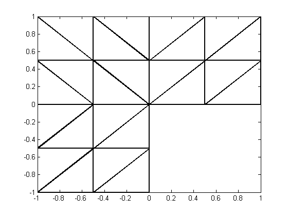
(a)

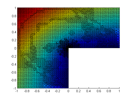
(b)

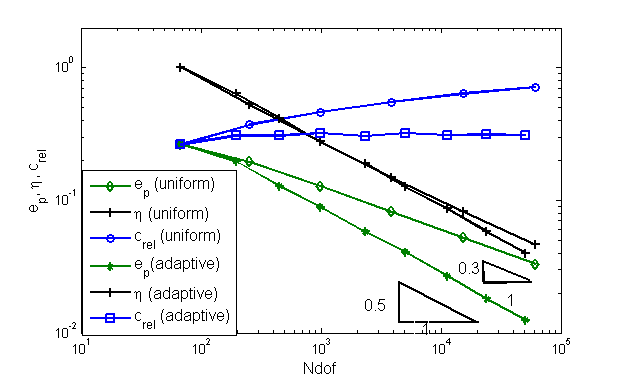
(c)

Figure 1: (a) Initial triangulation $\mathcal{T}_{0}$ (b) Discrete solution $u_{M}$ for adaptive mesh-refinement (c) Ndof vs. ${\bf e_{p}}$, $\eta$ and $C_{rel}$

Tables 1 and 2 show the errors and experimental convergence rate for uniform and adaptive mesh-refinements. Figure 1(a) denotes the initial triangulation $\mathcal{T}_{0}$ with $h\approx 0.5$. Figure 1(b) depicts the discrete solution $u_{M}$ and illustrates the adaptive mesh-refinement near the singularity. In Figure 1(c), a convergence history for the error ${\bf e_{p}}$ and the estimator $\eta$ is plotted as a function of the number of degrees of freedom for the cases of uniform and adaptive mesh-refinement of the non-convex L-shaped domain. Adaptive mesh refinement gives an optimal empirical convergence rate of order $0.5$ for ${\bf e_{p}}$, while standard uniform refinement achieves suboptimal empirical convergence rate $\approx 0.33$ as expected from the theory. For both the cases, $C_{rel}$, the ratio between the error and the estimator is also plotted.

Example 6.2

Crack problem: Consider the PDE (1.1) with coefficients $\mathbf{A}=I,~{}{\bf b}=(x-1,y+1)$ and $\gamma=0$ on$~{}\Omega=\{(x,y)\in\mathbb{R}^{2}:|{{\bf x}}|\leq 1\setminus[0,~{}1]\times\{0\}\}$ with Dirichlet boundary condition and exact solution $~{}u(r,\theta)=r^{{1}/{2}}\sin{\theta}/{2}-{r^{2}}/{2}\sin^{2}(\theta)$ ( in polar coordinates).

The problem is called non-coercive nochetto , since $(\gamma-\frac{1}{2}\nabla\cdot{\bf b})<0$. Figure 2(a) shows the discrete solution $u_{M}$ along with the adaptive mesh-refinement. Note that the mesh is strongly refined near the singularity at the origin. The results are summarized in Figure 2(b) and displays convergence rates for the error ${\bf e_{p}}$ and the a posteriori estimator $\eta$. It is observed that a suboptimal empirical convergence rate of $0.25$ for uniform mesh-refinement and an improved optimal empirical convergence rate of 0.5 for adaptive mesh-refinement are achieved. In this case, $C_{rel}$ is close to 0.5.

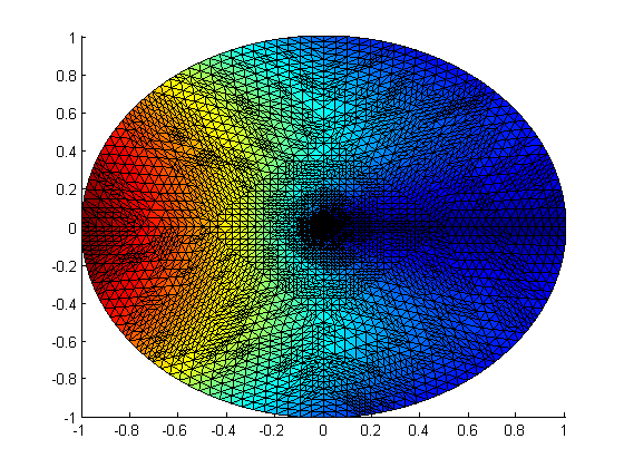
(a)

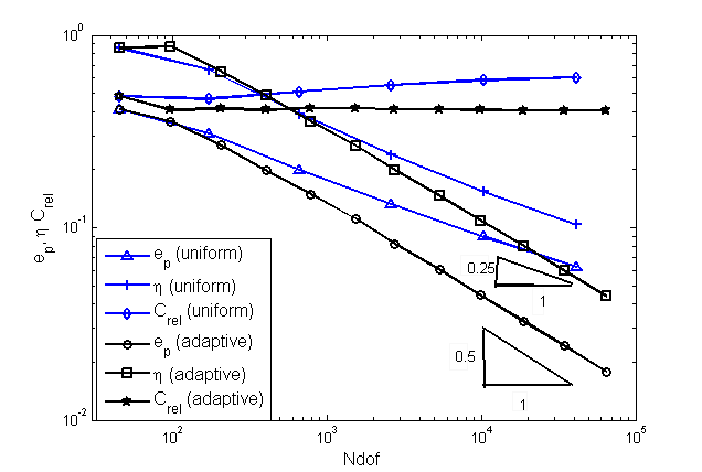
(b)

Figure 2: (a) Discrete solution $u_{M}$ for adaptive refinement (b) Ndof vs ${\bf e_{p}}$, $\eta$ and $C_{rel}$

Example 6.3

Consider the PDE (1.1) with coefficients $\mathbf{A}=I,~{}{\bf b}=(0,0)$ for different values of $\gamma$ and Dirichlet boundary conditions on the L-shaped domain.

Since the first Laplace eigenvalue for the L-shaped domain $\lambda_{1}\approx$ 9.6397238440219, the coefficients lead to the Laplace operator with positive and negative eigenvalues.

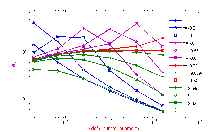
(a)

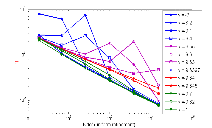
(b)

Figure 3: (a) $e_{p}$ and (b) $\eta$ for different $\gamma$ with uniform refinement

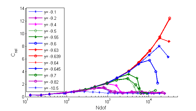
Figure 4: $C_{rel}$ for different $\gamma$ with adaptive refinement

The fact that the convergence is sensitive to the smallness of the discretization parameter $h$ is clearly observed in Figure 3(a). This observation holds true for conforming, nonconforming and mixed finite element methods. Figure 3(b) depicts that the estimator mirrors the error behavior.This is also true for the case of adaptive refinement.
Figure 4 plots the reliability constant $C_{rel}$ for various values of $\gamma$ close to the eigenvalue $\lambda_{1}$ vs the number of degrees of freedom. Note that $C_{rel}$ is sensitive to the discretization parameter $h$ especially when $\gamma$ is closer to $\lambda_{1}$. Thus, a sufficiently small mesh-size is a crucial requirement for the well-posedness and the convergence of the solution.

6.2 Conclusions

From the numerical experiments, it is observed that efficiency index lies between 2 and 3.5 for both uniform and adaptive triangulations. This confirms the efficiency of a posteriori error control for non-smooth problems defined in non-convex domains.
The overall assumption on the mesh-size to be sufficiently small is in fact crucial in practice, as shown in the third example empirically.

References

• (1) Arnold, D. N., Falk, R.S.: A uniformly accurate finite element method for the Reissner-Mindlin plate. SIAM J. Numer. Anal. 26, 1276-1290 (1989)
• (2) Bahriawati, C., Carstensen, C.: Three matlab implementations of the lowest order Raviart-Thomas MFEM with a posteriori error control. Comput. Methods Appl. Math. 5, 333-1361 (2005)
• (3) Brenner, S.C., Scott, L.R.: The mathematical theory of finite element methods. Springer, New York (2008)
• (4) Brenner, S.C.: Two-level additive Schwarz preconditioners for nonconforming finite element methods. Math. Comp. 65 , 897-921 (1996)
• (5) Brezzi, F., Fortin, M.: Mixed and hybrid finite element methods. Springer Verlag, New York (1991)
• (6) Carstensen, C.: A posteriori error estimate for the mixed finite element method. Math. Comp. 66, 465-476 (1997)
• (7) Carstensen, C.: A unifying theory of a posteriori finite element error control. Numer. Math. 100, 617-637 (2005)
• (8) Carstensen, C., Hu, J.: A unifying theory of a posteriori error control for nonconforming finite element methods. Numer. Math. 107, 473-502 (2007)
• (9) Carstensen, C., Eigel, M., Löbhard, C., Hoppe, R.H.W.: A review of unified a posteriori finite element error control. Numer. Math. Theory Methods Appl. 5, 509-558 (2012)
• (10) Chen, H., Xu, X., Hoppe, R. H. W.: Convergence and quasi-optimality of adaptive nonconforming finite element methods for some nonsymmetric and indefinite problems. Numer. Math. 116, 383-419 (2010)
• (11) Chen, J., Li, L.: Convergence and domain decomposition algorithm for nonconforming and mixed methods for nonselfadjoint and indefinite problems. Comput. Methods Appl. Mech. Engrg. 173, 1-20 (1999)
• (12) Ciarlet, P. Jr., Huang, J., Zou, J.: Some observations on generalized saddle-point problems. SIAM J Matrix Anal. Appl. 25, 224-236 (2003)
• (13) Douglas, J. Jr., Roberts, J. E.: Global estimates for mixed methods for second order elliptic equations. Math. Comp. 44, 39-52 (1985)
• (14) Douglas, J. Jr., Roberts, J. E.: Mixed finite element methods for second order elliptic problems. Mat. Apl. Comput. 1, 91-103 (1982)
• (15) Dauge, M.: Elliptic boundary problems on corner domains. Lecture Notes in Math. 1341, Springer-verlag, Berlin (1988)
• (16) Evans, L.C.: Partial Differential Equations. American Mathematical Society, Providence, Rhode Island (1998)
• (17) Gilberg, D., Trudinger, N.S.: Elliptic partial differential equations of second order. Springer-Verlag, Berlin (1983)
• (18) Mekchay, K., Nochetto,R.H.: Convergence of adaptive finite element methods for general second order linear elliptic PDEs. SIAM J. Numer. Anal. 43, 1803-1827 (2006)
• (19) Nicaise, S.: Polygonal interface problems. Verlag Peter D Lang, Frankfurt am Main (1993)
• (20) Schatz, A.H., Wang, J.: Some new error estimates for Ritz-Galerkin methods with minimal regularity assumptions. Math. Comp. 65, 19-27 (1996)
• (21) Verfürth, R: A review of a posteriori error estimation and adaptive mesh-refinement techniques. Wiley-Teubner, New York (1996)