Abstract

We calculate the next-to-leading-order QCD corrections to the perturbative term in the operator product expansion of the spectral functions of light tetraquark currents. By using also configuration-space methods we keep the momentum-space four-loop calculation to a manageable level. We find that the next-to-leading-order corrections to the perturbative term are large and can amount to $O(100\%)$. The corrections to the corresponding Borel sum rules, however, are small since the nonperturbative condensate contributions dominate the Borel sum rules.

PACS: 14.40.Rt, 12.38.Bx, 11.55.Hx

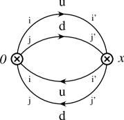
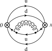
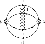
(a)(b)(c)

Figure 1: Leading-order tetraquark correlator (a) and two first-order corrections (b), (c)

1 Introduction

The nonet of light scalar mesons $\sigma(600)$, $\kappa(800)$, $a_{0}(980)$ and $f_{0}(980)$ are prime candidates for the long-sought-after light tetraquark states. Their mass ordering $m_{\sigma}<m_{\kappa}<m_{a_{0},f_{0}}$ precludes a simple $(\bar{q}q)$ interpretation [1, 2]. Also, in a $(\bar{q}q)$ picture, their masses are expected to lie above $1\mathop{\rm GeV}\nolimits$ contrary to experiment [3]. The spectrum of these four light scalar meson states fits perfectly into a picture where they are viewed as $L=0$ bound states of colour-, flavour- and spin-antisymmetric light diquarks and antidiquarks [1, 2]. In this picture one obtains a nonet of light scalar mesons composed of the states $a^{0}_{0}(I=1,I_{3}=0)/f_{0}(I=0)=([su][\bar{s}\bar{u}]\mp[sd][\bar{s}\bar{d}])/\sqrt{2}$, $\sigma(I=0)=[ud][\bar{u}\bar{d}]$, $\kappa^{0}=[ud][\bar{u}\bar{s}]$, $\bar{\kappa}^{0}=[us][\bar{u}\bar{d}]$ and the corresponding charged states $a^{\pm}_{0}$ and $\kappa^{\pm}$ in which the degeneracy of the two states $a^{0}_{0}$ and $f_{0}$ is natural and in which one obtains the above mass hierarchy $m_{\sigma}<m_{\kappa}<m_{a_{0},f_{0}}$ (see e.g. Refs. [4, 5]). Recently S. Weinberg has investigated tetraquarks in the large-$N_{c}$ limit of QCD [6] and found the existence of light tetraquark states to be consistent with large-$N_{c}$ QCD contrary to previous statements in the literature. An interesting development was described in Ref. [7]. Instantons produce an effective six-quark vertex which, among others, provides a mechanism for the decay $f_{0}(980)\to\pi\,\pi$.

A central theoretical issue is the need to theoretically understand the mass pattern of the light scalar states and whether a tetraquark interpretation of these states is able to accommodate or even predict the mass pattern of the light scalar states. This issue has been addressed in a number of recent theoretical investigations using the framework of QCD (Borel) sum rules to study the properties of light tetraquark states [8, 9, 10, 11, 12, 13, 14, 15, 16, 17, 18, 19]. Perhaps the most complete of these is the analysis by Chen, Hosaka and Zhu [11]. They studied the most general form of interpolating currents including possible mixing effects between them. In the operator product expansion they included up to dimension-eight operators. However, in their analysis and in previous analyses next-to-leading-order (NLO) QCD corrections to the leading-order (LO) perturbative term were not included. As has been emphasized by Zhang et al. one needs to calculate the $\alpha_{s}$ corrections to the current correlators in order to make the sum rule analysis reliable and predictable [20]. In momentum space ($p$ space) the NLO corrections to the light tetraquark current correlators or spectral functions require the calculation of massless four-loop diagrams which is not simple. However, if one also uses configuration space ($x$-space) techniques the task becomes simpler. This has been demonstrated in two previous papers where we have calculated the five-loop NLO corrections to pentaquark current correlators using also $x$-space techniques [21, 22]. The main idea of the $x$-space calculation is to first calculate two $x$-space modules corresponding to NLO propagator and dipropagator corrections and then to insert the modules into the full correlator diagram. In this way the calculation of radiative corrections to multiquark correlators amounts to purely algebraic manipulations.

The purpose of this paper is twofold. First we expound on the calculation of the two $O(\alpha_{s})$ modules that go into the modular approach to the calculation of radiative corrections to the current–current correlators of multiquark currents. As a new feature compared to [21, 22] we show, by using a general $R_{\xi}$ gauge, that the sum of the two modules is gauge invariant when sandwiched between colour-neutral states (mesons, baryons, tetraquarks and pentaquarks). Second, we present explicit results on the radiative corrections of light tetraquark current correlators for the two sets of five tetraquark currents (scalar, vector, tensor, axial vector and pseudoscalar, each for flavour-symmetric and -antisymmetric diquark configurations) that have been investigated in Refs. [9, 10, 11, 12]. We also present NLO results on all possible nondiagonal correlators.

Depending on the choice of tetraquark currents the radiative corrections to the LO perturbative term can amount to up to $132\%$ at $q^{2}=1\mathop{\rm GeV}\nolimits^{2}$ for the tensor current to be discussed later on. As a further exemplary case we consider the spectral density corresponding to the current correlator of a particular linear combination of the axial and vector tetraquark current $\eta_{1}^{\sigma}$ considered in Ref. [11]. The mixed current was found to be an optimal interpolating current with a good Borel window for the $\sigma$-meson tetraquark current [11]. For the corresponding spectral function we list the LO perturbative result and the NLO correction which is calculated in this paper. One has

$$\rho^{\sigma}_{1}(s)=\frac{s^{4}}{11520\pi^{6}}\bigg{\{}1+\frac{\alpha_{s}}{\pi}\bigg{(}\frac{7+6\sqrt{2}}{4}\ln\left(\frac{\mu_{\overline{\rm MS}}^{2}}{s}\right)+\frac{1381+15\sqrt{2}}{180}\bigg{)}\bigg{\}}$$ (1)

Using $\mu_{\overline{\rm MS}}^{2}=1\mathop{\rm GeV}\nolimits^{2}$ the NLO corrections can be seen to amount to a $55\%$ upward correction to the LO term at $q^{2}=1\mathop{\rm GeV}\nolimits^{2}$. Including also the nonperturbative contributions and using the central values for the masses and condensates from Ref. [11] one finds

$$\rho^{\sigma}_{1}(s=1\mathop{\rm GeV}\nolimits^{2})\ =\ \Big{(}9.03\,({\rm LO})+4.94\,({\rm NLO})$$ (2)

$$-0.042\,[d]^{2}+(83.89-5.80)\,[d]^{4}-0.045\,[d]^{6}-0.486\,[d]^{8}\Big{)}\cdot 10^{-8}\mathop{\rm GeV}\nolimits^{8}$$

The spectral function is dominated by the dimension-four gluon condensate contribution $\langle g^{2}GG\rangle$ listed as the first dimension-four term in Eq. (2). Such a large contribution does not appear to be very natural. We mention that the value of the gluon condensate has not yet been calculated from first principles but is obtained from fits to QCD sum rules. For example, the authors of Refs. [23, 24, 25] found $\langle g^{2}GG\rangle=(0.47\pm 0.47)\mathop{\rm GeV}\nolimits^{4}$ compared to $\langle g^{2}GG\rangle=(0.48\pm 0.14)\mathop{\rm GeV}\nolimits^{4}$ given in Ref. [26] and used by Chen et al. in Ref. [11]. This shows that a small or even vanishing contribution of the sum of the dimension-four condensates to the spectral function lies within a one-standard-deviation window of the central value if the results of Refs. [23, 24, 25] are used.

1.1 Interpolating currents

For the construction of interpolating currents we refer to the detailed presentation in Ref. [11]. Following these authors we obtain two sets of five currents each for the flavour-symmetric and -antisymmetric diquark–antidiquark states. For conciseness we specify our currents to the $(ud\bar{u}\bar{d})$ sector with hypercharge $Y=0$ which make up the $(ud\bar{u}\bar{d})$ components of the $\sigma,f_{0},a_{0}$ currents. In Ref. [11] one can find a detailed discussion about the flavour composition of the various tetraquark currents.

For the flavour-antisymmetric case one has the five currents

$$J_{S_{3}}^{\sigma} = (u^{iT}C\gamma_{5}d^{j})(\bar{u}_{i}\gamma_{5}C\bar{d}_{j}^{T}-\bar{u}_{j}\gamma_{5}C\bar{d}_{i}^{T}),$$

$$J_{V_{3}}^{\sigma} = (u^{iT}C\gamma^{\mu}\gamma_{5}d^{j})(\bar{u}_{i}\gamma_{\mu}\gamma_{5}C\bar{d}_{j}^{T}-\bar{u}_{j}\gamma_{\mu}\gamma_{5}C\bar{d}_{i}^{T}),$$

$$J_{T_{6}}^{\sigma} = (u^{iT}C\sigma^{\mu\nu}d^{j})(\bar{u}_{i}\sigma_{\mu\nu}C\bar{d}_{j}^{T}+\bar{u}_{j}\sigma_{\mu\nu}C\bar{d}_{i}^{T}),$$

$$J_{A_{6}}^{\sigma} = (u^{iT}C\gamma^{\mu}d^{j})(\bar{u}_{i}\gamma_{\mu}C\bar{d}_{j}^{T}+\bar{u}_{j}\gamma_{\mu}C\bar{d}_{i}^{T}),$$

$$J_{P_{3}}^{\sigma} = (u^{iT}Cd^{j})(\bar{u}_{i}C\bar{d}_{j}^{T}-\bar{u}_{j}C\bar{d}_{i}^{T}),$$ (3)

where $\sigma^{\mu\nu}=\frac{i}{2}[\gamma^{\mu},\gamma^{\nu}]$ (see also Appendix A). The lower index on the currents marks the colour multiplicity of the diquark state which is given by the antisymmetric (symmetric) colour representations in the decomposition ${\bf 3}\otimes{\bf 3}\Rightarrow{\bf\bar{3}_{a}}$ (${\bf 3}\otimes{\bf 3}\Rightarrow{\bf\bar{6}_{s}}$) and ${\bf\bar{3}}\otimes{\bf\bar{3}}\Rightarrow{\bf 3_{a}}$ (${\bf\bar{3}}\otimes{\bf\bar{3}}\Rightarrow{\bf\bar{6}_{s}}$). We mention that the mixed current correlator discussed above corresponds to the mixed current

$$J_{1}^{\sigma}=\cos\theta J_{A_{6}}^{\sigma}+\sin\theta J_{V_{3}}^{\sigma}$$ (4)

with $\tan\theta=\sqrt{2}$.

For the flavour-symmetric case one has the five currents

$$J_{S_{6}}^{\sigma} = (u^{iT}C\gamma_{5}d^{j})(\bar{u}_{i}\gamma_{5}C\bar{d}_{j}^{T}+\bar{u}_{j}\gamma_{5}C\bar{d}_{i}^{T}),$$

$$J_{V_{6}}^{\sigma} = (u^{iT}C\gamma^{\mu}\gamma_{5}d^{j})(\bar{u}_{i}\gamma_{\mu}\gamma_{5}C\bar{d}_{j}^{T}+\bar{u}_{j}\gamma_{\mu}\gamma_{5}C\bar{d}_{i}^{T}),$$

$$J_{T_{3}}^{\sigma} = (u^{iT}C\sigma^{\mu\nu}d^{j})(\bar{u}_{i}\sigma_{\mu\nu}C\bar{d}_{j}^{T}-\bar{u}_{j}\sigma_{\mu\nu}C\bar{d}_{i}^{T}),$$

$$J_{A_{3}}^{\sigma} = (u^{iT}C\gamma^{\mu}d^{j})(\bar{u}_{i}\gamma_{\mu}C\bar{d}_{j}^{T}-\bar{u}_{j}\gamma_{\mu}C\bar{d}_{i}^{T}),$$

$$J_{P_{6}}^{\sigma} = (u^{iT}Cd^{j})(\bar{u}_{i}C\bar{d}_{j}^{T}+\bar{u}_{j}C\bar{d}_{i}^{T}).$$ (5)

Except for the LO term the $O(\alpha_{s})$ perturbative contributions to the flavour-symmetric and -antisymmetric correlators are not always simply related. The currents in Eqs. (1.1) and (1.1) are built from diquark–antidiquark components. One can also construct the tetraquark currents from meson–meson components. However, the meson–meson currents do not lead to new tetraquark configurations since the two representations are related by a Fierz transformation (see Ref. [11] and Appendix B).

For an understanding and illustration of the modular approach it is sufficient to discuss a simplified form of the scalar current given by

$$J_{S}(x) = \left(u^{iT}(x)C\gamma_{5}d^{j}(x)\right)\left(\bar{u}_{i}(x)\gamma_{5}C\bar{d}_{j}^{T}(x)\right)$$ (6)

$$= \delta_{i}^{k}\delta_{j}^{l}\left(u^{iT}(x)C\gamma_{5}d^{j}(x)\right)\left(\bar{u}_{k}(x)\gamma_{5}C\bar{d}_{l}^{T}(x)\right),$$

involving only the first part of the scalar current in Eq. (1.1). It is not difficult to reinstate the colour-symmetrized/-antisymmetrized form of the current at the final stages of the calculations.

1.2 The correlator

The correlation function is defined as the vacuum expectation value of the time-ordered product of two currents, i.e.

$$\Pi(x)=\langle 0|\mathcal{T}\{J(x)\bar{J}(0)\}|0\rangle.$$ (7)

If the current describes a boson (meson or tetraquark), one has $\bar{J}(0)=J^{\dagger}(0)$ while in case of a fermion (baryon or pentaquark), one has $\bar{J}(0)=J^{\dagger}(0)\gamma^{0}$.

The correlator in Eq. (7) is defined in $x$ space. It can be transformed to $p$ space by a Fourier transformation with the result

$$\Pi(q)=i\int\Pi(x)e^{iqx}d^{4}x=i\int\langle 0|\mathcal{T}\{J(x)\bar{J}(0)\}|0\rangle e^{iqx}d^{4}x,$$ (8)

where, for the moment, we work in $D=4$ dimensions. The optical theorem relates the $p$-space correlator to the spectral density

$$\rho(s)=\frac{1}{2\pi i}\mathop{\rm Disc}\nolimits\Pi(q)|_{q^{2}=-s},$$ (9)

where the discontinuity $\mathop{\rm Disc}\nolimits f(p)$ is defined by (see e.g. Ref. [27])

$$\mathop{\rm Disc}\nolimits f(p):=f(pe^{i0})-f(pe^{-i0}),\qquad e^{\pm i0}=\lim_{\varepsilon\to 0}e^{\pm i\varepsilon},\ \varepsilon>0.$$ (10)

Vice versa, for a given spectral density, the correlator can be reconstructed by using

$$\Pi(q)=\int_{0}^{\infty}\frac{\rho(s)ds}{s+q^{2}}.$$ (11)

For the simplified scalar current in Eq. (6) the tetraquark correlator in $x$ space reads

$$\Pi(x)=\mathop{\rm Tr}\nolimits\Big{(}S_{u}(x)^{i}_{i^{\prime}}\gamma_{5}S_{d}(x)^{j}_{j^{\prime}}\gamma_{5}\Big{)}\mathop{\rm Tr}\nolimits\Big{(}S_{u}(-x)^{i^{\prime}}_{i}\gamma_{5}S_{d}(-x)^{j^{\prime}}_{j}\gamma_{5}\Big{)}=\frac{9}{\pi^{8}x^{12}}$$ (12)

where we have made use of the $x$-space propagator given by $S(x)^{i}_{i^{\prime}}=\delta^{i}_{i^{\prime}}S_{0}(-x^{2})x^{\mu}\gamma_{\mu}$ with $S_{0}(x^{2})=(2\pi^{2}x^{4})^{-1}$ for $D=4$ (cf. Eq. (14)). The first trace in Eq. (12) contains two quark propagators with a positive $x$-space argument while the second trace contains two antiquark propagators corresponding to quark propagators with a negative $x$-space argument. The general rule is that an antiquark propagator carries an extra minus sign. Note that the colour trace in Eq. (12) connects quarks/antiquarks in the two different Dirac traces.

2 Propagator and dipropagator modules

The result in Eq. (12) reflects a very general property of massless correlators represented by sunrise-type diagrams: in $x$ space they are obtained by a product of single $x$-space propagators. The corresponding $p$-space calculation is far more difficult since one would have to perform a genuine three-loop calculation. This observation sets the strategy for the evaluation of the radiative corrections to the tetraquark correlator: do most of the calculation in $x$ space. In detail, we first calculate the radiative corrections to a single propagator and the dipropagator in $p$ space (see Fig. 2). We shall refer to these two corrections as the propagator and dipropagator modules. In the two modules the Dirac and colour indices are left open. We then Fourier transform the two modules to $x$ space. Next we assemble the $x$-space tetraquark correlator from these two modules augmented by free propagators as shown in in Fig. 2. The assembly is simple in $x$ space since the free propagators are linked to the modules in product form. One then does the appropriate Dirac and colour contractions according to the specific current being investigated. Finally, we Fourier transform the $x$-space tetraquark correlator back to $p$ space.

In the following section we first calculate the $p$-space propagator and the dipropagator corrections using traditional momentum integration methods. The propagator and the dipropagator corrections are then transformed to $x$ space.

2.1 The propagator correction

For illustrative reasons we begin by considering the LO massless propagator in $p$ space which takes the familiar form

$$S_{1}^{0}(q)=\frac{i}{q\kern-5.5pt/}=-iq_{\mu}\gamma^{\mu}(-q^{2})^{-1}.$$ (13)

In order to obtain the corresponding LO $x$-space propagator we have to take the Fourier transform of the propagator in Eq. (13). Since we are working in dimensional regularization one needs to make use of the $D$-dimensional Fourier transform ($D=4-2\varepsilon$). The relevant $D$-dimensional transformation formulas are collected in Appendix C. One obtains

$$S_{1}^{0}(x)=S_{0}(-x^{2})x_{\mu}\gamma^{\mu},$$ (14)

where we have factored out a frequently occurring function $S_{0}(-x^{2})$ defined by

$$S_{0}(-x^{2})=\frac{\Gamma(2-\varepsilon)}{2(4\pi)^{2-\varepsilon}}\left(-\frac{x^{2}}{4}\right)^{\varepsilon-2}=\frac{\Gamma(2-\varepsilon)}{2\pi^{2-\varepsilon}(-x^{2})^{2-\varepsilon}}.$$ (15)

In Feynman gauge and in $p$ space the propagator correction (see Fig. 2(a)) reads

$$S_{1}^{1}(q)=\frac{i}{q\kern-5.5pt/}\int\frac{d^{D}k}{(2\pi)^{D}}(-i\tilde{g}_{s}\gamma^{\alpha}T_{a})\frac{i}{/\kern-6.0ptk}(-i\tilde{g}_{s}\gamma^{\beta}T_{b})\frac{i}{q\kern-5.5pt/}\,\frac{-ig_{\alpha\beta}\delta_{ab}}{(q-k)^{2}}.$$ (16)

In Eqs. (13)–(16) we have suppressed the colour index dependence $\delta_{i}^{j}$.

Let us briefly comment on the gauge dependence of our results. In a general $R_{\xi}$ gauge the gluon propagator reads

$$D_{\alpha\beta}(k)=\frac{i}{k^{2}}\left(-g_{\alpha\beta}+(1-\xi)\frac{k_{\alpha}k_{\beta}}{k^{2}}\right).$$ (17)

The Feynman gauge used in Eq. (16) corresponds to the choice $\xi=1$. As shown in Appendix D, the gauge dependence drops out in the sum of the propagator and dipropagator corrections when sandwiched between colour-neutral states.

Returning to Eq. (16) we proceed with the Feynman gauge calculation and obtain

$$S_{1}^{1}(q) = (D-2)\tilde{g}_{s}^{2}T_{a}T_{a}\frac{i}{q\kern-5.5pt/}\int\frac{d^{D}k}{(2\pi)^{D}}\frac{/\kern-6.0ptk}{k^{2}(q-k)^{2}}\frac{i}{q\kern-5.5pt/}.$$ (18)

It is convenient to define the dimensionless one-loop two-point integrals $G(n_{1},n_{2})$ through

$$\frac{i}{(4\pi)^{D/2}}(-q^{2})^{D/2-n_{1}-n_{2}}G(n_{1},n_{2}):=\int\frac{d^{D}k}{(2\pi)^{D}}\frac{1}{(-k^{2})^{n_{1}}(-(q-k)^{2})^{n_{2}}}.$$ (19)

After setting the tadpole contributions to zero, the integral in Eq. (18) can be expressed in terms of the standard integral $G(1,1)$ given by

$$G(1,1)=\frac{\Gamma(\varepsilon)\Gamma^{2}(1-\varepsilon)}{\Gamma(2-2\varepsilon)}=\frac{\Gamma(1+\varepsilon)\Gamma^{2}(1-\varepsilon)}{\varepsilon\Gamma(2-2\varepsilon)}=:\frac{G}{\varepsilon}.$$ (20)

The one-loop integral $G(1,1)$ is divergent. In Eq. (20) we have introduced the factor $G=\Gamma(1+\varepsilon)\Gamma^{2}(1-\varepsilon)/\varepsilon\Gamma(2-2\varepsilon)$ because we want to absorb the $\Gamma$ factors in Eq. (20) into the definition of the renormalization scale. We shall refer to this scheme as the $G$ scheme. The relation to the (modified) minimal substraction scheme is given by

$$\mu_{G}^{2\varepsilon}=G(4\pi\mu_{\rm MS}^{2})^{\varepsilon},\qquad\mu_{G}^{2}\approx e^{2}\mu_{\overline{\rm MS}}^{2}=4\pi e^{2-\gamma_{E}}\mu_{\rm MS}^{2}.$$ (21)

The corrected NLO $p$-space propagator finally reads

$$S_{1}^{1}(q)=-\frac{\alpha_{s}C_{F}}{4\pi}\left(\frac{1}{\varepsilon}-1\right)\left(-\frac{q^{2}}{\mu_{G}^{2}}\right)^{-\varepsilon}\frac{i}{q\kern-5.5pt/}.$$ (22)

With the help of Eq. (C7) in Appendix C (with $\alpha=1+\varepsilon$) one obtains the corresponding $x$-space result

$$S_{1}^{1}(x)=-S_{0}(-x^{2})\frac{\alpha_{s}C_{F}}{4\pi}\left(\frac{1}{\varepsilon}+O(\varepsilon)\right)(-\mu_{x}^{2}x^{2})^{\varepsilon}x_{\mu}\gamma^{\mu}.$$ (23)

We have introduced an $x$-space scale $\mu_{x}$ as a new renormalization scale, defined by

$$\mu_{x}^{2\varepsilon}=\frac{\Gamma(1-\varepsilon)}{(4\pi)^{-\varepsilon}}\left(\frac{1}{4}\right)^{\varepsilon}\mu_{\rm MS}^{2\varepsilon},\qquad 4\mu_{x}^{2}=4\pi e^{\gamma_{E}}\mu_{\rm MS}^{2}+O(\varepsilon)=e^{2\gamma_{E}}\mu_{\overline{\rm MS}}^{2}+O(\varepsilon).$$ (24)

Altogether the $O(\alpha_{s})$ $x$-space propagator reads

$$S_{1}(x)=S_{0}(-x^{2})\left\{1-\frac{\alpha_{s}C_{F}}{4\pi}\left(\frac{1}{\varepsilon}+O(\varepsilon)\right)(-\mu_{x}^{2}x^{2})^{\varepsilon}+O(\alpha_{s}^{2})\right\}x_{\mu}\gamma^{\mu}.$$ (25)

As expected, the propagator correction has the spatial structure of the LO term in Eq. (14).

(a)(b)

Figure 2: Propagator correction (a) with loop momentum $k$ and dipropagator correction (b) with loop momenta $l$ and $k$

2.2 The dipropagator correction

In order to familiarize the reader with the calculational procedure and the notation, we start our discussion with the calculation of the uncorrected dipropagator. In $p$ space the uncorrected dipropagator consists of a single loop integral where the two pairs of Dirac and colour indices are left open and uncontracted. The one-loop integral reads (colour indices are suppressed)

$$S_{2}^{0}(q)=\int\frac{d^{D}k}{(2\pi)^{D}}\left(\frac{i}{/\kern-6.0ptk}\otimes\frac{i}{q\kern-5.5pt/-/\kern-6.0ptk}\right)=\int\frac{d^{D}k}{(2\pi)^{D}}\frac{k_{\mu}(q-k)_{\nu}}{k^{2}(q-k)^{2}}(\gamma^{\mu}\otimes\gamma^{\nu})=I_{\mu\nu}^{0}(q)(\gamma^{\mu}\otimes\gamma^{\nu}).$$ (26)

Expanding the tensor integral $I_{\mu\nu}^{0}$ into the two covariants $q^{2}g_{\mu\nu}$ and $q_{\mu}q_{\nu}$, one has

$$I_{\mu\nu}^{0}(q)=\int\frac{d^{D}k}{(2\pi)^{D}}\frac{k_{\mu}(q-k)_{\nu}}{k^{2}(q-k)^{2}}=A^{0}q_{\mu}q_{\nu}+B^{0}q^{2}g_{\mu\nu}.$$ (27)

By contracting Eq. (27) with $g^{\mu\nu}$ and $q^{\mu}q^{\nu}$, calculating the resulting scalar integrals, dropping tadpole contributions and solving for $A^{0}$ and $B^{0}$ one obtains

$$A^{0}=\frac{-iG(1,1)(D-2)}{4(4\pi)^{D/2}(D-1)}(-q^{2})^{D/2-2},\qquad B^{0}=\frac{-iG(1,1)}{4(4\pi)^{D/2}(D-1)}(-q^{2})^{D/2-2},$$ (28)

where the scalar integral $G(1,1)$ is listed in Eq. (20). Altogether one has

$$S_{2}^{0}(q)=\frac{-iG(1,1)}{4(4\pi)^{D/2}(D-1)}(-q^{2})^{D/2-2}\Big{(}(D-2)q_{\mu}q_{\nu}+q^{2}g_{\mu\nu}\Big{)}(\gamma^{\mu}\otimes\gamma^{\nu}).$$ (29)

We then Fourier transform $S_{2}^{0}(q)$ to $x$ space using the results in Appendix C (Eq. (C9) with $\alpha=2-D/2=\varepsilon$, $A=D-2=2(1-\varepsilon)$ and $B=1$). One obtains

$$S_{2}^{0}(x) = \frac{G(1,1)\Gamma(D-1)}{32(4\pi)^{D}(D-1)\Gamma(2-D/2)}\left(-\frac{x^{2}}{4}\right)^{-D}\Big{(}-2(D-1)(D-2)x_{\mu}x_{\nu}\Big{)}(\gamma^{\mu}\otimes\gamma^{\nu})$$ (30)

$$= (S_{0}(-x^{2}))^{2}x_{\mu}x_{\nu}(\gamma^{\mu}\otimes\gamma^{\nu})\ =\ S_{1}^{0}(x)\otimes S_{1}^{0}(x).$$

where $S_{1}^{0}(x)$ is defined in Eq. (14). The factorized result in the second line of Eq. (30) is a special case of the general $x$-space result for a massless $n$-loop sunrise diagram written down in Refs. [27, 28, 29, 30].

In order to calculate the NLO dipropagator correction we start again in $p$ space. A symbolic representation of the corresponding two-loop Feynman diagram is shown in Fig. 2(b). The endpoints of the momentum lines in the initial and final states have not been joined together in order to symbolize the fact that the colour and Dirac indices in the diagram are left open. The two-loop correction to the dipropagator is given by the twofold integral

$$S_{2}^{1}(q) = \int\frac{d^{D}k}{(2\pi)^{D}}\frac{d^{D}l}{(2\pi)^{D}}\left(\frac{i}{/\kern-6.0ptk}(-i\tilde{g}_{s}\gamma^{\alpha}T_{a})\frac{i}{/\kern-4.0ptl}\otimes\frac{i}{q\kern-5.5pt/-/\kern-6.0ptk}(-i\tilde{g}_{s}\gamma^{\beta}T_{b})\frac{i}{q\kern-5.5pt/-/\kern-4.0ptl}\right)\frac{-ig_{\alpha\beta}\delta_{ab}}{(k-l)^{2}}$$ (31)

$$= (T_{a}\otimes T_{a})\tilde{g}_{s}^{2}(\gamma^{\mu}\gamma^{\alpha}\gamma^{\nu}\otimes\gamma_{\mu^{\prime}}\gamma_{\alpha}\gamma_{\nu^{\prime}})I^{\mu^{\prime}\nu^{\prime}}_{\mu\nu}(q),$$

where

$$I^{\mu^{\prime}\nu^{\prime}}_{\mu\nu}(q)=i\int\frac{d^{D}k}{(2\pi)^{D}}\frac{d^{D}l}{(2\pi)^{D}}\frac{k_{\mu}l_{\nu}(q-k)^{\mu^{\prime}}(q-l)^{\nu^{\prime}}}{k^{2}l^{2}(q-k)^{2}(q-l)^{2}(k-l)^{2}}.$$ (32)

The integral $I^{\mu^{\prime}\nu^{\prime}}_{\mu\nu}(q)$ can be seen to be symmetric under the simultaneous interchange of $\mu\leftrightarrow\nu$ and $\mu^{\prime}\leftrightarrow\nu^{\prime}$. It is therefore expedient to split the gamma matrix string $\gamma^{\mu}\gamma^{\alpha}\gamma^{\nu}$ (and, accordingly, $\gamma_{\mu^{\prime}}\gamma_{\alpha}\gamma_{\nu^{\prime}}$) into its $\mu\leftrightarrow\nu$ and $\mu^{\prime}\leftrightarrow\nu^{\prime}$ symmetric and antisymmetric parts,

$$\gamma^{\mu}\gamma^{\alpha}\gamma^{\nu}=\frac{1}{2}(\gamma^{\mu}\gamma^{\alpha}\gamma^{\nu}+\gamma^{\nu}\gamma^{\alpha}\gamma^{\mu})+\frac{1}{2}(\gamma^{\mu}\gamma^{\alpha}\gamma^{\nu}-\gamma^{\nu}\gamma^{\alpha}\gamma^{\mu})=\gamma^{(\mu}\gamma^{\alpha}\gamma^{\nu)}+\gamma^{[\mu}\gamma^{\alpha}\gamma^{\nu]}.$$ (33)

One then remains with

$$(\gamma^{\mu}\gamma^{\alpha}\gamma^{\nu}\otimes\gamma_{\mu^{\prime}}\gamma_{\alpha}\gamma_{\nu^{\prime}})I^{\mu^{\prime}\nu^{\prime}}_{\mu\nu}(q)\ =$$ (34)

$$= (\gamma^{(\mu}\gamma^{\alpha}\gamma^{\nu)}\otimes\gamma_{(\mu^{\prime}}\gamma_{\alpha}\gamma_{\nu^{\prime})})I^{(\mu^{\prime}\nu^{\prime})}_{(\mu\nu)}(q)+(\gamma^{[\mu}\gamma^{\alpha}\gamma^{\nu]}\otimes\gamma_{[\mu^{\prime}}\gamma_{\alpha}\gamma_{\nu^{\prime}]})I^{[\mu^{\prime}\nu^{\prime}]}_{[\mu\nu]}(q).\qquad$$

The symmetric–symmetric contribution in Eq. (34) will be dealt with by making use of the $D$-dimensional identity $\gamma^{(\mu}\gamma^{\alpha}\gamma^{\nu)}=(g^{\mu\alpha}g^{\nu\beta}+g^{\mu\beta}g^{\nu\alpha}-g^{\mu\nu}g^{\alpha\beta})\gamma_{\beta}$ and the corresponding identity for $\gamma_{(\mu^{\prime}}\gamma_{\alpha}\gamma_{\nu^{\prime})}$.

The contraction $(\gamma^{(\mu}\gamma^{\alpha}\gamma^{\nu)}\otimes\gamma_{(\mu^{\prime}}\gamma_{\alpha}\gamma_{\nu^{\prime})})\,I^{(\mu^{\prime}\nu^{\prime})}_{(\mu\nu)}(q)$ leads to a number of second-rank two-loop tensor integrals which can be reduced to scalar integrals using standard techniques. In order to minimize calculational mistakes, all necessary manipulations have been done by computer algebra programs. The required set of scalar two-loop integrals needed in this application are defined by [33]

$$\frac{-1}{(4\pi)^{D}}(-q^{2})^{D-n_{1}-n_{2}-n_{3}-n_{4}-n_{5}}G(n_{1},n_{2},n_{3},n_{4},n_{5})\ :=$$ (35)

$$= \int\frac{d^{D}k}{(2\pi)^{D}}\frac{d^{D}l}{(2\pi)^{D}}\frac{1}{(-k^{2})^{n_{1}}(-l^{2})^{n_{2}}(-(q-k)^{2})^{n_{3}}(-(q-l)^{2})^{n_{4}}(-(k-l)^{2})^{n_{5}}}.\qquad$$

Their solution has been given in Ref. [33].

The symmetric–symmetric contribution to the dipropagator correction can be represented in the form

$$S_{2}^{S1}(q)=(T_{a}\otimes T_{a})(I_{S})_{\beta}{}^{\beta^{\prime}}(q)(\gamma^{\beta}\otimes\gamma_{\beta^{\prime}}),$$ (36)

where

$$(I_{S})_{\beta}{}^{\beta^{\prime}}(q)=A_{1}(q^{2})q_{\beta}q^{\beta^{\prime}}+B_{1}(q^{2})q^{2}g_{\beta}^{\beta^{\prime}},$$ (37)

and where

$$A_{1}(q^{2})=\frac{i\tilde{g}_{s}^{2}G^{2}(-q^{2})^{-2\varepsilon}}{(4\pi)^{4-2\varepsilon}\varepsilon^{2}}\left(\frac{1-5\varepsilon}{12}\right),\qquad B_{1}(q^{2})=\frac{i\tilde{g}_{s}^{2}G^{2}(-q^{2})^{-2\varepsilon}}{(4\pi)^{4-2\varepsilon}\varepsilon^{2}}\left(\frac{7+13\varepsilon}{24}\right).$$ (38)

Next we turn to the antisymmetric–antisymmetric contribution in Eq. (34) whose structure can be further specified by noting that the integral $I_{[\mu\nu]}^{[\mu^{\prime}\nu^{\prime}]}(q)$ is separately antisymmetric under the exchange $\mu\leftrightarrow\nu$ and $\mu^{\prime}\leftrightarrow\nu^{\prime}$. The integral $I_{[\mu\nu]}^{[\mu^{\prime}\nu^{\prime}]}(q)$ can thus be expanded into two corresponding tensors built from the metric tensor and the outer momentum $q$ that possess this antisymmetry. One therefore has

$$I_{[\mu\nu]}^{[\mu^{\prime}\nu^{\prime}]}(q)=\Big{(}q_{\mu}(g_{\nu}^{\nu^{\prime}}q^{\mu^{\prime}}-g_{\nu}^{\mu^{\prime}}q^{\nu^{\prime}})+q_{\nu}(g_{\mu}^{\mu^{\prime}}q^{\nu^{\prime}}-g_{\mu}^{\nu^{{}^{\prime}}}q^{\mu^{\prime}})\Big{)}R_{1}+(g_{\mu}^{\mu^{\prime}}g_{\nu}^{\nu^{\prime}}-g_{\mu}^{\nu^{\prime}}g_{\nu}^{\mu^{\prime}})R_{2}.$$ (39)

Using again standard techniques one obtains the contributions of the antisymmetric–antisymmetric part in terms of a set of fourth-order tensor integrals which can again be reduced to the two-loop scalar integrals in Eq. (35).

Similar to Eq. (36) the antisymmetric–antisymmetric contribution to the dipropagator correction can be written in the form

$$S_{2}^{A1}(q)=(T_{a}\otimes T_{a})(I_{A})_{\beta}{}^{\beta^{\prime}}(q)(\gamma^{[\mu}\gamma^{\beta}\gamma^{\nu]}\otimes\gamma_{[\mu^{\prime}}\gamma_{\beta^{\prime}}\gamma_{\nu^{\prime}]})$$ (40)

with

$$(I_{A})_{\beta}{}^{\beta^{\prime}}(q)=A_{3}(q^{2})q_{\beta}q^{\beta^{\prime}}+B_{3}(q^{2})q^{2}g_{\beta}^{\beta^{\prime}},$$ (41)

and

$$A_{3}(q^{2})=\frac{i\tilde{g}_{s}^{2}G^{2}(-q^{2})^{-2\varepsilon}}{(4\pi)^{4-2\varepsilon}\varepsilon^{2}}\left(\frac{1}{24}\right),\qquad B_{3}(q^{2})=\frac{i\tilde{g}_{s}^{2}G^{2}(-q^{2})^{-2\varepsilon}}{(4\pi)^{4-2\varepsilon}\varepsilon^{2}}\left(\frac{1+2\varepsilon}{48}\right).$$ (42)

Adding up the symmetric–symmetric contribution in Eq. (36) and the antisymmetric–antisymmetric contribution in Eq. (40) the final result in $p$ space reads

$$S_{2}^{1}(q) = (T_{a}\otimes T_{a})\frac{i\tilde{g}_{s}^{2}G^{2}(-q^{2})^{-2\varepsilon}}{(4\pi)^{4-2\varepsilon}\varepsilon^{2}}\Big{\{}(a_{1}q_{\beta}q^{\beta^{\prime}}+b_{1}q^{2}g_{\beta}^{\beta^{\prime}})(\gamma^{\beta}\otimes\gamma_{\beta^{\prime}})$$ (43)

$$+(a_{3}q_{\beta}q^{\beta^{\prime}}+b_{3}q^{2}g_{\beta}^{\beta^{\prime}})(\gamma^{[\mu}\gamma^{\alpha}\gamma^{\beta]}\otimes\gamma_{[\mu}\gamma_{\alpha}\gamma_{\beta^{\prime}]})\Big{\}},$$

where

$$a_{1}=\frac{1}{12}(1-5\varepsilon),\qquad b_{1}=\frac{1}{24}(7+13\varepsilon),\qquad a_{3}=\frac{1}{24},\qquad b_{3x}=\frac{1}{48}(1+2\varepsilon).$$ (44)

The result is then Fourier transformed to $x$ space using again the results of Appendix C. Together with the LO result one finally has $S_{2}(x)=S_{2}^{0}(x)+S_{2}^{1}(x)$,

$$S_{2}(x) = (S_{0}(-x^{2}))^{2}\bigg{\{}\bigg{[}\bigg{(}1-(T_{a}\otimes T_{a})\frac{\alpha_{s}}{4\pi}(-\mu_{x}^{2}x^{2})^{\varepsilon}\left(\frac{1}{\varepsilon}+\frac{11}{2}\right)x_{\mu}x_{\nu}$$ (45)

$$-(T_{a}\otimes T_{a})\frac{\alpha_{s}}{4\pi}(-\mu_{x}^{2}x^{2})^{\varepsilon}\left(\frac{1}{\varepsilon}+\frac{1}{2}\right)x^{2}g_{\mu\nu}\bigg{]}(\gamma^{\mu}\otimes\gamma^{\nu})$$

$$-(T_{a}\otimes T_{a})\frac{\alpha_{s}}{4\pi}(-\mu_{x}^{2}x^{2})^{\varepsilon}\left(\frac{1}{2\varepsilon}+\frac{1}{4}\right)x_{\mu}x_{\nu}(\gamma^{[\alpha}\gamma^{\beta}\gamma^{\mu]}\otimes\gamma_{[\alpha}\gamma_{\beta}\gamma^{\nu]})\bigg{\}}.\qquad$$

It is important to realize that the dipropagator module contains terms which do not have the spatial structure of the LO term in Eq. (43).

3 Renormalization

In as much as the divergence of the propagator can be removed by renormalizing the wave function, one can remove the divergences of the correlator $\Pi$ by renormalizing the currents $J$. There is an important difference, though, in as much as the corrected correlator may contain higher-order spinor field products that differ from the LO currents. Therefore, we must take into account both multiplicative renormalization and additive counterterms. If $J^{(0)}(x)$ is the LO current and $\Delta J^{(1)}(x)$ is the first-order correction, the first-order correction of the correlator in Eq. (7) is given by

$$\Delta\Pi^{(1)}(x)=\langle 0|\mathcal{T}\{J^{(0)}(x)\Delta\bar{J}^{(1)}(0)+\Delta J^{(1)}(x)\bar{J}^{(0)}(0)\}|0\rangle.$$ (46)

3.1 Renormalization factor

The wave-function renormalization is calculated by using the propagator correction. The wave-function renormalization is always multiplicative since the propagator correction does not change the structure of the current. The renormalization factor is a perturbation series in the corresponding subtraction scheme which consists of pure poles to every order. The renormalization factor for the propagator correction (25) reads

$$Z_{2}=1+\sum_{n=1}^{\infty}\left(\frac{\alpha_{s}}{4\pi}\right)^{n}\sum_{m=1}^{n}\frac{1}{\varepsilon^{m}}Z_{n}^{m}=1+\frac{\alpha_{s}}{4\pi\varepsilon}Z_{1}^{1}+O(\alpha_{s}^{2})$$ (47)

with the condition that $Z_{2}^{-1}S_{1}(x)=:S_{1}^{r}(x)$ is finite. As a result we obtain the renormalization factor

$$Z_{2}=1-\frac{\alpha_{s}C_{F}}{4\pi\varepsilon}=1-\frac{\alpha_{s}}{3\pi\varepsilon}.$$ (48)

Therefore, we renormalize the singularity of the propagator corrections by multiplying the correlator with $Z_{2}^{-n}$, where $n$ is the number of lines ($n=4$ for the tetraquark).

3.2 Counterterms

The first-order QCD dipropagator correction changes the quark spinor fields $q(x)$. In $x$ space the change due to gluon exchange is given by

$$\Delta q(x)=-ig_{s}\int d^{D}x^{\prime}S(x-x^{\prime})\gamma^{\mu}T_{a}q(x^{\prime})A_{\mu}^{a}(x^{\prime}).$$ (49)

where $A_{\mu}^{a}(x^{\prime})$ is the gluon field. In the case of the tetraquark current one has four different species of spinor fields: $q(x)$, $\bar{q}(x)$, $q^{T}(x)C$, and $C\bar{q}^{T}(x)$. The corresponding changes under gluon exchange for the current at $x=0$ (the current at $x\neq 0$ is dealt with accordingly) are given by

$$\Delta q_{i} = -ig_{s}(T_{a})_{ii^{\prime}}\int d^{4}x\,S_{\alpha}(-x)A_{\beta}^{a}(x)\gamma^{\alpha}\gamma^{\beta}q_{i^{\prime}}(x),$$

$$\Delta\bar{q}_{i} = -ig_{s}\int d^{4}x\,\bar{q}_{i^{\prime}}(x)\gamma^{\beta}\gamma^{\alpha}S_{\alpha}(x)A_{\beta}^{a}(x)(T_{a})_{i^{\prime}i},$$

$$\Delta q_{i}^{T}C = -ig_{s}(T_{a})_{ii^{\prime}}\int d^{4}x\,q_{i^{\prime}}^{T}(x)C\gamma^{\beta}\gamma^{\alpha}S_{\alpha}(x)A_{\beta}^{a}(x),$$

$$C\Delta\bar{q}_{i}^{T} = -ig_{s}\int d^{4}x\,A_{\beta}^{a}(x)S_{\alpha}(-x)\gamma^{\alpha}\gamma^{\beta}C\bar{q}_{i^{\prime}}^{T}(x)(T_{a})_{i^{\prime}i}.$$ (50)

In the dipropagator correction the gluon fields of two spinor corrections have to be linked to build a gluon propagator. Therefore, one has to calculate

$$-g_{s}^{2}\int d^{D}x^{\prime}d^{D}x^{\prime\prime}S_{\alpha}(s_{1}x^{\prime})D_{\mu\nu}(x^{\prime}-x^{\prime\prime})S_{\beta}(s_{2}x^{\prime\prime})\ =$$ (51)

$$= is_{1}s_{2}g_{s}^{2}\int\frac{d^{D}k}{(2\pi)^{D}}\frac{k_{\alpha}k_{\beta}}{(k^{2}-m_{G}^{2})^{3}}g_{\mu\nu}\ =\ \frac{-s_{1}s_{2}\alpha_{s}}{16\pi\varepsilon}g_{\alpha\beta}g_{\mu\nu}+\mbox{finite terms},$$

where $s_{1}$ and $s_{2}$ are the signs of the two propagator arguments. Note that we can perform the integration over $x^{\prime}$ and $x^{\prime\prime}$ because we are looking for the UV-singular part. In $x$ space, the UV regime means locality, i.e. one can replace $\psi(x^{\prime})$ and $\psi(x^{\prime\prime})$ under the integrations by $\psi(x)$. In addition, we have used a (small) gluon mass $m_{G}$ in order to regularize IR singularities. We have kept only the UV-singular terms because in order to calculate the counterterm we stay in the same renormalization scheme, i.e. we do not subtract finite terms. Taking these considerations into account, the changes for the different formal products of two spinors read

$$\Delta(q^{i}\otimes q^{j}) = \frac{-\alpha_{s}}{16\pi\varepsilon}(T_{a})^{i}_{i^{\prime}}(T_{a})^{j}_{j^{\prime}}(\gamma^{\alpha}\gamma^{\mu}q^{i^{\prime}}\otimes\gamma_{\alpha}\gamma_{\mu}q^{j^{\prime}}),$$

$$\Delta(q^{i}\otimes\bar{q}_{j}) = \frac{+\alpha_{s}}{16\pi\varepsilon}(T_{a})^{i}_{i^{\prime}}(T_{a})_{j}^{j^{\prime}}(\gamma^{\alpha}\gamma^{\mu}q^{i^{\prime}}\otimes\bar{q}_{j^{\prime}}\gamma_{\mu}\gamma_{\alpha}),$$

$$\Delta(q^{iT}C\otimes q^{j}) = \frac{-\alpha_{s}}{16\pi\varepsilon}(T_{a})^{i}_{i^{\prime}}(T_{a})^{j}_{j^{\prime}}(q^{i^{\prime}T}C\gamma^{\mu}\gamma^{\alpha}\otimes\gamma_{\alpha}\gamma_{\mu}q^{j^{\prime}}),$$

$$\Delta(q_{iT}C\otimes\bar{q}_{j}) = \frac{+\alpha_{s}}{16\pi\varepsilon}(T_{a})^{i}_{i^{\prime}}(T_{a})_{j}^{j^{\prime}}(q^{i^{\prime}T}C\gamma^{\mu}\gamma^{\alpha}\otimes\bar{q}_{j^{\prime}}\gamma_{\mu}\gamma_{\alpha}),$$

$$\Delta(\bar{q}_{i}\otimes q^{j}) = \frac{+\alpha_{s}}{16\pi\varepsilon}(T_{a})_{i}^{i^{\prime}}(T_{a})^{j}_{j^{\prime}}(\bar{q}_{i^{\prime}}\gamma^{\mu}\gamma^{\alpha}\otimes\gamma_{\alpha}\gamma_{\mu}q^{j^{\prime}}),$$

$$\Delta(q^{i}\otimes C\bar{q}_{j}^{T}) = \frac{+\alpha_{s}}{16\pi\varepsilon}(T_{a})^{i}_{i^{\prime}}(T_{a})_{j}^{j^{\prime}}(\gamma^{\alpha}\gamma^{\mu}q^{i^{\prime}}\otimes\gamma_{\alpha}\gamma_{\mu}C\bar{q}_{j^{\prime}}^{T}),$$

$$\Delta(\bar{q}_{i}\otimes C\bar{q}_{j}^{T}) = \frac{-\alpha_{s}}{16\pi\varepsilon}(T_{a})_{i}^{i^{\prime}}(T_{a})_{j}^{j^{\prime}}(\bar{q}_{i^{\prime}}\gamma^{\mu}\gamma^{\alpha}\otimes\gamma_{\alpha}\gamma_{\mu}C\bar{q}_{j^{\prime}}^{T}),$$

$$\Delta(q^{iT}C\otimes C\bar{q}_{j}^{T}) = \frac{+\alpha_{s}}{16\pi\varepsilon}(T_{a})^{i}_{i^{\prime}}(T_{a})_{j}^{j^{\prime}}(q^{i^{\prime}T}C\gamma^{\mu}\gamma^{\alpha}\otimes\gamma_{\alpha}\gamma_{\mu}C\bar{q}_{j^{\prime}}^{T}).\qquad$$ (52)

When applied to the current under question, these changes will constitute the counterterms. Take for instance the simplified scalar current in Eq. (6) and use

$$(T_{a})^{i}_{i^{\prime}}(T_{a})^{j}_{j^{\prime}}=\frac{1}{2}\left(\delta^{i}_{j^{\prime}}\delta^{j}_{j^{\prime}}-\frac{1}{N_{c}}\delta^{i}_{i^{\prime}}\delta^{j}_{j^{\prime}}\right).$$ (53)

One obtains six counterterm contributions to the currents corresponding to the six possibilities in which the quark/antiquark lines in Fig. 1 can be connected. Starting from the top we enumerate the quark/antiquark lines by 1 to 4.

$$\Delta J_{(12)} = \frac{-\alpha_{s}}{2\pi\varepsilon}\bigg{[}(u^{iT}C\gamma_{5}d^{j})(\bar{u}_{j}\gamma_{5}C\bar{d}_{i}^{T})-\frac{1}{N_{c}}(u^{iT}C\gamma_{5}d^{j})(\bar{u}_{i}\gamma_{5}C\bar{d}_{j}^{T})\bigg{]},$$

$$\Delta J_{(13)} = \frac{\alpha_{s}C_{F}}{16\pi\varepsilon}(u^{iT}C\gamma_{5}d^{j})(\bar{u}_{i}\gamma_{5}C\bar{d}_{j}^{T})-\frac{\alpha_{s}C_{F}}{16\pi\varepsilon}(u^{iT}C\sigma^{\alpha\beta}\gamma_{5}d^{j})(\bar{u}_{i}\sigma_{\alpha\beta}\gamma_{5}C\bar{d}_{j}^{T}),$$

$$\Delta J_{(14)} = \frac{\alpha_{s}}{32\pi\varepsilon}\bigg{[}(u^{iT}C\gamma_{5}d^{j})(\bar{u}_{j}\gamma_{5}C\bar{d}_{i}^{T})-\frac{1}{N_{c}}(u^{iT}C\gamma_{5}d^{j})(\bar{u}_{i}\gamma_{5}C\bar{d}_{j}^{T})\bigg{]}+$$

$$+\frac{\alpha_{s}}{32\pi\varepsilon}\bigg{[}(u^{iT}C\sigma^{\alpha\beta}\gamma_{5}d^{j})(\bar{u}_{j}\gamma_{5}\sigma_{\alpha\beta}C\bar{d}_{i}^{T})-\frac{1}{N_{c}}(u^{iT}C\sigma^{\alpha\beta}\gamma_{5}d^{j})(\bar{u}_{i}\gamma_{5}\sigma_{\alpha\beta}C\bar{d}_{j}^{T})\bigg{]},$$

$$\Delta J_{(23)} = \frac{\alpha_{s}}{32\pi\varepsilon}\bigg{[}(u^{iT}C\gamma_{5}d^{j})(\bar{u}_{j}\gamma_{5}C\bar{d}_{i}^{T})-\frac{1}{N_{c}}(u^{iT}C\gamma_{5}d^{j})(\bar{u}_{i}\gamma_{5}C\bar{d}_{j}^{T})\bigg{]}+$$

$$+\frac{\alpha_{s}}{32\pi\varepsilon}\bigg{[}(u^{iT}C\gamma_{5}\sigma^{\alpha\beta}d^{j})(\bar{u}_{j}\sigma_{\alpha\beta}\gamma_{5}C\bar{d}_{i}^{T})-\frac{1}{N_{c}}(u^{iT}C\gamma_{5}\sigma^{\alpha\beta}d^{j})(\bar{u}_{i}\sigma_{\alpha\beta}\gamma_{5}C\bar{d}_{j}^{T})\bigg{]},$$

$$\Delta J_{(24)} = \frac{\alpha_{s}C_{F}}{16\pi\varepsilon}(u^{iT}C\gamma_{5}d^{j})(\bar{u}_{i}\gamma_{5}C\bar{d}_{j}^{T})-\frac{\alpha_{s}C_{F}}{16\pi\varepsilon}(u^{iT}C\gamma_{5}\sigma^{\alpha\beta}d^{j})(\bar{u}_{i}\gamma_{5}\sigma_{\alpha\beta}C\bar{d}_{j}^{T}),$$

$$\Delta J_{(34)} = \frac{-\alpha_{s}}{2\pi\varepsilon}\bigg{[}(u^{iT}C\gamma_{5}d^{j})(\bar{u}_{j}\gamma_{5}C\bar{d}_{i}^{T})-\frac{1}{N_{c}}(u^{iT}C\gamma_{5}d^{j})(\bar{u}_{i}\gamma_{5}C\bar{d}_{j}^{T})\bigg{]}.\qquad$$ (54)

The notation is such that ($mn$) stands for the diagram where the gluon is exchanged between line $m$ and line $n$ ($m,n=1,\ldots,4$). Obviously, new current structures have appeared which are not present at LO. Counterterms for the currents lead to counterterms for the correlators. The whole procedure has been automated using MATHEMATICA.

4 Results

The procedure to obtain the final results for the spectral density will be explained in detail for the colour- and flavour-antisymmetric scalar tetraquark current $J_{S_{3}}$ in Eq. (1.1). The current consists of two parts,

$$J_{S_{3}}(x)=J_{Sa}(x)-J_{Sb}(x)$$ (55)

where

$$J_{Sa}(x) = (u^{iT}(x)C\gamma_{5}d^{j}(x))(\bar{u}_{i}(x)\gamma_{5}C\bar{d}_{j}^{T}(x)),$$ (56)

$$J_{Sb}(x) = (u^{iT}(x)C\gamma_{5}d^{j}(x))(\bar{u}_{j}(x)\gamma_{5}C\bar{d}_{i}^{T}(x)).$$ (57)

Accordingly, for the correlator one obtains four contributions.

4.1 Diagonal contributions

The two LO diagonal contributions $\Pi_{Saa}(x)$ and $\Pi_{Sbb}(x)$ are given by a product of two factors $4x^{2}(S_{0}(-x^{2}))^{2}$ from the two Dirac traces and two factors $N_{c}$ from the two (distinct) colour traces, resulting in $\Pi_{Saa}^{0}(x)=16x^{4}N_{c}^{2}(S_{0}(-x^{2}))^{4}=\Pi_{Sbb}^{0}(x)$. The NLO diagonal contribution consists of two parts. Each of the four propagator corrections is given by the product of the same two Dirac trace factors $4x^{2}(S_{0}(-x^{2}))^{2}$ and two colour factors $N_{c}$. Including the general factor in Eq. (25),

$$-\frac{\alpha_{s}C_{F}}{4\pi}(-\mu_{x}^{2}x^{2})^{\varepsilon}\left(\frac{1}{\varepsilon}\right),$$ (58)

the propagator correction reads

$$\Pi_{Saa}^{1}(x)=64N_{c}^{2}x^{4}\left(S_{0}(-x^{2})\right)^{4}\left\{-\frac{\alpha_{s}C_{F}}{4\pi}(-\mu_{x}^{2}x^{2})^{\varepsilon}\left(\frac{1}{\varepsilon}\right)\right\}=\Pi_{Sbb}^{1}(x).$$ (59)

For the dipropagator corrections to the diagonal contribution one has to keep in mind that gluon insertions are allowed only within the same colour trace. In these two cases (in the case of $\Pi_{Saa}(x)$ for the insertions $(13)$ and $(24)$, cf. Appendix D) the colour factor is given by $\frac{1}{2}N_{c}(N_{c}^{2}-1)$. In calculating the Dirac traces one has to distinguish between the three parts in Eq. (45), i.e. the parts $x\kern-5.5pt/\otimes x\kern-5.5pt/$, $\gamma^{\mu}\otimes\gamma_{\mu}$, and $x_{\mu}x_{\nu}\gamma^{[\alpha}\gamma^{\beta}\gamma^{\mu]}\otimes\gamma_{[\alpha}\gamma_{\beta}\gamma^{\nu]}$. Because the gluon insertions connect different Dirac traces, one obtains the result $16x^{4}(S_{0}(-x^{2}))^{4}$ for the first two parts and $0$ for the third one. The dipropagator correction, therefore, reads ($N_{c}^{2}-1=2N_{c}C_{F}$)

$$\Pi_{Saa}^{2}(x) = 16N_{c}(N_{c}^{2}-1)x^{4}\left(S_{0}(-x^{2})\right)^{4}\left\{\frac{\alpha_{s}}{4\pi}(-\mu_{x}^{2}x^{2})^{\varepsilon}\left[\left(\frac{1}{\varepsilon}+\frac{11}{2}\right)+\left(\frac{1}{\varepsilon}+\frac{1}{2}\right)\right]\right\}$$ (60)

$$= 64N_{c}^{2}C_{F}x^{4}\left(S_{0}(-x^{2})\right)^{4}\left\{\frac{\alpha_{s}}{4\pi}(-\mu_{x}^{2}x^{2})^{\varepsilon}\left(\frac{1}{\varepsilon}+3\right)\right\}\ =\ \Pi_{Sbb}^{2}(x).$$

Altogether one obtains

$$\Pi_{Saa}(x) = 16N_{c}^{2}x^{4}\left(S_{0}(-x^{2})\right)^{4}\left\{1-\frac{\alpha_{s}C_{F}}{\pi}\varepsilon(-\mu_{x}^{2}x^{2})^{\varepsilon}\left(\frac{1}{\varepsilon}\right)+\frac{\alpha_{s}C_{F}}{\pi}(-\mu_{x}^{2}x^{2})^{\varepsilon}\left(\frac{1}{\varepsilon}+3\right)\right\}$$ (61)

$$= 16N_{c}^{2}x^{4}\left(S_{0}(-x^{2})\right)^{4}\left\{1+3\frac{\alpha_{s}C_{F}}{\pi}(-\mu_{x}^{2}x^{2})^{\varepsilon}\right\}\ =\ \Pi_{Sbb}(x).$$

The diagonal contributions are finite and the counterterms are zero, $\Pi_{Saa}^{c}(x)=\Pi_{Sbb}^{c}(x)=0$. Therefore, the correlator is given by

$$\Pi_{Saa}(x)=16N_{c}^{2}x^{4}\left(S_{0}(-x^{2})\right)^{4}\left\{1+\frac{4\alpha_{s}}{\pi}\right\}=\Pi_{Sbb}(x)$$ (62)

and the spectral density reads

$$\rho_{Saa}(s)=\frac{s^{4}}{20(4\pi)^{6}}\left\{1+\frac{4\alpha_{s}}{\pi}\right\}=\rho_{Sbb}(s).$$ (63)

4.2 Nondiagonal contributions

For the nondiagonal contributions $\Pi_{Sab}(x)$ and $\Pi_{Sba}(x)$, there are still the same two distinct Dirac traces but only one single-colour trace running through all lines. Because of this, the LO nondiagonal contributions consist of a colour factor $-N_{c}$ and again two Dirac factors $4x^{2}(S_{0}(-x^{2}))^{2}$, resulting in $\Pi_{Sab}^{0}(x)=16N_{c}x^{4}(S_{0}(-x^{2}))^{4}=\Pi_{Sba}^{0}(x)$. Again, the same factors occur also for the four propagator corrections. Including the general factor from Eq. (25) one obtains

$$\Pi_{Sab}^{1}(x)=64N_{c}x^{4}\left(S_{0}(-x^{2})\right)^{4}\left\{-\frac{\alpha_{s}C_{F}}{4\pi}(-\mu_{x}^{2}x^{2})^{\varepsilon}\left(\frac{1}{\varepsilon}\right)\right\}=\Pi_{Sba}^{1}(x).$$ (64)

For the dipropagator corrections, each of the six gluon insertions leads to a colour factor $\frac{1}{2}(N_{c}^{2}-1)=N_{c}C_{F}$. The Dirac traces, however, depend on whether the gluon insertions are within the same Dirac trace or not. For the insertions $(12)$ and $(34)$ the contributions to the three parts of Eq. (45) are given by $-16x^{4}(S_{0}(-x^{2}))^{4}$, $-16Dx^{4}(S_{0}(-x^{2}))^{4}$, and $-16(D-1)(D-2)x^{4}(S_{0}(-x^{2}))^{4}$, respectively. For the other four insertions we obtain again $16x^{4}(S_{0}(-x^{2}))^{4}$, $16x^{4}(S_{0}(-x^{2}))^{4}$, and $0$. Including the general factor from Eq. (45) the dipropagator corrections read

$$\Pi_{Sab}^{2}(x) = 64N_{c}x^{4}\left(S_{0}(-x^{2})\right)^{4}\left\{-\frac{\alpha_{s}C_{F}}{4\pi}(-\mu_{x}^{2}x^{2})^{\varepsilon}\left[\left(\frac{4}{\varepsilon}+1\right)-2\left(\frac{1}{\varepsilon}+3\right)\right]\right\}$$ (65)

$$= 64N_{c}x^{4}\left(S_{0}(-x^{2})\right)^{4}\left\{-\frac{\alpha_{s}C_{F}}{4\pi}(-\mu_{x}^{2}x^{2})^{\varepsilon}\left(\frac{2}{\varepsilon}-5\right)\right\}\ =\ \Pi_{Sba}^{2}(x).$$

Altogether one obtains

$$\Pi_{Sab}(x) = 16N_{c}x^{4}\left(S_{0}(-x^{2})\right)^{4}\left\{1-4\frac{\alpha_{s}}{\pi}(\mu_{x}^{2}x^{2})^{\varepsilon}\left(\frac{1}{\varepsilon}-\frac{5}{3}\right)\right\}$$ (66)

$$= 16N_{c}x^{4}\left(S_{0}(-x^{2})\right)^{4}\left\{1-4\frac{\alpha_{s}}{\pi}\left(\frac{1}{\varepsilon}-\frac{5}{3}+\ln(\mu_{x}^{2}x^{2})\right)\right\}\ =\ \Pi_{Sba}(x).$$

The nondiagonal contributions are singular. Following the considerations in Sec. 3 the corresponding $x$-space counterterms can be obtained in the same way as the first-order propagator and dipropagator corrections in Eqs. (64–65). One keeps only the singular contribution which contributes with the opposite sign to those in Eqs. (64–65). The counterterms, therefore, are given by

$$\Pi_{Sab}^{c}(x)=64N_{c}x^{4}\left(S_{0}(-x^{2})\right)^{4}\frac{\alpha_{s}}{\pi}\left(\frac{1}{\varepsilon}\right)=\Pi_{Sba}^{c}(x).$$ (67)

The renormalized nondiagonal correlator contributions read

$$\Pi_{Sab}^{r}(x)=16N_{c}x^{4}\left(S_{0}(-x^{2})\right)^{4}\left\{1-4\frac{\alpha_{s}}{\pi}\left(\ln(\mu_{x}^{2}x^{2})-\frac{5}{3}\right)\right\}=\Pi_{Sba}^{r}(x).$$ (68)

When summing up all four contributions one obtains

$$\Pi_{S_{3}S_{3}}(x) = \Pi_{Saa}-\Pi_{Sab}-\Pi_{Sba}+\Pi_{Sbb}\ =\ 2\Pi_{Saa}-2\Pi_{Sab}$$ (69)

$$= 192x^{4}\left(S_{0}(-x^{2})\right)^{4}\left\{1+2\frac{\alpha_{s}}{\pi}(\mu_{x}^{2}x^{2})^{\varepsilon}\left(\frac{1}{\varepsilon}+\frac{4}{3}\right)\right\}$$

$$= 192x^{4}\left(S_{0}(-x^{2})\right)^{4}\left\{1+2\frac{\alpha_{s}}{\pi}\left(\frac{1}{\varepsilon}+\frac{4}{3}+\ln(\mu_{x}^{2}x^{2})\right)\right\}.$$

The resulting counterterm is thus given by

$$\Pi_{S_{3}S_{3}}^{c}(x)=-384x^{4}\left(S_{0}(-x^{2})\right)^{4}\frac{\alpha_{s}}{\pi}\left(\frac{1}{\varepsilon}\right),$$ (70)

leading to a renormalized correlator of the form

$$\Pi_{S_{3}S_{3}}^{r}(x)=384x^{4}\left(S_{0}(-x^{2})\right)^{4}\left\{1+2\frac{\alpha_{s}}{\pi}\left(\frac{4}{3}+\ln(\mu_{x}^{2}x^{2})\right)\right\}.$$ (71)

The corresponding spectral density (cf. Appendix E) reads

$$\rho_{S_{3}S_{3}}(s)=\frac{s^{4}}{15(4\pi)^{6}}\left\{1+\frac{\alpha_{s}}{\pi}\left(\frac{57}{5}+2\ln\left(\frac{\mu_{\overline{\rm MS}}^{2}}{s}\right)\right)\right\}.$$ (72)

4.3 Results for diagonal and nondiagonal spectral functions

The same procedure works for all currents. Let us first list all ten diagonal spectral functions corresponding to the five flavour-antisymmetric and five flavour-symmetric currents. One obtains

$$\rho^{\sigma}_{S_{3}S_{3}}=\ \rho^{\sigma}_{P_{3}P_{3}} = \frac{s^{4}}{15(4\pi)^{6}}\left\{1+\frac{\alpha_{s}}{\pi}\left(\frac{57}{5}+2\ln\left(\frac{\mu_{\overline{\rm MS}}^{2}}{s}\right)\right)\right\},$$

$$\rho^{\sigma}_{V_{3}V_{3}}\ =\ \rho^{\sigma}_{A_{3}A_{3}} = \frac{4s^{4}}{15(4\pi)^{6}}\left\{1+\frac{\alpha_{s}}{\pi}\left(\frac{67}{10}+\ln\left(\frac{\mu_{\overline{\rm MS}}^{2}}{s}\right)\right)\right\},$$

$$\rho^{\sigma}_{T_{3}T_{3}} = \frac{8s^{4}}{5(4\pi)^{6}}\left\{1+\frac{\alpha_{s}}{\pi}\left(\frac{82}{15}+\frac{2}{3}\ln\left(\frac{\mu_{\overline{\rm MS}}^{2}}{s}\right)\right)\right\},$$

$$\rho^{\sigma}_{S_{6}S_{6}}=\ \rho^{\sigma}_{P_{6}P_{6}} = \frac{2s^{4}}{15(4\pi)^{6}}\left\{1+\frac{\alpha_{s}}{\pi}\left(\frac{3}{10}-\ln\left(\frac{\mu_{\overline{\rm MS}}^{2}}{s}\right)\right)\right\},$$

$$\rho^{\sigma}_{V_{6}V_{6}}\ =\ \rho^{\sigma}_{A_{6}A_{6}} = \frac{8s^{4}}{15(4\pi)^{6}}\left\{1+\frac{\alpha_{s}}{\pi}\left(\frac{55}{4}+\frac{5}{2}\ln\left(\frac{\mu_{\overline{\rm MS}}^{2}}{s}\right)\right)\right\},$$

$$\rho^{\sigma}_{T_{6}T_{6}} = \frac{16s^{4}}{5(4\pi)^{6}}\left\{1+\frac{\alpha_{s}}{\pi}\left(\frac{211}{15}+\frac{11}{3}\ln\left(\frac{\mu_{\overline{\rm MS}}^{2}}{s}\right)\right)\right\}.$$ (73)

The LO contributions for the flavour-antisymmetric spectral densities are in agreement with the results of Ref. [11]. The LO contributions for the flavour-symmetric spectral densities amount to twice the corresponding antisymmetric contributions as can be understood from the colour manipulations described in Appendix D. For example, one has $\rho^{\sigma}_{S_{6}S_{6}}({\rm LO})=2\rho^{\sigma}_{S_{3}S_{3}}({\rm LO})$, etc.

When considering spectral functions corresponding to mixed currents as e.g. in Eq. (4) of Sec.1.1 one also needs nondiagonal spectral functions. For the example (4) one needs the nondiagonal spectral functions

$$\rho^{\sigma}_{A_{6}V_{3}}=\rho^{\sigma}_{V_{3}A_{6}}=\rho^{\sigma}_{A_{3}V_{6}}=\rho^{\sigma}_{V_{6}A_{3}}=\frac{8s^{4}}{15(4\pi)^{6}}\left\{-\frac{\alpha_{s}}{\pi}\left(\frac{48}{5}+3\ln\left(\frac{\mu_{\overline{\rm MS}}^{2}}{s}\right)\right)\right\}.$$ (74)

Finally, we list all nonvanishing nondiagonal spectral functions,

$$\rho^{\sigma}_{V_{3}A_{3}}=\ -\rho^{\sigma}_{S_{3}T_{3}} = \frac{4s^{4}}{5(4\pi)^{6}}\left(\frac{\alpha_{s}}{6\pi}\right),$$

$$\rho^{\sigma}_{V_{6}A_{6}}=\ -\rho^{\sigma}_{S_{6}T_{6}} = \frac{4s^{4}}{5(4\pi)^{6}}\left(\frac{5\alpha_{s}}{6\pi}\right),$$

$$\rho^{\sigma}_{S_{3}T_{6}}=\ \rho^{\sigma}_{S_{6}T_{3}}\ =\ -\rho^{\sigma}_{V_{3}A_{6}}\ =\ -\rho^{\sigma}_{V_{6}A_{3}} = \frac{4s^{4}}{5(4\pi)^{6}}\left(\frac{\alpha_{s}}{\pi}\right)\left(\frac{16}{5}+\ln\left(\frac{\mu_{\overline{\rm MS}}^{2}}{s}\right)\right),$$

$$\rho^{\sigma}_{T_{3}P_{6}}=\ \rho^{\sigma}_{T_{6}P_{3}} = \frac{-4s^{4}}{5(4\pi)^{6}}\left(\frac{\alpha_{s}}{\pi}\right)\left(\frac{37}{10}+\ln\left(\frac{\mu_{\overline{\rm MS}}^{2}}{s}\right)\right).$$ (75)

5 Summary and conclusion

We have obtained analytical results for the NLO perturbative contributions to the light tetraquark correlation and spectral functions. The results have been obtained by prudently hopping back and forth between $p$ space and $x$ space making use of the modular approach introduced in Refs. [29, 30] in terms of propagator and dipropagator insertions into the correlation functions. We have checked on the gauge invariance of our results. At the same time we have also checked on the gauge invariance of previous results on the textbook case of zero-mass meson correlators [34, 35, 36], on baryon correlators [37, 38] and on pentaquark correlators [21, 22].

We have found that the NLO perturbative corrections to the correlators are large. However, since the current correlators are dominated by the nonperturbative contributions, the NLO corrections have little impact on the analysis of the corresponding sum rules. In particular, referring to Appendix F, we find that the NLO corrections to the perturbative term affect the results of the sum rule analysis for the ground-state energy by $+0.065\%$ which is within the error of the Borel sum rule analysis by Chen et al. [11]. However, as pointed out in Sec. 1, the error on the condensate contributions used in Ref. [11] may have been vastly underestimated. A different possibility to harness the large condensate contributions of Ref. [11] would be to analyze the spectral functions in terms of finite-energy sum rules [39, 40, 41] in which the large higher-twist condensate contributions are reduced or even removed.

In calculating the NLO contributions to the pentaquark correlators we have set the light-quark masses to zero. We do not expect quark-mass effects as e.g. the strange-current-quark mass to be important for the NLO corrections at the scale of the light scalar mesons. This may be different in the sum rule analysis of heavy tetraquark states where the nonperturbative contributions can be expected to be smaller. We hope to return to the problem of calculating the perturbative corrections to heavy tetraquark current correlators in the future, using again a modular approach.

A possible further project would be to calculate the radiative corrections to the LO dibaryon (“exiquark”) correlator discussed in Ref. [42].

Acknowledgments

This work was supported by the Estonian Research Council under grant No. IUT2-27, and by the Estonian Science Foundation under grant No. 8769. We would like to thank A. Grozin and A.A. Pivovarov for useful discussions. S.G. acknowledges the support by the Mainz Institute of Theoretical Physics (MITP).

Appendix A The scalarity of the diquark current

In Table 1 we list the five bilinear quark–quark currents that are being used to construct the tetraquark currents. $C$ is the charge conjugation matrix given by $C=i\gamma^{2}\gamma^{0}$, and the index $T$ stands for transposition. Because we are dealing with diquarks (or antidiquarks), the labeling of the currents in terms of their parity properties differs from the familiar labeling of bilinear quark–antiquark fields. In the following we show that the diquark current

$$J_{S}(x)=q^{T}(x)C\gamma_{5}q(x)$$ (A1)

is a scalar current. This can be demonstrated similarly to the textbook example of proving the scalarity of the quark-antiquark current $q(x)\bar{q}(x)$.

Using the Lorentz transformation property $x^{\mu}\rightarrow x^{\prime\mu}=\Lambda^{\mu}{}_{\nu}x^{\nu}=(\Lambda x)^{\mu}$ one can write

$$q(x)\to q^{\prime}(x^{\prime})=q^{\prime}(\Lambda x)=U(\Lambda)q(x),$$ (A2)

We then use the fact that the metric tensor and the Dirac equation are invariant under Lorentz transformations,

$$\Lambda^{T}g\Lambda=g,\qquad U^{-1}(\Lambda)\gamma^{\mu}U(\Lambda)=\Lambda^{\mu}{}_{\nu}\gamma^{\nu}.$$ (A3)

Next we expand $U(\Lambda)=\hbox{\rm 1\kern-3.0ptl}+\frac{i}{4}\epsilon_{\alpha\beta}h^{\alpha\beta}+O(h^{2})$ where $\epsilon_{\alpha\beta}$ is the two-dimensional Levi–Civita symbol and where $h^{\alpha\beta}$ is an antisymmetric infinitesimal quantity.

Let us briefly return to the textbook example of the quark–antiquark current. Using the properties $\gamma^{0}\gamma^{0}=\hbox{\rm 1\kern-3.0ptl}$, $\gamma^{0}\gamma^{\mu\dagger}\gamma^{0}=\gamma^{\mu}$ and $\gamma^{0}\sigma^{\mu\nu\dagger}\gamma^{0}=\sigma^{\mu\nu}$ one can show that $\gamma^{0}U^{\dagger}\gamma^{0}=U^{-1}$ and, therefore,

$$\bar{q}^{\prime}q^{\prime}=q^{\dagger}U^{\dagger}\gamma^{0}Uq=\bar{q}U^{-1}Uq=\bar{q}q,$$ (A4)

showing that $\bar{q}(x)q(x)$ transforms as a scalar.

scalar	$S$	$q^{T}C\gamma_{5}q$
vector	$V$	$q^{T}C\gamma^{\mu}\gamma_{5}q$
tensor	$T$	$q^{T}C\sigma^{\mu\nu}q$
axial vector	$A$	$q^{T}C\gamma^{\mu}q$
pseudoscalar	$P$	$q^{T}Cq$

Table 1: Bilinear diquark Dirac fields

In the case of the diquark current in Eq. (A1) we define $A=C\gamma_{5}=i\gamma^{3}\gamma^{1}$. Contrary to the charge conjugation matrix $C=i\gamma^{2}\gamma^{0}$ where $CC=-\hbox{\rm 1\kern-3.0ptl}$, $C\gamma^{\mu T}C=\gamma^{\mu}$ and $C\sigma^{\mu\nu T}C=\sigma^{\mu\nu}$, one obtains $AA=\hbox{\rm 1\kern-3.0ptl}$, $A\gamma^{\mu T}A=\gamma^{\mu}$ and $A\sigma^{\mu\nu T}A=-\sigma^{\mu\nu}$. Therefore, for the matrix $U$ one obtains $AU^{T}A=U^{-1}$, and one can conclude that

$$q^{\prime T}C\gamma_{5}q^{\prime}=q^{\prime T}Aq^{\prime}=q^{T}U^{T}AUq=q^{T}AU^{-1}Uq=q^{T}C\gamma_{5}q,$$ (A5)

showing that $q^{T}C\gamma_{5}q$ transforms as a scalar. One could have anticipated this result by intuitive reasoning from the fact that two quark fields have a relative positive parity while a quark and antiquark field have relative negative quality.

Appendix B Fierz transformations

We shall present the generalized Fierz transformation [43] in terms of the Takahashi bracket notation [44] which reads

$$(\Gamma^{A})[\Gamma^{B}]=\frac{1}{4^{2}}\mathop{\rm Tr}\nolimits(\Gamma^{A}\Gamma_{C}\Gamma^{B}\Gamma_{D})(\Gamma^{D}][\Gamma^{C}).$$ (B1)

The summation runs over the indices $C$ and $D$. The bracket notation is best explained by writing out the corresponding Dirac indices,

$$(\Gamma^{A})[\Gamma^{B}]=\Gamma^{A}_{\alpha\beta}\Gamma^{B}_{\gamma\delta},\qquad(\Gamma^{A}][\Gamma^{B})=\Gamma^{A}_{\alpha\delta}\Gamma^{B}_{\gamma\beta}.$$ (B2)

Let us introduce a set of five Dirac strings

$$\Gamma^{A}\in\{\hbox{\rm 1\kern-3.0ptl},\gamma^{\mu},\sigma^{\mu\nu},\gamma^{\mu}\gamma_{5},\gamma_{5}\},$$ (B3)

where $\sigma^{\mu\nu}=\frac{i}{2}[\gamma^{\mu},\gamma^{\nu}]$. The dual base to this set has the elements $\Gamma_{A}$ where $\mathop{\rm Tr}\nolimits(\Gamma_{A}\Gamma^{B})=4\delta_{A}^{B}$. We obtain (note the different order in the axial term and the factor $1/2$ for the tensor part)

$$\Gamma_{A}\in\{\hbox{\rm 1\kern-3.0ptl},\gamma_{\mu},{\textstyle\frac{1}{2}}\sigma_{\mu\nu},\gamma_{5}\gamma_{\mu},\gamma_{5}\}.$$ (B4)

Next we define a set of five contracted outer products of the Dirac strings in Eq. (B3),

$$(S,V,T,A,P)=\Big{(}(1)[1],(\gamma^{\mu})[\gamma_{\mu}],(\sigma^{\mu\nu})[\sigma_{\mu\nu}],(\gamma^{\mu}\gamma_{5})[\gamma_{\mu}\gamma_{5}],(\gamma_{5})[\gamma_{5}]\Big{)}$$ (B5)

and their Fierz-reordered counterparts

$$(\tilde{S},\tilde{V},\tilde{T},\tilde{A},\tilde{P})=\Big{(}(1][1),(\gamma^{\mu}][\gamma_{\mu}),(\sigma^{\mu\nu}][\sigma_{\mu\nu}),(\gamma^{\mu}\gamma_{5}][\gamma_{\mu}\gamma_{5}),(\gamma_{5}][\gamma_{5})\Big{)}.$$ (B6)

The two sets are related by the Fierz transformation matrix. The elements of the matrix can be calculated with the help of Eq. (B1). This will be illustrated for the last row of the Fierz transformation matrix whose coefficients can be calculated from the trace $16(\gamma_{5})[\gamma_{5}]=\mathop{\rm Tr}\nolimits(\gamma_{5}\Gamma_{A}\gamma_{5}\Gamma_{B})(\Gamma^{A}][\Gamma^{B})$. Only the diagonal terms contribute to the trace. One obtains

$$\Gamma^{A}=\hbox{\rm 1\kern-3.0ptl},\ \Gamma^{B}=\hbox{\rm 1\kern-3.0ptl} : \mathop{\rm Tr}\nolimits(\gamma_{5}\gamma_{5})=4,$$

$$\Gamma^{A}=\gamma^{\mu},\ \Gamma^{B}=\gamma^{\nu} : \mathop{\rm Tr}\nolimits(\gamma_{5}\gamma_{\mu}\gamma_{5}\gamma_{\nu})=-4g_{\mu\nu},$$

$$\Gamma^{A}=\sigma^{\mu\nu},\ \Gamma^{B}=\sigma^{\rho\sigma} : \mathop{\rm Tr}\nolimits(\gamma_{5}{\textstyle\frac{1}{2}}\sigma_{\mu\nu}\gamma_{5}{\textstyle\frac{1}{2}}\sigma_{\rho\sigma})=g_{\mu\rho}g_{\nu\sigma}-g_{\mu\sigma}g_{\nu\rho},$$

$$\Gamma^{A}=\gamma_{5}\gamma^{\mu},\ \Gamma^{B}=\gamma_{5}\gamma^{\nu} : \mathop{\rm Tr}\nolimits(\gamma_{5}\gamma_{5}\gamma_{\mu}\gamma_{5}\gamma_{5}\gamma_{\nu})=4g_{\mu\nu},$$

$$\Gamma^{A}=\gamma_{5},\ \Gamma^{B}=\gamma_{5} : \mathop{\rm Tr}\nolimits(\gamma_{5}\gamma_{5}\gamma_{5}\gamma_{5})=4,$$ (B7)

which implies

$$16(\gamma_{5})[\gamma_{5}]=4(\hbox{\rm 1\kern-3.0ptl}][\hbox{\rm 1\kern-3.0ptl})-4(\gamma^{\mu}][\gamma_{\mu})+2(\sigma^{\mu\nu}][\sigma_{\mu\nu})+4(\gamma^{\mu}\gamma_{5}][\gamma_{\mu}\gamma_{5})+4(\gamma_{5}][\gamma_{5}).$$ (B8)

The other elements of the Fierz crossing matrix can be calculated accordingly.

The transformation between these two sets is given by the Fierz matrix which reads

$$\left(\begin{array}[]{c}S\\ V\\ T\\ A\\ P\end{array}\right)=\frac{1}{4}\left(\begin{array}[]{ccccc}1&1&1/2&-1&1\\ 4&-2&0&-2&-4\\ 12&0&-2&0&12\\ -4&-2&0&-2&4\\ 1&-1&1/2&1&1\end{array}\right)\left(\begin{array}[]{c}\tilde{S}\\ \tilde{V}\\ \tilde{T}\\ \tilde{A}\\ \tilde{P}\end{array}\right).$$ (B9)

Using the Fierz matrix (B9) we can determine the relation between the diquark–antidiquark interpolating currents

$$({\cal S},{\cal V},{\cal T},{\cal A},{\cal P}) = \Big{(}(u^{iT}C\gamma_{5}d^{j})(\bar{u}_{i}\gamma_{5}C\bar{d}_{j}^{T}),(u^{iT}C\gamma^{\mu}\gamma_{5}d^{j})(\bar{u}_{i}\gamma_{\mu}\gamma_{5}C\bar{d}_{j}^{T}),$$

$$(u^{iT}C\sigma^{\mu\nu}d^{j})(\bar{u}_{i}\sigma_{\mu\nu}C\bar{d}_{j}^{T}),(u^{iT}C\gamma^{\mu}d^{j})(\bar{u}_{i}\gamma_{\mu}C\bar{d}_{j}^{T}),(u^{iT}Cd^{j})(\bar{u}_{i}C\bar{d}_{j}^{T})\Big{)}$$

and the meson–meson-type interpolating currents

$$(\tilde{\cal S},\tilde{\cal V},\tilde{\cal T},\tilde{\cal A},\tilde{\cal P}) = \Big{(}(\bar{d}_{j}u^{i})(\bar{u}_{i}d^{j}),(\bar{d}_{j}\gamma^{\mu}u^{i})(\bar{u}_{i}\gamma_{\mu}d^{j}),(\bar{d}_{j}\sigma^{\mu\nu}u^{i})(\bar{u}_{i}\sigma_{\mu\nu}d^{j}),$$ (B11)

$$(\bar{d}_{j}\gamma^{\mu}\gamma_{5}u^{i})(\bar{u}_{i}\gamma_{\mu}\gamma_{5}d^{j}),(\bar{d}_{j}\gamma_{5}u^{i})(\bar{u}_{i}\gamma_{5}d^{j})\Big{)}.$$

Note the relabeling in going from the sets of Dirac strings $(S,V,T,A,P)$ and $(\tilde{S},\tilde{V},\tilde{T},\tilde{A},\tilde{P})$ to the sets of current products $({\cal S},{\cal V},{\cal T},{\cal A},{\cal P})$ and $(\tilde{\cal S},\tilde{\cal V},\tilde{\cal T},\tilde{\cal A},\tilde{\cal P})$.

By making use of the properties $CC=-\hbox{\rm 1\kern-3.0ptl}$, $C^{T}=-C$, $C\gamma_{5}C=-\gamma_{5}=-\gamma_{5}^{T}$, $C\gamma^{\mu}C=\gamma^{\mu T}$, $C\gamma_{5}\gamma^{\mu}C=-(\gamma_{5}\gamma^{\mu})^{T}$ and $C\sigma^{\mu\nu}C=\sigma^{\mu\nu T}$ one obtains e.g. for the first row of the transformation matrix

$$(u^{iT}C\gamma_{5}d^{j})(\bar{u}_{i}\gamma_{5}C\bar{d}_{j}^{T})=-\frac{1}{4}(\bar{d}_{j}u^{i})(\bar{u}_{i}d^{j})-\frac{1}{4}(\bar{d}_{j}\gamma^{\mu}u^{i})(\bar{u}_{i}\gamma_{\mu}d^{j})$$ (B12)

$$+\frac{1}{8}(\bar{d}_{j}\sigma^{\mu\nu}u^{i})(\bar{u}_{i}\sigma_{\mu\nu}d^{j})-\frac{1}{4}(\bar{d}_{j}\gamma^{\mu}\gamma_{5}u^{i})(\bar{u}_{i}\gamma_{\mu}\gamma_{5}d^{j})-\frac{1}{4}(\bar{d}_{j}\gamma_{5}u^{i})(\bar{u}_{i}\gamma_{5}d^{j}).$$

A similar exercise allows one to calculate the remaining coefficients.

The above two sets of interpolating currents are thus related by

$$\left(\begin{array}[]{c}{\cal S}\\ {\cal V}\\ {\cal T}\\ {\cal A}\\ {\cal P}\end{array}\right)=\frac{1}{4}\left(\begin{array}[]{ccccc}-1&-1&1/2&-1&-1\\ 4&-2&0&2&-4\\ -12&0&-2&0&-12\\ -4&-2&0&2&4\\ -1&1&1/2&1&-1\end{array}\right)\left(\begin{array}[]{c}\tilde{\cal S}\\ \tilde{\cal V}\\ \tilde{\cal T}\\ \tilde{\cal A}\\ \tilde{\cal P}\end{array}\right).$$ (B13)

Note that the Fermion fields are commuted four times in this transformation such that the overall sign resulting from the Fermi statistics is positive.

Appendix C Fourier transform in dimensional regularization

In order to calculate the $D$-dimensional integral of a Lorentz scalar, we need to know, among others, the $(D-1)$-dimensional angular integral of a Lorentz scalar. In the Euclidean domain one has ($\kappa=(\tilde{k}^{2})^{1/2}$)

$$\int f(\tilde{k}^{2})d^{D}\tilde{k}=\int d\Omega\int_{0}^{\infty}f(\kappa^{2})\kappa^{D-1}d\kappa=\frac{2\pi^{D/2}}{\Gamma(D/2)}\int_{0}^{\infty}f(\kappa^{2})\kappa^{D-1}d\kappa,$$ (C1)

where

$$\int d\Omega=\int_{0}^{\pi}\frac{2\pi^{(D-1)/2}}{\Gamma((D-1)/2)}\sin^{D-2}\theta\,d\theta=\frac{2\pi^{D/2}}{\Gamma(D/2)}$$ (C2)

and $\Gamma(x)$ is Euler’s gamma function. Using Euler’s beta function

$$B(x,y):=\int_{0}^{1}t^{x-1}(1-t)^{y-1}dt=\frac{\Gamma(x)\Gamma(y)}{\Gamma(x+y)}$$ (C3)

and the definite integrals

$$\int_{-1}^{+1}e^{ixt}(1-t^{2})^{\lambda-1/2}dt=\left(\frac{2}{x}\right)^{\lambda}\sqrt{\pi}J_{\lambda}(x),\quad\int_{0}^{\infty}x^{\mu}J_{\lambda}(x)dx=2^{\mu}\frac{\Gamma((1+\lambda+\mu)/2)}{\Gamma((1+\lambda-\mu)/2)}$$ (C4)

($J_{\lambda}(x)$ is Bessel’s function), one can show that

$$\int\frac{d^{D}\tilde{k}}{(2\pi)^{D}}(\tilde{k}^{2})^{-\alpha}e^{i\tilde{k}\tilde{x}}=\frac{\Gamma(D/2-\alpha)}{4\pi^{D/2}\Gamma(\alpha)}\left(\frac{\tilde{x}^{2}}{4}\right)^{\alpha-D/2}.$$ (C5)

With $k_{0}=i\tilde{k}_{0}$ and $x_{0}=i\tilde{x}_{0}$ one gets back to the Minkowskian domain where $k^{2}=-\tilde{k}^{2}$ and $x^{2}=-\tilde{x}^{2}$. The result is

$$\int\frac{d^{D}k}{(2\pi)^{D}}(-k^{2})^{-\alpha}e^{-ikx}=\frac{i\Gamma(D/2-\alpha)}{(4\pi)^{D/2}\Gamma(\alpha)}\left(-\frac{x^{2}}{4}\right)^{\alpha-D/2}.$$ (C6)

By applying the partial derivatives $\partial_{\mu}=\partial/\partial x^{\mu}$, $\partial_{\nu}=\partial/\partial x^{\nu}$ on both sides of Eq. (C6) one obtains

$$\int\frac{d^{D}k}{(2\pi)^{D}}(-k^{2})^{-\alpha}e^{-ikx}k_{\mu}=-\frac{\Gamma(D/2-\alpha+1)}{2(4\pi)^{D/2}\Gamma(\alpha)}\left(-\frac{x^{2}}{4}\right)^{\alpha-D/2-1}x_{\mu}$$ (C7)

and

$$\int\frac{d^{D}k}{(2\pi)^{D}}(-k^{2})^{-\alpha}e^{-ikx}k_{\mu}k_{\nu}\ =\ \frac{i\Gamma(D/2-\alpha+1)}{8(4\pi)^{D/2}\Gamma(\alpha)}$$ (C8)

$$\times\left(-\frac{x^{2}}{4}\right)^{\alpha-D/2-2}\left[2(\alpha-D/2-1)x_{\mu}x_{\nu}+x^{2}g_{\mu\nu}\right]$$

and, finally,

$$\int\frac{d^{D}k}{(2\pi)^{D}}(-k^{2})^{-\alpha}e^{-ikx}(Ak_{\mu}k_{\nu}+Bk^{2}g_{\mu\nu})\ =\ \frac{i\Gamma(D/2-\alpha+1)}{8(4\pi)^{D/2}\Gamma(\alpha)}$$ (C9)

$$\times\left(-\frac{x^{2}}{4}\right)^{\alpha-D/2-2}\bigg{[}2A(\alpha-D/2-1)x_{\mu}x_{\nu}+\Big{(}A+2B(\alpha-1)\Big{)}x^{2}g_{\mu\nu}\bigg{]}.$$

Appendix D Gauge independence

In this appendix we present results on the propagator and dipropagator corrections calculated in the $R_{\xi}$ gauge where the gluon propagator reads

$$D_{\alpha\beta}(k)=\frac{i}{k^{2}}\left(-g_{\alpha\beta}+(1-\xi)\frac{k_{\alpha}k_{\beta}}{k^{2}}\right).$$ (D1)

The momentum-dependent piece proportional to $(1-\xi)k_{\alpha}k_{\beta}/{k^{2}}$ will be referred to as the scalar part of the gluon propagator. We shall show that the scalar contribution vanishes in the sum of the propagator and dipropagator insertions into the correlators of colour-neutral currents (mesons, baryons and tetraquarks). We believe that the gauge independence of the radiative corrections to the correlators have never been demonstrated before. The gauge independence can be shown without specifying the Dirac structure of the currents. Our results on the tetraquark correlators are thus gauge independent for any of the currents discussed in the main text. The gauge independence of the NLO correlators also serves as a strong check on our calculation.

The calculation of the scalar contribution to the one-loop propagator correction does not provide any new difficulties compared to the metric contribution. For the dipropagator correction the scalar part of the gluon propagator superficially increases the rank of the tensor two-loop integrals to six. However, by a prudent cancellation of numerator and denominator factors one can reduce the rank to two as in the contribution of the metric piece. As a check on our two-loop calculation we did an alternative calculation involving sixth-rank tensor integrals which we solved using the Passarino–Veltman method. We found agreement. We mention that all necessary calculations have been checked by computer.

We shall demonstrate the gauge invariance of the NLO radiative corrections for meson, baryon and tetraquark correlators. In the general $R_{\xi}$ gauge, the propagator correction reads ($C_{F}=(N_{c}^{2}-1)/(2N_{c})$)

$$S_{1}^{\xi}(x)=S_{0}(-x^{2})\left\{1-\frac{\alpha_{s}C_{F}}{4\pi}(-\mu_{x}^{2}x^{2})^{\varepsilon}\Big{(}1-(1-\xi)\Big{)}\left(\frac{1}{\varepsilon}+O(\varepsilon)\right)+O(\alpha_{s}^{2})\right\}x_{\mu}\gamma^{\mu}$$ (D2)

while the dipropagator correction is given by

$$S_{2}^{\xi}(x)\ =\ \left(S_{0}(-x^{2})\right)^{2}\Bigg{[}x_{\mu}x_{\nu}(\gamma^{\mu}\otimes\gamma^{\nu})-(T_{a}\otimes T_{a})\frac{\alpha_{s}}{4\pi}(-\mu_{x}^{2}x^{2})^{\varepsilon}\times$$ (D3)

$$\times\Bigg{\{}\left(\left(\frac{1}{\varepsilon}+\frac{11}{2}-(1-\xi)\frac{2}{\varepsilon}+O(\varepsilon)\right)x_{\mu}x_{\nu}+\left(\frac{1}{\varepsilon}+\frac{1}{2}+O(\varepsilon)\right)x^{2}g_{\mu\nu}\right)(\gamma^{\mu}\otimes\gamma^{\nu})+$$

$$+\left(\frac{1}{2\varepsilon}+\frac{1}{4}+O(\varepsilon)\right)x_{\mu}x_{\nu}(\gamma^{[\mu}\gamma^{\alpha}\gamma^{\beta]}\otimes\gamma^{[\nu}\gamma_{\alpha}\gamma_{\beta]})\Bigg{\}}+O(\alpha_{s}^{2})\Bigg{]}.$$

We have written the results in a form where the contribution of the scalar piece of the gluon propagator proportional to $(1-\xi)$ can be clearly identified. In the Landau (or unitary) gauge $\xi=1$ one has the familiar result that the propagator correction vanishes.

Note the essential fact that both gauge dependencies occur as pure singularities in the contributions $x_{\mu}\gamma^{\mu}$ (propagator) and $x_{\mu}\gamma^{\mu}\otimes x_{\nu}\gamma^{\nu}$ (dipropagator) and that the gauge dependence of the dipropagator correction amounts to twice the gauge dependence of the propagator correction. Note also that both gauge-dependent corrections to the propagator and the dipropagator are UV singular.

In the following we concentrate on the gauge-dependent scalar contribution proportional to $(1-\xi)$. Using the notation $x\kern-5.5pt/=x_{\mu}\gamma^{\mu}$ one has

$$\Delta S_{1}^{\xi}(x) = S_{0}(-x^{2})\frac{\alpha_{s}C_{F}}{4\pi}(-\mu_{x}^{2}x^{2})^{\varepsilon}(1-\xi)\left(\frac{1}{\varepsilon}\right)x\kern-5.5pt/,$$

$$\Delta S_{2}^{\xi}(x) = \left(S_{0}(-x^{2})\right)^{2}(T_{a}\otimes T_{a})\frac{\alpha_{s}}{4\pi}(-\mu_{x}^{2}x^{2})^{\varepsilon}(1-\xi)\left(\frac{2}{\varepsilon}\right)x\kern-5.5pt/\otimes x\kern-5.5pt/.$$ (D4)

It is important to realize that both gauge-dependent corrections have the spatial structure of the respective LO term. Note also that both corrections are UV singular.

We start our discussion with the meson case. The demonstration of gauge invariance is made simple in $x$ space. The gauge-dependent part of the NLO propagator correction to a meson correlator augmented by the free propagator reads $\Delta S_{M}^{\xi}(x)=\Delta S_{1}^{\xi}(x)\otimes S_{1}^{0}(-x)+S_{1}^{0}(x)\otimes\Delta S_{1}^{\xi}(-x)$, or

$$\Delta S_{M1}^{\xi}(x)=-2N_{c}\left(S_{0}(-x^{2})\right)^{2}\frac{\alpha_{s}C_{F}}{4\pi}(-\mu_{x}^{2}x^{2})^{\varepsilon}(1-\xi)\left(\frac{1}{\varepsilon}\right)x\kern-5.5pt/\otimes x\kern-5.5pt/.$$ (D5)

Note that there is an extra minus sign from the antiquark propagator. Also one needs the colour factor $\delta_{i}^{j}\delta^{i}_{j}=N_{c}$. The factor of two results from the fact that the propagator correction can be inserted into the quark or antiquark line.

For the dipropagator correction one requires the colour factor

$$\delta_{i^{\prime}}^{j^{\prime}}(T_{a})^{i^{\prime}}_{i}(T_{a})_{j^{\prime}}^{j}\delta^{i}_{j}=\frac{1}{2}\delta_{i^{\prime}}^{j^{\prime}}\left(\delta^{i^{\prime}}_{j^{\prime}}\delta_{i}^{j}-\frac{1}{N_{c}}\delta^{i^{\prime}}_{i}\delta_{j^{\prime}}^{j}\right)\delta^{i}_{j}=\frac{1}{2}(N_{c}^{2}-1)=N_{c}C_{F}.$$ (D6)

There is no extra minus sign since there are two antiquark lines, one each on either side of the quark–gluon vertex. One obtains

$$\Delta S_{M2}^{\xi}(x)=N_{c}C_{F}\left(S_{0}(-x^{2})\right)^{2}\frac{\alpha_{s}}{4\pi}(-\mu_{x}^{2}x^{2})^{\varepsilon}(1-\xi)\left(\frac{2}{\varepsilon}\right)x\kern-5.5pt/\otimes x\kern-5.5pt/.$$ (D7)

Obviously, the two contributions cancel in the sum, $\Delta S_{M1}^{\xi}(x)+\Delta S_{M2}^{\xi}(x)=0$.

For the baryon correlator the gauge-dependent part of the propagator correction reads

$$\Delta S_{B1}^{\xi}(x)=3N_{c}!\left(S_{0}(-x^{2})\right)^{3}\frac{\alpha_{s}C_{F}}{4\pi}(-\mu_{x}^{2}x^{2})^{\varepsilon}(1-\xi)\left(\frac{1}{\varepsilon}\right)x\kern-5.5pt/\otimes x\kern-5.5pt/\otimes x\kern-5.5pt/.$$ (D8)

The factor $\epsilon_{ijk}\epsilon^{ijk}=N_{c}!$ results from the colour contraction while the factor $3$ has to be included because of the three quark lines into which the propagator correction can be inserted. For the dipropagator insertion one needs the colour factor

$$\epsilon_{i^{\prime}j^{\prime}k}(T_{a})^{i^{\prime}}_{i}(T_{a})^{j^{\prime}}_{j}\epsilon^{ijk}=\frac{1}{2}\epsilon_{i^{\prime}j^{\prime}k}\left(\delta^{i^{\prime}}_{j}\delta_{i}^{j^{\prime}}-\frac{1}{N_{c}}\delta^{i^{\prime}}_{i}\delta^{j^{\prime}}_{j}\right)\epsilon^{ijk}=-N_{c}!C_{B},$$ (D9)

where $C_{B}=(N_{c}+1)/(2N_{c})=C_{F}/2$. Again there are three possible dipropagator insertions resulting in a further factor of $3$. One obtains

$$\Delta S_{B2}^{\xi}(x)=-3N_{c}!C_{B}\left(S_{0}(-x^{2})\right)^{3}\frac{\alpha_{s}}{4\pi}(-\mu_{x}^{2}x^{2})^{\varepsilon}(1-\xi)\left(\frac{2}{\varepsilon}\right)x\kern-5.5pt/\otimes x\kern-5.5pt/\otimes x\kern-5.5pt/.$$ (D10)

The two contributions can be seen to cancel, i.e. $\Delta S_{B1}^{\xi}(x)+\Delta S_{B2}^{\xi}(x)=0$.

Finally, we demonstrate the gauge parameter cancellation for the tetraquark correlator. We label the two quark and antiquark lines of the in-state by the colour indices $(i,j)$ and $(k,l)$. We associate the indices $(i,j,k,l)$ with the (first, second, third, fourth) line of the tetraquark state (see  Fig. 1(a)) starting at the top. The corresponding labeling in the out-state is $(i^{\prime},j^{\prime})$ and $(k^{\prime},l^{\prime})$ with the same sequence in the numerical labeling. In the meson-type construction the colour-singlet tetraquark states are given by $\delta^{i}_{k}\delta^{j}_{l}$ for the in-state and $\delta_{i^{\prime}}^{k^{\prime}}\delta_{j^{\prime}}^{l^{\prime}}$ for the out-state. However, as discussed in Sec. 1.1 we need to separate out the antisymmetric $\bar{3}\oplus 3$ and symmetric $6\oplus\bar{6}$ colour components of the currents. This is achieved by writing

$$\delta^{i}_{k}\delta^{j}_{l}=\frac{1}{2}\underbrace{\left(\delta^{i}_{k}\delta^{j}_{l}-\delta^{j}_{k}\delta^{i}_{l}\right)}_{{\bf\bar{3}\oplus 3}}+\frac{1}{2}\underbrace{\left(\delta^{i}_{k}\delta^{j}_{l}+\delta^{j}_{k}\delta^{i}_{l}\right)}_{{\bf 6\oplus\bar{6}}}$$ (D11)

for the in-state and, correspondingly,

$$\delta_{i^{\prime}}^{k^{\prime}}\delta_{j^{\prime}}^{l^{\prime}}=\frac{1}{2}\left(\delta_{i^{\prime}}^{k^{\prime}}\delta_{j^{\prime}}^{l^{\prime}}-\delta_{i^{\prime}}^{l^{\prime}}\delta_{j^{\prime}}^{k^{\prime}}\right)+\frac{1}{2}\left(\delta_{i^{\prime}}^{k^{\prime}}\delta_{j^{\prime}}^{l^{\prime}}+\delta_{i^{\prime}}^{l^{\prime}}\delta_{j^{\prime}}^{k^{\prime}}\right)$$ (D12)

for the out-state.

The propagator correction can be inserted into the correlator in four ways leading to a factor of $4$. We thus obtain

$$\Delta S_{T1}^{\xi}(x)=4C_{T1}\left(S_{0}(-x^{2})\right)^{4}\frac{\alpha_{s}C_{F}}{4\pi}(-\mu_{x}^{2}x^{2})^{\varepsilon}(1-\xi)\left(\frac{1}{\varepsilon}\right)x\kern-5.5pt/\otimes x\kern-5.5pt/\otimes x\kern-5.5pt/\otimes x\kern-5.5pt/,$$ (D13)

where

$$C_{T1}(3\,\to 3) = \textstyle\frac{1}{2}N_{c}(N_{c}-1),\qquad C_{T1}(6\,\to 6)\ =\ \textstyle\frac{1}{2}N_{c}(N_{c}+1),$$ (D14)

$$C_{T1}(3\,\to 6) = C_{T1}(6\,\to 3)\ =\ 0.$$

Since we are considering also nondiagonal $(3\to 6)$ and $(6\to 3)$ transitions in the main text, we list the corresponding colour factors also for the nondiagonal cases even if they are trivially zero for the propagator correction. This is no longer the case for the dipropagator corrections to be discussed next.

The dipropagator correction can be inserted into the correlator in six different ways. We shall label these six different possibilities by the lines that are being connected by the gluon propagator as described in Sec. 3. For example, the labeling $(13)$ refers to gluon exchange between the top and third line (from the top) as depicted in Fig. 1(c). In general one has

$$\Delta S_{T2}^{\xi}(x)=C_{T2}\left(S_{0}(-x^{2})\right)^{4}\frac{\alpha_{s}}{4\pi}(-\mu_{x}^{2}x^{2})^{\varepsilon}(1-\xi)\left(\frac{2}{\varepsilon}\right)x\kern-5.5pt/\otimes x\kern-5.5pt/\otimes x\kern-5.5pt/\otimes x\kern-5.5pt/,$$ (D15)

where the factor $C_{T2}$ specifies the colour factor of a given gluon connection including the factor $(-1)^{n_{\bar{q}}}$ resulting from the presence of $n_{\bar{q}}$ antiquark lines in that particular transition. For example, the colour factor in the $(3\,\to 3)$ $(12)$ contribution including the factor $(-1)^{n_{\bar{q}}}$ is given by ($\mathop{\rm Tr}\nolimits_{c}(T_{a}T_{a})=N_{c}C_{F}$)

$$C_{T2}(12;3\to 3)=\frac{1}{2}\left(\delta^{i}_{k}\delta^{j}_{l}-\delta^{j}_{k}\delta^{i}_{l}\right)(-1)^{2}\Big{(}(T_{a})_{i}^{i^{\prime}}(T_{a})_{j}^{j^{\prime}}\delta^{k}_{k^{\prime}}\delta^{l}_{l^{\prime}}\Big{)}\frac{1}{2}\left(\delta_{i^{\prime}}^{k^{\prime}}\delta_{j^{\prime}}^{l^{\prime}}-\delta_{i^{\prime}}^{l^{\prime}}\delta_{j^{\prime}}^{k^{\prime}}\right)=-\frac{1}{2}N_{c}C_{F}.$$ (D16)

Similarly, the colour kernel for the $(13)$ contribution is given by $(-1)^{1}((T_{a})_{i}^{i^{\prime}}\delta_{j}^{j^{\prime}}(T_{a})^{k}_{k^{\prime}}\delta^{l}_{l^{\prime}})$.

The colour factors for the different line connections and transitions are listed in Table 2. Of relevance for the present discussion is the respective sum of the six rows in Table 2 which are listed in the seventh row of Table 2. From the last row of Table 2 one can read off that the gauge-dependent nondiagonal $(3\to 6)$ and $(6\to 3)$ transitions are zero as expected. The gauge-dependent diagonal parts given by the propagator correction Eq. (D13) and the dipropagator correction in the last row of Table 2 can be seen to cancel. We mention that we have checked on the gauge cancellation also for pentaquark current correlators investigated in Refs. [21, 22].

It is important to realize that, in the Feynman gauge calculation discussed in Sec. 4, one requires the colour factors in Table 2 for each row separately since their contributions carry different weights due to the new spatial non-Born structures in the dipropagator correction Eq. (43).

$C_{T2}$	$3\to 3$	$3\to 6$	$6\to 3$	$6\to 6$	sum
$(12)$	$-2$	$0$	$0$	$2$	$0$
$(13)$	$-N_{c}+2$	$-N_{c}$	$-N_{c}$	$-N_{c}-2$	$-4N_{c}$
$(14)$	$-N_{c}+2$	$N_{c}$	$N_{c}$	$-N_{c}-2$	$0$
$(23)$	$-N_{c}+2$	$N_{c}$	$N_{c}$	$-N_{c}-2$	$0$
$(24)$	$-N_{c}+2$	$-N_{c}$	$-N_{c}$	$-N_{c}-2$	$-4N_{c}$
$(34)$	$-2$	$0$	$0$	$2$	$0$
sum	$-4(N_{c}-1)$	$0$	$0$	$-4(N_{c}+1)$	$-8N_{c}$

Table 2: Colour factor $C_{T2}$ for the different dipropagator insertions $(12),\ldots,(34)$ and the diagonal $3\to 3$ and $6\to 6$ and the nondiagonal $3\to 6$ and $6\to 3$ transitions. All entries have to be multiplied by a general factor $N_{c}C_{F}/4$. The entries contain also the sign factor $(-1)^{n_{\bar{q}}}$ due to the number of antiquark lines. The last column contains the sum of the four first columns corresponding to the colour contraction given by Eqs. (D11) and (D12). In the last row we list the sum of the six first rows.

Appendix E The spectral density

In this appendix we derive relations which allow us to calculate the spectral density directly from the correlator in $x$ space. For the scalar correlator the transition to $p$ space is given by

$$\Pi(p)=2\pi^{\lambda+1}\int_{0}^{\infty}\left(\frac{px}{2}\right)^{-\lambda}J_{\lambda}(px)\Pi(x)x^{2\lambda+1}dx,$$ (E1)

where $\lambda=1-\varepsilon$ and $J_{\lambda}(x)$ is the first-order Bessel function. The arguments $x$ and $p$ are not four-vectors, but rather (in the Euclidean domain) the lengths of the vectors, i.e. $x=(x_{\mu}x^{\mu})^{1/2}$ and $p=(p_{\mu}p^{\mu})^{1/2}$.

If the correlator is a given by a simple power, $\Pi(x)=(-x^{2})^{-\alpha}$, the integral can be calculated to be

$$\Pi_{\alpha}(-p^{2})=\pi^{\lambda+1}\left(-\frac{p^{2}}{4}\right)^{\alpha-\lambda-1}\frac{\Gamma(\lambda-\alpha+1)}{\Gamma(\alpha)}.$$ (E2)

The spectral density is the discontinuity divided by $2\pi i$, where the cut of the correlator lies on the positive real axis. One obtains

$$\rho_{\alpha}(s)=\frac{1}{2\pi i}\mathop{\rm Disc}\nolimits\Pi_{\alpha}(s)=\pi^{\lambda+1}\left(\frac{s}{4}\right)^{\alpha-\lambda-1}\frac{1}{\Gamma(\alpha)\Gamma(\alpha-\lambda)}.$$ (E3)

For tetraquarks the $x$-space correlator has the generic form

$$f(x)=(S_{0}(-x^{2}))^{4}(x^{2})^{2}\left\{A+\frac{\alpha_{s}}{\pi}\left(-\mu_{x}^{2}x^{2}\right)^{\varepsilon}B\right\},$$ (E4)

where $A$ includes both the LO term and the counterterm while $B$ includes only the NLO term. Keeping in mind that $S_{0}(-x^{2})=i\Gamma(2-\varepsilon)/2(-\pi x^{2})^{2-\varepsilon}$, one can apply Eq. (E3) to obtain

$$\rho_{f}(x)\ =\ \pi^{2-\varepsilon}\left(\frac{i\Gamma(2-\varepsilon)}{2\pi^{2-\varepsilon}}\right)^{4}\frac{(s/4)^{4-3\varepsilon}}{\Gamma(6-4\varepsilon)\Gamma(5-3\varepsilon)}$$ (E5)

$$\times\left\{A+\frac{\alpha_{s}}{\pi}\left(\frac{\mu_{\overline{\rm MS}}^{2}}{s}\right)^{\varepsilon}e^{2\gamma_{E}\varepsilon}B\frac{\Gamma(6-4\varepsilon)\Gamma(5-3\varepsilon)}{\Gamma(6-5\varepsilon)\Gamma(5-4\varepsilon)}\right\},$$

where we have used $4\mu_{x}^{2}\approx\mu_{\overline{\rm MS}}^{2}e^{2\gamma_{E}}$. The ratio of gamma functions can be expanded by using $\Gamma(a+\varepsilon)=\Gamma(a)(1+\varepsilon\psi(a)+O(\varepsilon^{2}))$, where $\psi(z)=\Gamma^{\prime}(z)/\Gamma(z)$ is the digamma function. One obtains

$$e^{2\gamma_{E}\varepsilon}\frac{\Gamma(6-4\varepsilon)\Gamma(5-3\varepsilon)}{\Gamma(6-5\varepsilon)\Gamma(5-4\varepsilon)}=1-\frac{131}{30}\varepsilon+O(\varepsilon^{2})$$ (E6)

and, therefore,

$$\rho_{f}(s)=\frac{\Gamma(2-\varepsilon)^{4}s^{4-3\varepsilon}}{4\pi^{6-3\varepsilon}\Gamma(6-4\varepsilon)\Gamma(5-4\varepsilon)}\left\{A+\frac{\alpha_{s}}{\pi}\left(\frac{\mu_{\overline{\rm MS}}^{2}}{s}\right)^{\varepsilon}B\left(1-\frac{131}{30}\varepsilon\right)\right\}.$$ (E7)

By separating the finite and singular parts of $A$ and $B$ one has

$$A=A_{0}+\frac{\alpha_{s}}{\pi}\left(\frac{C_{0}}{\varepsilon}+C_{1}\right),\qquad B=\frac{B_{0}}{\varepsilon}+B_{1}.$$ (E8)

With $B_{0}+C_{0}=0$ one obtains

$$\rho_{f}(s) = \frac{\Gamma(2-\varepsilon)^{4}s^{4-3\varepsilon}}{4\pi^{6-3\varepsilon}\Gamma(6-4\varepsilon)\Gamma(5-4\varepsilon)}\left\{A_{0}+\frac{\alpha_{s}}{\pi}\left(B_{1}+C_{1}-\frac{130}{30}B_{0}+B_{0}\ln\left(\frac{\mu_{\overline{\rm MS}}^{2}}{s}\right)\right)\right\}$$ (E9)

$$= \frac{s^{4}}{(4\pi)^{6}5!4!}\left\{A_{0}+\frac{\alpha_{s}}{\pi}\left(B_{1}+C_{1}-\frac{130}{30}B_{0}+B_{0}\ln\left(\frac{\mu_{\overline{\rm MS}}^{2}}{s}\right)\right)\right\}.$$

Because the spectral function $\rho_{f}(s)$ is nonsingular, we have set $\varepsilon=0$ (i.e. $D=4$) in the second line of Eq. (E9).

Appendix F QCD sum rule analysis

In this appendix we provide a brief review of the sum rule method using the Borel transformation. The starting expression for the analysis is the sum rule

$$\frac{F_{X}^{2}}{E_{X}^{2}-p^{2}}=\int_{0}^{E_{c}^{2}}\frac{\rho(s)ds}{s-p^{2}},$$ (F1)

where $E_{X}$ is the ground-state energy and $F_{X}^{2}$ is the residue of the pole at $p^{2}=E_{X}^{2}$. The beginning of the continuous spectrum is denoted by $E_{c}$. The convergence of the sum rule can be improved by performing a Borel transformation on both sides of Eq. (F1), leading to

$$F_{X}^{2}e^{-E_{X}^{2}/E_{B}^{2}}=\int_{0}^{E_{c}^{2}}\rho(s)e^{-s/E_{B}^{2}}ds,$$ (F2)

where $E_{B}$ is the Borel energy. For the sum rule analysis one has to search for an energy window in which the dependence on the artificial Borel parameter $E_{B}$ is small. One expands the spectral density as a power series in $s$ and replaces the powers $(s/E_{B}^{2})^{k}/k!$ by ($x_{C}=E_{C}^{2}/E_{B}^{2}$)

$$f_{k}(x_{C})=\int_{0}^{x_{C}}\frac{x^{\prime k}}{k!}e^{-x}dx=1-e^{-x_{C}}\sum_{m=0}^{k}\frac{x_{C}^{m}}{m!}.$$ (F3)

If there are logarithmic contributions, one has to replace $\ln(s/E_{B}^{2})(s/E_{B}^{2})^{k}/k!$ by

$$f_{k}^{\ell}(x_{C}) = \int_{0}^{x_{C}}\ln x\frac{x^{k}}{k!}e^{-x}dx$$ (F4)

$$= \ln x_{C}(f_{k}(x_{C})-1)-\gamma_{E}+\mathop{\rm Ei}\nolimits(-x_{C})+\sum_{m=0}^{k-1}\frac{f_{m}(x_{C})}{m},$$

where

$$\gamma_{E}=-\int_{0}^{\infty}\ln x\,e^{-x}dx$$ (F5)

is Euler’s constant and where $\mathop{\rm Ei}\nolimits(x_{C})$ is an exponential integral given by

$$\mathop{\rm Ei}\nolimits(x_{C})=\int_{-x_{C}}^{\infty}\frac{e^{-x}}{x}dx.$$ (F6)

Writing the operator product expansion of the spectral density in the form

$$\rho(s)=A_{4}s^{4}\left\{1+\frac{\alpha_{s}}{\pi}\left(\alpha+\beta\ln\left(\frac{\mu_{\overline{\rm MS}}^{2}}{s}\right)\right)\right\}+A_{3}s^{3}+A_{2}s^{2}+A_{1}s+A_{0},$$ (F7)

one obtains

$$F_{X}^{2}e^{-E_{X}^{2}/E_{B}^{2}}\ =\ \int_{0}^{E_{C}^{2}}\rho(s)e^{-s/E_{B}^{2}}ds\ =$$ (F8)

$$= 4!A_{4}E_{B}^{10}\left\{f_{4}(x_{C})+\frac{\alpha_{s}}{\pi}\left(\alpha f_{4}(x_{C})+\beta\left(\ln\left(\frac{\mu_{\overline{\rm MS}}^{2}}{E_{B}^{2}}\right)f_{4}(x_{C})-f_{4}^{\ell}(x_{C})\right)\right)\right\}$$

$$+3!A_{3}E_{B}^{8}f_{3}(x_{C})+2!A_{2}E_{B}^{6}f_{2}(x_{C})+1!A_{1}E_{B}^{4}f_{1}(x_{C})+0!A_{0}E_{B}^{2}f_{0}(x_{C}).\qquad$$

The ground-state energy $E_{X}$ can be determined by calculating the derivative of Eq. (F8) with respect to $-1/E_{B}^{2}$ and then dividing the derivative by Eq. (F8),

$$E_{X}^{2}=\frac{\displaystyle\int_{0}^{E_{C}^{2}}s\rho(s)e^{-s/E_{B}^{2}}ds}{\displaystyle\int_{0}^{E_{C}^{2}}\rho(s)e^{-s/E_{B}^{2}}ds}.$$ (F9)

For the derivative one obtains

$$F_{X}^{2}E_{X}^{2}e^{-E_{X}^{2}/E_{B}^{2}}\ =\ \int_{0}^{E_{C}^{2}}s\rho(s)e^{-s/E_{B}^{2}}ds\ =$$ (F10)

$$= 4!A_{4}E_{B}^{10}\Bigg{(}5E_{B}^{2}\left\{f_{4}(x_{C})+\frac{\alpha_{s}}{\pi}\left(\alpha f_{4}(x_{C})+\beta\left(\ln\left(\frac{\mu_{\overline{\rm MS}}^{2}}{E_{B}^{2}}\right)f_{4}(x_{C})-f_{4}^{\ell}(x_{C})\right)\right)\right\}$$

$$-E_{C}^{2}\left\{f^{\prime}_{4}(x_{C})+\frac{\alpha_{s}}{\pi}\left(\alpha f^{\prime}_{4}(x_{C})+\beta\left(\frac{1}{x_{C}}f_{4}(x_{C})+\ln\left(\frac{\mu_{\overline{\rm MS}}^{2}}{E_{B}^{2}}\right)f^{\prime}_{4}(x_{C})-f^{\ell\prime}_{4}(x_{C})\right)\right)\right\}\Bigg{)}$$

$$+3!E_{B}^{8}A_{3}\left(4E_{B}^{2}f_{3}(x_{C})-E_{C}^{2}f^{\prime}_{3}(x_{C})\right)+2!E_{B}^{6}A_{2}\left(3E_{B}^{2}f_{2}(x_{C})-E_{C}^{2}f^{\prime}_{2}(x_{C})\right)$$

$$+1!E_{B}^{4}A_{1}\left(2E_{B}^{2}f_{1}(x_{C})-E_{C}^{2}f^{\prime}_{1}(x_{C})\right)+0!E_{B}^{2}A_{0}\left(E_{B}^{2}f_{0}(x_{C})-E_{C}^{2}f^{\prime}_{0}(x_{C})\right).\qquad$$

The analysis is performed with the same parameters for the Borel window as in Ref. [11]. The addition of radiative corrections changes the result of the sum rule analysis for the ground-state energy by $+0.065\%$ which is within the error of the sum rule analysis.

References

- [1] R.L. Jaffe, Phys. Rev. D15 (1977) 267
- [2] R.L. Jaffe, Phys. Rev. D15 (1977) 281
- [3] F.E. Close and N.A. Tornqvist, J. Phys. G28 (2002) R249
- [4] R.L. Jaffe and F. Wilczek, Phys. Rev. Lett. 91 (2003) 232003
- [5] L. Maiani, F. Piccinini, A.D. Polosa and V. Riquer, Phys. Rev. Lett. 93 (2004) 212002
- [6] S. Weinberg, Phys. Rev. Lett. 110 (2013) 26, 261601
-
[7]
G. ’t Hooft, G. Isidori, L. Maiani, A.D. Polosa and V. Riquer,
Phys. Lett. B662 (2008) 424 - [8] T.V. Brito, F.S. Navarra, M. Nielsen and M.E. Bracco, Phys. Lett. B608 (2005) 69
- [9] H.X. Chen, A. Hosaka and S.L. Zhu, Phys. Rev. D74 (2006) 054001
- [10] H.X. Chen, A. Hosaka and S.L. Zhu, Phys. Lett. B650 (2007) 369
- [11] H.X. Chen, A. Hosaka and S.L. Zhu, Phys. Rev. D76 (2007) 094025
- [12] H.X. Chen, A. Hosaka and S.L. Zhu, Mod. Phys. Lett. A23 (2008) 2234
- [13] Z.G. Wang and W.M. Yang, Eur. Phys. J. C42 (2005) 89
- [14] Z.G. Wang, W.M. Yang and S.L. Wan, J. Phys. G31 (2005) 971
- [15] Z.G. Wang and S.L. Wan, Chin. Phys. Lett. 23 (2006) 3208
- [16] Z.G. Wang, Nucl. Phys. A791 (2007) 106
- [17] Z.G. Wang, Int. J. Theor. Phys. 51 (2012) 507
- [18] H.J. Lee and N.I. Kochelev, Phys. Rev. D78 (2008) 076005
- [19] Y. Pang and M.L. Yan, Eur. Phys. J. A42 (2009) 195
- [20] A. Zhang, T. Huang and T. Steele, Prog. Theor. Phys. Suppl. 168 (2007) 198
- [21] S. Groote, J.G. Körner and A.A. Pivovarov, Phys. Rev. D74 (2006) 017503
- [22] S. Groote, J.G. Körner and A.A. Pivovarov, Phys. Rev. D86 (2012) 034023
-
[23]
J. Bordes, C.A. Dominguez, J. Peñarrocha and K. Schilcher,
J. High Energy Phys. 02 (2006) 037 - [24] C.A. Dominguez and K. Schilcher, J. High Energy Phys. 01 (2007) 093
-
[25]
S. Bodenstein, C.A. Dominguez, S.I. Eidelman, H. Spiesberger and
K. Schilcher,
J. High Energy Phys. 1201 (2012) 039 -
[26]
S. Narison, QCD as a Theory of Hadrons: From Partons to Confinement
(Cambridge University Press, Cambridge, England, 2004) - [27] S. Groote, J.G. Körner and A.A. Pivovarov, Annals Phys. 322 (2007) 2374
- [28] S. Groote, J.G. Körner and A.A. Pivovarov, Phys. Lett. B443 (1998) 269
- [29] S. Groote, J.G. Körner and A.A. Pivovarov, Nucl. Phys. B542 (1999) 515
- [30] S. Groote, J.G. Körner and A.A. Pivovarov, Eur. Phys. J. C11 (1999) 279
- [31] K.G. Chetyrkin and F.V. Tkachov, Nucl. Phys. B192 (1981) 159
- [32] A.G. Grozin, Int. J. Mod. Phys. A26 (2011) 2807
- [33] D.J. Broadhurst, Z. Phys. C54 (1992) 599
- [34] L.J. Reinders, H. Rubinstein and S. Yazaki, Phys. Rept. 127 (1985) 1
- [35] S. Narison, World Sci. Lect. Notes Phys. 26 (1989) 1
- [36] T. Muta, World Sci. Lect. Notes Phys. 57 (1998) 1
-
[37]
A.A. Ovchinnikov, A.A. Pivovarov and L.R. Surguladze,
Sov. J. Nucl. Phys. 48 (1988) 358 [Yad. Fiz. 48 (1988) 562] -
[38]
A.A. Ovchinnikov, A.A. Pivovarov and L.R. Surguladze,
Int. J. Mod. Phys. A06 (1991) 2025 -
[39]
A.A. Pivovarov,
Z. Phys. C53 (1992) 461
[Sov. J. Nucl. Phys. 54 (1991) 676] [Yad. Fiz. 54 (1991) 1114] - [40] S. Groote, J.G. Körner and A.A. Pivovarov, Mod. Phys. Lett. A13(08) (1998) 637
- [41] S. Groote, J.G. Körner and A.A. Pivovarov, Phys. Lett. B407 (1997) 66
-
[42]
S.A. Larin, V.A. Matveev, A.A. Ovchinnikov and A.A. Pivovarov,
Sov. J. Nucl. Phys. 44 (1986) 690 [Yad. Fiz. 44 (1986) 1066] - [43] M. Fierz, Z. Phys. 104 (1937) 553
- [44] Y. Takahashi, “The Fierz identities,” in Progress in Quantum Field Theory, edited by H. Ezawa and S. Kamefuchi (North-Holland, Amsterdam, 1986), p. 121