Information profiles for DNA pattern discovery

Abstract

Finite-context modeling is a powerful tool for compressing and hence for representing DNA sequences. We describe an algorithm to detect genomic regularities, within a blind discovery strategy. The algorithm uses information profiles built using suitable combinations of finite-context models. We used the genome of the fission yeast Schizosaccharomyces pombe strain 972 h^- for illustration, unveiling locations of low information content, which are usually associated with DNA regions of potential biological interest.

1 Introduction

Graphical representations of DNA sequences are a handy way of quickly finding regions of potential interest. This has been a topic addressed using various approaches (see, for example, [1, 2, 3, 4, 5, 6, 7, 8, 9, 10]), some of them relying on information theoretical principles. Both global and local estimates of the randomness of a sequence provide useful information, but both also have shortcomings. Global estimates do not show how the characteristics change along the sequence. Local estimates fail to take into consideration the global properties of the sequence. This latter drawback was addressed by Clift et al. [11] using the concept of sequence landscape, plots displaying the number of times oligonucleotides from the target sequence occur in a given source sequence. If the target and source sequences coincide, then the landscape provides information about self-similarities (repeats) of the target sequence.

The sequence landscapes of Clift et al. [11] have been a first attempt to display local information, taking into account global characteristics of the sequence. This idea was pursed by Allison et al. [12] using XM, a model that considers a sequence as a mixture of regions with little structure and regions that are approximate repeats. With this statistical model, they have produced information sequences, which quantify the amount of surprise of having a given base at a given position, knowing the remaining of the sequence. When plotted, one of these information sequences provides a quick overview of certain properties of the original symbolic sequence, allowing for example to easily identify zones of rich repetitive content [13, 14, 15].

The information sequences of Allison et al. [12] are deeply related to data compression. The role of data compression for pattern discovery in DNA sequences was initially pointed out by Grumbach et al. [16] and, since then, it has been pursued by other researchers (e.g. [17, 13]). In fact, the algorithmic information content of a sequence is the size, in bits, of the shortest description of the sequence.

In this paper, we propose using combinations of several finite-context models, each of a different depth, for building information profiles. Such models have been shown to adequately capture the statistical properties of DNA sequences [18, 19, 20, 21] but are direction-dependent, i.e., the results depend on which direction the DNA sequence is processed. We remove this directional dependency by combining the amount of information that a certain DNA base carries in each processing direction.

The information profiles are found using an algorithm based on finite-context models that needs time proportional to the length of the sequence. We present a proof-of-concept study of the potential of information profiles in genome analysis, namely, for detecting genomic structural and functional regularities. We uncover genomic regularities on a large-scale, such as, centromeric and telomeric regions of a chromosome, or transposable elements. In this context, we use the genome of the fission yeast Schizosaccharomyces pombe strain 972 h^- as case-study.

2 Building the information profiles

Finite-context models are probabilistic models based on the assumption that the information source is Markovian, i.e., that the probability of the next outcome depends only on some finite number of (recent) past outcomes referred to as the context. The proposed approach is based on a mixture of finite-context models. We assign probability estimates to each symbol in $\mathcal{A}=\{\mathrm{A},\mathrm{C},\mathrm{G},\mathrm{T}\}$, regarding the next outcome, according to a conditioning context computed over a finite and fixed number $k>0$ of past outcomes $x_{n-k+1..n}=x_{n-k+1}\dots x_{n}$ (order-$k$ finite-context model with $|\mathcal{A}|^{k}$ states).

The probability estimates $P(x_{n+1}|x_{n-k+1..n})$ are calculated using symbol counts that are accumulated while the sequence is processed, making them dependent not only on the past $k$ symbols, but also on $n$. We use the estimator

$$P(s|x_{n-k+1..n})=\frac{C(s|x_{n-k+1..n})+\alpha}{C(x_{n-k+1..n})+|\mathcal{A}|\alpha},$$ (1)

where $C(s|x_{n-k+1..n})$ represents the number of times that, in the past, symbol $s$ was found having $x_{n-k+1..n}$ as the conditioning context and where

$$C(x_{n-k+1..n})=\sum_{a\in{\mathcal{A}}}C(a|x_{n-k+1..n})$$ (2)

is the total number of events that has occurred so far in association with context $x_{n-k+1..n}$. Parameter $\alpha$ allows balancing between the maximum likelihood estimator and a uniform distribution (when the total number of events, $n$, is large, it behaves as a maximum likelihood estimator). For $\alpha=1$, (1) reduces to the well-known Laplace estimator.

The per symbol information content average provided by the finite-context model of order-$k$, after having processed $n$ symbols, is given by

$$H_{k,n}=-\frac{1}{n}\sum_{i=0}^{n-1}\log_{2}P(x_{i+1}|x_{i-k+1..i})$$ (3)

bits per symbol. When using several models simultaneously, the $H_{k,n}$ can be viewed as measures of the performance of those models until that instant. Therefore, the probability estimate can be given by a weighted average of the probabilities provided by each model, according to

$$P(x_{n+1})=\sum_{k}P(x_{n+1}|x_{n-k+1..n})\;w_{k,n},$$ (4)

where $w_{k,n}$ denotes the weight assigned to model $k$ and

$$\sum_{k}w_{k,n}=1.$$ (5)

Our modeling approach is based on a mixture of probability estimates. In order to compute the probability estimate for a certain symbol, it is necessary to combine the probability estimates given by (1) using (4). The weight assigned to model $k$ can be computed according to

$$w_{k,n}=P(k|x_{1..n}),$$ (6)

i.e., by considering the probability that model $k$ has generated the sequence until that point. In that case, we would get

$$w_{k,n}=P(k|x_{1..n})\propto P(x_{1..n}|k)P(k),$$ (7)

where $P(x_{1..n}|k)$ denotes the likelihood of sequence $x_{1..n}$ being generated by model $k$ and $P(k)$ denotes the prior probability of model $k$. Assuming

$$P(k)=\frac{1}{K},$$ (8)

where $K$ denotes the number of models, we also obtain

$$w_{k,n}\propto P(x_{1..n}|k).$$ (9)

Calculating the logarithm we get

$$\log_{2}P(x_{1..n}|k)=\log_{2}\prod_{i=1}^{n}P(x_{i}|k,x_{1..i-1})=$$ (10a)

$$=\sum_{i=1}^{n}\log_{2}P(x_{i}|k,x_{1..i-1})=\sum_{i=1}^{n-1}\log_{2}P(x_{i}|k,x_{1..i-1})+\log_{2}P(x_{n}|k,x_{1..n-1}),$$ (10b)

which is related to the number of bits that would be required by model $k$ for representing the sequence $x_{1..n}$. It is, therefore, the accumulated measure of the performance of model $k$ until instant $n$.

DNA sequences are known to be non-stationary. Due to this, the performance of a model may vary considerably from region to region of the sequence. In order to extract the best possible performance from each model, we adopted a progressive forgetting mechanism. The idea is to allow each model to progressively forget the distant past and, consequently, to give more importance to recent outcomes. Therefore, we write a modified version of (10b) as

$$\log_{2}p_{k,n}=\gamma\log_{2}p_{k,n-1}+\log_{2}P(x_{n}|k,x_{1..n-1}),$$ (11)

where $\gamma\in[0,1)$ dictates the forgetting factor and $\log_{2}p_{k,n}$ represents the estimated number of bits that would be required by model $k$ for representing the sequence $x_{1..n}$ (we set $p_{k,0}=1$), taking into account the forgetting mechanism.

Removing the logarithms, we can rewrite (11) as

$$p_{k,n}=p_{k,n-1}^{\gamma}P(x_{n}|k,x_{1..n-1})$$ (12)

and, finally, set the weights to

$$w_{k,n}=\frac{p_{k,n}}{\sum_{k}p_{k,n}}.$$ (13)

This probabilistic model yields an estimate of the probability of each symbol in the DNA sequence, and as such it allows us to quantify the degree of randomness or surprise along one direction of the sequence.

3 Results and Discussion

For illustration, we used the S. pombe genome (uid 127), obtained from the National Center for Biotechnology Information (NCBI). The profiles are the result of the combination of eight finite-context models with context depths of 2, 4, 6, 8, 10, 12, 14 and 16. Probabilities were estimated with $\alpha=1/20$ in Eq. 1 for the larger contexts of $k=$14 and $k=$16. For clarity, the full chromosome profiles result from low-pass filtering with a Blackman window of $1,001$ bases and sampling every 20 bases.

Chromosomes are processed both in the downstream, or direct (5’$\rightarrow$3’), and upstream, or reversed (3’$\rightarrow$5’), directions. This dual processing aims at eliminating the directionality bias introduced when only one of the two possible directions is taken into consideration. Therefore, the information content of each DNA base is calculated by running the statistical model in one direction, then in the other direction, and finally by taking the smallest value obtained.

We have computed the information profiles for each of the three chromosomes (Fig. 1). There are locations of low information content which are associated with DNA regions of biological interest, such as telomeric and centromere regions. We have marked with letters A, C, D, F, G and I the telomeric regions and with letters B, E and H the centromere regions. They also allow to identify the long arm (q) and short arm (p) on each chromosome. In Fig. 2, we display a zoomed view of the centromeres, revealing that their size varies inversely with the length of the respective chromosome.

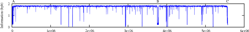
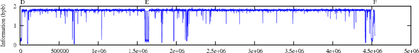
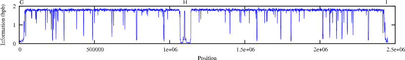
Figure 1: Plots of the information content for chromosome I (first row), chromosome II (second row) and chromosome III (third row) of S. pombe. The information profiles were obtained by processing the sequences in both directions, and then choosing the minimum information value in each direction. For better visualization, low-pass filtering with a Blackman window of $1,001$ bases was applied to the profiles.

In general, low-information regions are associated with the presence of repetitive sequences. For example, chromosome III has more and often more prominent low-information regions than chromosomes I and II, which is in compliance with some properties of this chromosome concerning repetitive structures, such as, the presence of tandem rDNA repeats [22] or the density of transposable element remnants in this chromosome being twice that of chromosomes I and II [23].

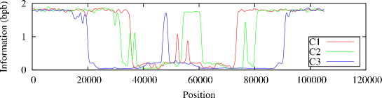
Figure 2: Plot of the information content of the centromeres of chromosome I (C1), II (C2) and III (C3).

We have also performed an inter-chromosomal study. We concatenated chromosome I with chromosome III and ran the algorithm from left to right and from right to left, picking the lowest information content values of both, base by base. A similar process has been done substituting chromosome I by II. Figure 3 shows only the information profile of chromosome III calculated taking into account the statistics of chromosome I, second row, and chromosome II, third row. We can see important regions marked with the letters A, B and C. The region marked with letter B contains the $2,529$ bases of gene eft202 (from base $537,326$ to $539,854$ in chromosome III). This gene is also present in chromosome I, named eft201, located from base $2,907,701$ to $2,910,229$, and has $\sim$99% sequence similarity to gene eft202.

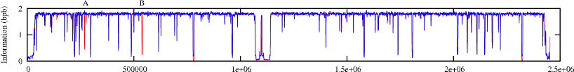
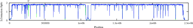
Figure 3: Information content of chromosome III of S. pombe. The first row shows a representation for chromosome III and their long repetitive zones. The second row shows chromosome III (blue) with information added from chromosome I (green). The third row shows chromosome III (blue) with information added from chromosome II (red).

The region marked with letter A in Fig. 3 indicates a region in chromosome III (gene ef1a-a) that is highly similar ($\sim$98% sequence similarity) with a region of chromosome I (gene ef1a-b). Although not included here, we found also an identical degree of similarity with gene ef1a-c in chromosome II. Fig. 4 illustrates the relative position of these genes, where letter A marks a region from base $4,095,202$ to $4,096,584$ ($1,383$ bases, chromosome I), letter B refers from base $626,106$ to $627,488$ ($1,383$ bases, chromosome II), and letter C from base $268,097$ to $269,479$ ($1,383$ bases, chromosome III).

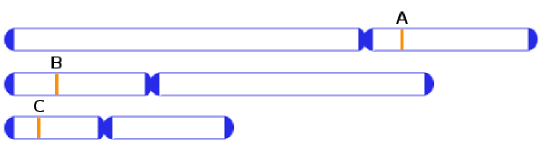
Figure 4: Illustration of the three chromosomes of S. pombe genome marked with genes ef1a-b (A), ef1a-c (B) and ef1a-a (C).

4 Conclusions

We described an algorithm to detect genomic regularities within a blind discovery strategy. This algorithm uses information profiles built using an efficient DNA sequence compression method. The results described support our claim that information profiles provide a valuable discovery tool for genome-wide studies. In fact, the accurate matching of the low-information regions to annotated repetitive genomic structures, such as the centromeric and telomeric regions of a chromosome, proves information profiles may be useful in de novo discovery of large-scale genomic regularities. Clearly, it is not possible to infer the genomic sequence per se from the information profiles, or the location of genomic regularities within base pair resolution. However, it is possible to discover the presence of regularities on a genome-wide scale, which may be useful for an exploratory genome analysis or for genome comparisons.

Our algorithm relies on the efficient probabilistic modeling of the genomic sequence based on finite-context models. The approach is sufficiently flexible and powerful to enable addressing various biological questions and quickly obtaining the corresponding information profiles for a first-hand assessment. Indeed, the creation of information profiles does not require high performance computational facilities. Building an information profile requires a computation time that depends only linearly on the size of the sequence. For example, the information profile of a human chromosome can be created in a laptop computer in just a few minutes. Moreover, the amount of computer memory required does not depend on the size of the sequence, but only on the depth of the finite context models used for modeling the sequence.

5 Acknowledgements

This work was supported in part by FEDER through the Operational Program Competitiveness Factors - COMPETE and by National Funds through FCT - Foundation for Science and Technology, in the context of the projects FCOMP-01-0124-FEDER-022682 (FCT reference PEst-C/EEI/UI0127/2011) and Incentivo/EEI/UI0127/2013.

6 References

References

- [1] T. D. Schneider and R. M. Stephens, “Sequence logos: a new way to display consensus sequences,” Nucleic Acids Research, vol. 18, no. 20, pp. 6097–6100, 1990.
- [2] H. J. Jeffrey, “Chaos game representation of gene structure,” Nucleic Acids Research, vol. 18, no. 8, pp. 2163–2170, 1990.
- [3] J. L. Oliver, P. Bernaola-Galván, J. Guerrero-García, and R. Román-Roldán, “Entropic profiles of DNA sequences through chaos-game-derived images,” Journal of Theoretical Biology, vol. 160, pp. 457–470, 1993.
- [4] N. Goldman, “Nucleotide, dinucleotide and trinucleotide frequencies explain patterns observed in chaos game representations of DNA sequences,” Nucleic Acids Research, vol. 21, no. 10, pp. 2487–2491, 1993.
- [5] L. J. Jensen, C. Friis, and D. W. Ussery, “Three views of microbial genomes,” Research in Microbiology, vol. 150, pp. 773–777, 1999.
- [6] P. J. Deschavanne, A. Giron, J. Vilain, G. Fagot, and B. Fertil, “Genomic signature: characterization and classification of species assessed by chaos game representation of sequences,” Molecular Biology and Evolution, vol. 16, no. 10, pp. 1391–1399, 1999.
- [7] M. Crochemore and R. Vérin, “Zones of low entropy in genomic sequences,” Computers & Chemistry, pp. 275–282, 1999.
- [8] O. G. Troyanskaya, O. Arbell, Y. Koren, G. M. Landau, and A. Bolshoy, “Sequence complexity profiles of prokaryotic genomic sequences: a fast algorithm for calculating linguistic complexity,” Bioinformatics, vol. 18, no. 5, pp. 679–688, 2002.
- [9] B. Fertil, M. Massin, S. Lespinats, C. Devic, P. Dumee, and A. Giron, “GENSTYLE: exploration and analysis of DNA sequences with genomic signature,” Nucleic Acids Research, vol. 33, pp. W512–W515, 2005.
- [10] S. Vinga and J. S. Almeida, “Local Renyi entropic profiles of DNA sequences,” BMC Bioinformatics, vol. 8, no. 393, 2007.
- [11] B. Clift, D. Haussler, R. McConnell, T. D. Schneider, and G. D. Stormo, “Sequence landscapes,” Nucleic Acids Research, vol. 14, no. 1, pp. 141–158, 1986.
- [12] L. Allison, L. Stern, T. Edgoose, and T. I. Dix, “Sequence complexity for biological sequence analysis,” Computers & Chemistry, vol. 24, pp. 43–55, 2000.
- [13] L. Stern, L. Allison, R. L. Coppel, and T. I. Dix, “Discovering patterns in Plasmodium falciparum genomic DNA,” Molecular & Biochemical Parasitology, vol. 118, pp. 174–186, 2001.
- [14] M. D. Cao, T. I. Dix, L. Allison, and C. Mears, “A simple statistical algorithm for biological sequence compression,” in Proc. of the Data Compression Conf., DCC-2007, Snowbird, Utah, Mar. 2007, pp. 43–52.
- [15] T. I. Dix, D. R. Powell, L. Allison, J. Bernal, S. Jaeger, and L. Stern, “Comparative analysis of long DNA sequences by per element information content using different contexts,” BMC Bioinformatics, vol. 8, no. Suppl. 2, p. S10, 2007.
- [16] S. Grumbach and F. Tahi, “Compression of DNA sequences,” in Proc. of the Data Compression Conf., DCC-93, Snowbird, Utah, 1993, pp. 340–350.
- [17] E. Rivals, O. Delgrange, J.-P. Delahaye, M. Dauchet, M.-O. Delorme, A. Hénaut, and E. Ollivier, “Detection of significant patterns by compression algorithms: the case of approximate tandem repeats in DNA sequences,” Computer Applications in the Biosciences, vol. 13, pp. 131–136, 1997.
- [18] A. J. Pinho, A. J. R. Neves, C. A. C. Bastos, and P. J. S. G. Ferreira, “DNA coding using finite-context models and arithmetic coding,” in Proc. of the IEEE Int. Conf. on Acoustics, Speech, and Signal Processing, ICASSP-2009, Taipei, Taiwan, Apr. 2009, pp. 1693–1696.
- [19] D. Pratas and A. J. Pinho, “Compressing the human genome using exclusively Markov models,” in Advances in Intelligent and Soft Computing, Proc. of the 5th Int. Conf. on Practical Applications of Computational Biology & Bioinformatics, PACBB 2011, vol. 93, Apr. 2011, pp. 213–220.
- [20] A. J. Pinho, D. Pratas, and P. J. S. G. Ferreira, “Bacteria DNA sequence compression using a mixture of finite-context models,” in Proc. of the IEEE Workshop on Statistical Signal Processing, Nice, France, Jun. 2011.
- [21] A. J. Pinho, P. J. S. G. Ferreira, A. J. R. Neves, and C. A. C. Bastos, “On the representability of complete genomes by multiple competing finite-context (Markov) models,” PLoS ONE, vol. 6, no. 6, p. e21588, 2011.
- [22] V. Wood, “Schizosaccharomyces pombe comparative genomics; from sequence to systems,” in Comparative Genomics, ser. Topics in Current Genetics, P. Sunnerhagen and J. Piskur, Eds. Springer-Verlag, 2006, vol. 15, pp. 233–285.
- [23] V. Wood et al., “The genome sequence of Schizosaccharomyces pombe,” Nature, vol. 415, no. 6874, pp. 871–80, Feb. 2002.