Adaptive Power Allocation Strategies using DSTC in Cooperative MIMO Networks

Abstract

Adaptive Power Allocation (PA) algorithms with different criteria for a cooperative Multiple-Input Multiple-Output (MIMO) network equipped with Distributed Space-Time Coding (DSTC) are proposed and evaluated. Joint constrained optimization algorithms to determine the power allocation parameters, the channel parameters and the receive filter are proposed for each transmitted stream in each link. Linear receive filter and maximum-likelihood (ML) detection are considered with Amplify-and-Forward (AF) and Decode-and-Forward (DF) cooperation strategies. In the proposed algorithms, the elements in the PA matrices are optimized at the destination node and then transmitted back to the relay nodes via a feedback channel. The effects of the feedback errors are considered. Linear MMSE expressions and the PA matrices depend on each other and are updated iteratively. Stochastic gradient (SG) algorithms are developed with reduced computational complexity. Simulation results show that the proposed algorithms obtain significant performance gains as compared to existing power allocation schemes.

I Introduction

Due to the benefits of cooperative multiple-input and multiple-output (MIMO) systems [1], extensive studies of cooperative MIMO networks have been undertaken [3]-[9]. In [3], an adaptive joint relay selection and power allocation algorithm based on the minimum mean square error (MMSE) criterion is designed. A joint transmit diversity optimization and relay selection algorithm for the Decode-and-Forward (DF) cooperating strategy [2] is designed in [4]. A transmit diversity selection matrix is introduced at each relay node in order to achieve a better MSE performance by deactivating some relay nodes. A central node which controls the transmission power for each link is employed in [6]. Although the centralized power allocation can improve the performance significantly, the complexity of the calculation increases with the size of the system. The works on the power allocation problem for the DF strategy measuring the outage probability in each relay node with a single antenna and determining the power for each link between the relay nodes and the destination node, have been reported in [12]-[14]. The diversity gain can be improved by using relay nodes with multiple antennas. When the number of relay nodes is the same, the cooperative gain can be improved by using the DF strategy compared with a system employing the AF strategy. However, the interference at the destination will be increased if the relay nodes forward the incorrectly detected symbols in the DF strategy. The power allocation optimization algorithms in [21] and [22] provide improved BER performance at the cost of requiring an eigenvalue decomposition to obtain the key parameters.

In this paper, we propose joint adaptive power allocation (JAPA) algorithms according to different optimization criteria with a linear receiver or an ML detector for cooperative MIMO systems employing multiple relay nodes with multiple antennas that perform cooperating strategies. This work was first introduced and discussed in [10] and [11]. The power allocation matrices utilized in [10] are full rank and after the optimization, all the parameters are transmitted back to the relay nodes and the source node with an error-free and delay-free feedback channel. In this paper, we employ the diagonal power allocation matrices in which the parameters stand for the power allocated to each transmit antenna. The requirement of the limited feedback is significantly reduced as compared to the algorithms in the previously reported works. It is worth to mention that the JAPA strategies derived in our algorithms are two-phase optimization techniques, which optimized the power assigned at the source node and at the relay nodes in the first phase and the second phase iteratively, and the proposed JAPA algorithms can be used as a power allocation strategy for the second phase only.

Three optimization criteria, namely, MMSE, minimum bit error rate (MBER) and maximum sum rate (MSR), are employed in the proposed JAPA optimization algorithms in this paper. We firstly develop joint optimization algorithms of the power allocation matrices and the linear receive filter according to these three criteria, respectively, which require matrix inversions and bring a high computational burden to the receiver. In the proposed JAPA algorithms with the MMSE, MBER, and MSR criteria, an SG method [15] is employed in order to reduce the computational complexity of the proposed algorithms. A comparison of the computational complexity of the algorithms is considered in this paper. A normalization procedure is employed by the optimization algorithm in order to enforce the power constraint in both transmission phases. After the normalization, the PA parameters are transmitted back to each transmit node through a feedback channel. The effect of the feedback errors is considered in the analysis and in the simulation sections, where we indicate an increased MSE performance due to feedback inaccuracy.

The paper is organized as follows. Section II introduces a two-hop cooperative MIMO system with multiple relays applying the AF strategy and the adaptive DSTC scheme. The constrained power allocation problems for relay nodes and linear detection method are derived in Section III, and the proposed JAPA SG algorithms are derived in Section IV. Section V focuses on the computational complexity comparison between the proposed and the existing algorithms, and the effects of the feedback errors on the MSE of the system. Section VI gives the simulation results and Section VII provides the conclusion.

Notation: the italic, bold lower-case and bold upper-case letters denote scalars, vectors and matrices, respectively. The operators $E[\cdot]$ and $(\cdot)^{\emph{H}}$ stand for expected value and the Hermitian operator. The $N\times N$ identity matrix is written as ${\boldsymbol{I}}_{N}$. $\parallel{\boldsymbol{X}}\parallel_{F}=\sqrt{{\rm Tr}({\boldsymbol{X}}^{H}\cdot{\boldsymbol{X}})}=\sqrt{{\rm Tr}({\boldsymbol{X}}\cdot{\boldsymbol{X}}^{\emph{H}})}$ is the Frobenius norm. $\Re[\cdot]$ stands for the real part, and $Tr(\cdot)$ stands for the trace of a matrix. $\rm{sgn}(\cdot)$ denotes the sign function.

II Cooperative System Model

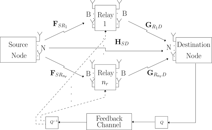
Figure 1: Cooperative MIMO system model with $n_{r}$ relay nodes

Consider a two-hop cooperative MIMO system in Fig. 1 with $n_{r}$ relay nodes that employs an AF cooperative strategy as well as a DSTC scheme. The source node and the destination node have $N$ antennas to transmit and receive data. An arbitrary number of antennas can be used at the relays which is denoted by $B$ shown in Fig. 1. We consider only one user at the source node in our system that operates in a spatial multiplexing configuration. Let ${\boldsymbol{s}}[i]$ denote the transmitted information symbol vector at the source node which contains $N$ symbols ${\boldsymbol{s}}[i]=[s_{1}[i],s_{2}[i],...,s_{N}[i]]$, and has a covariance matrix $E\big{[}{\boldsymbol{s}}[i]{\boldsymbol{s}}^{H}[i]\big{]}=\sigma_{s}^{2}{\boldsymbol{I}}_{N}$, where $\sigma_{s}^{2}$ is the signal power which we assume to be equal to 1. The source node broadcasts ${\boldsymbol{s}}[i]$ from the source to $n_{r}$ relay nodes as well as to the destination node in the first hop, which can be described by

$${\boldsymbol{r}}_{SD}[i]= {\boldsymbol{H}}_{SD}[i]{\boldsymbol{A}}_{S}[i]{\boldsymbol{s}}[i]+{\boldsymbol{n}}_{SD}[i],$$ (1)

$${\boldsymbol{r}}_{{SR}_{k}}[i]= {\boldsymbol{F}}_{SR_{k}}[i]{\boldsymbol{A}}_{S}[i]{\boldsymbol{s}}[i]+{\boldsymbol{n}}_{SR_{k}}[i],$$

$$k= 1,2,~{}...~{}n_{r},~{}~{}i=1,2,~{}...~{},$$

where ${\boldsymbol{A}}_{S}[i]=\rm{diag}[a_{S_{1}}[i],a_{S_{2}}[i],...,a_{S_{N}}[i]]$ denotes the diagonal $N\times N$ power allocation matrix assigned for the source node, and ${\boldsymbol{r}}_{{SR}_{k}}[i]$ and ${\boldsymbol{r}}_{SD}[i]$ denote the received symbol vectors at the $k$th relay node and at the destination node, respectively. The $B\times 1$ vectors ${\boldsymbol{n}}_{{SR}_{k}}[i]$ and ${\boldsymbol{n}}_{SD}[i]$ denote the zero mean complex circular symmetric additive white Gaussian noise (AWGN) vector generated at the $k$th relay node and at the destination node with variance $\sigma^{2}$. The matrices ${\boldsymbol{F}}_{SR_{k}}[i]$ and ${\boldsymbol{H}}_{SD}[i]$ are the $B\times N$ channel coefficient matrices. It is worth to mention that an orthogonal transmission protocol is considered which requires that the source node does not transmit during the time period of the second hop.

The received symbols are amplified and re-encoded at each relay node prior to transmission to the destination node in the second hop. We assume that the synchronization at each node is perfect. The received vector ${\boldsymbol{r}}_{SR_{k}}[i]$ at the $k$th relay node is assigned a $B\times B$ diagonal power allocation matrix ${\boldsymbol{A}}_{k}[i]=\rm{diag}[a_{k_{1}},a_{k_{2}},...,a_{k_{B}}]$ which leads to $\tilde{{\boldsymbol{s}}}_{SR_{k}}[i]={\boldsymbol{A}}_{k}[i]{\boldsymbol{r}}_{SR_{k}}[i]$. The $B\times 1$ signal vector $\tilde{{\boldsymbol{s}}}_{SR_{k}}[i]$ will be re-encoded by a $B\times T$ DSTC matrix ${\boldsymbol{M}}(\tilde{{\boldsymbol{s}}})$, and then forwarded to the destination node. The relationship between the $k$th relay and the destination node can be described as

$${\boldsymbol{R}}_{R_{k}D}[i]={\boldsymbol{G}}_{R_{k}D}[i]{\boldsymbol{M}}_{R_{k}D}[i]+{\boldsymbol{N}}_{RD}[i].$$ (2)

The $N\times T$ received symbol matrix ${\boldsymbol{R}}_{R_{k}D}[i]$ in (2) can be written as an $NT\times 1$ vector ${\boldsymbol{r}}_{R_{k}D}[i]$ given by

$${\boldsymbol{r}}_{R_{k}D}[i] ={\boldsymbol{G}}_{{eq}_{k}}[i]\tilde{{\boldsymbol{s}}}_{SR_{k}}[i]+{\boldsymbol{n}}_{R_{k}D}[i]={\boldsymbol{G}}_{{eq}_{k}}[i]{\boldsymbol{A}}_{k}[i]{\boldsymbol{r}}_{SR_{k}}[i]+{\boldsymbol{n}}_{RD}[i]$$ (3)

$$={\boldsymbol{G}}_{{eq}_{k}}[i]{\boldsymbol{A}}_{k}[i]{\boldsymbol{F}}_{SR_{k}}[i]{\boldsymbol{A}}_{S}[i]{\boldsymbol{s}}[i]+{\boldsymbol{n}}_{R_{k}}[i]+{\boldsymbol{n}}_{RD}[i],$$

where the $NT\times B$ matrix ${\boldsymbol{G}}_{eq_{k}}[i]$ stands for the equivalent channel matrix which is the DSTC scheme ${\boldsymbol{M}}(\tilde{{\boldsymbol{s}}}[i])$ combined with the channel matrix ${\boldsymbol{G}}_{R_{k}D}[i]$. The second term ${\boldsymbol{n}}_{R_{k}}[i]={\boldsymbol{G}}_{{eq}_{k}}[i]{\boldsymbol{A}}_{k}[i]{\boldsymbol{n}}_{SR_{k}}[i]$ in (3) stands for the amplified noise received from the relay node, and the $NT\times 1$ equivalent noise vector ${\boldsymbol{n}}_{RD}[i]$ generated at the destination node contains the noise parameters in ${\boldsymbol{N}}_{RD}[i]$.

After rewriting ${\boldsymbol{R}}_{R_{k}D}[i]$ we can consider the received symbol vector at the destination node as a $(T+1)N\times 1$ vector with two parts, one is from the source node and another one is the superposition of the received vectors from each relay node. Therefore, we can write the received symbol at the destination node as

$${\boldsymbol{r}}[i] =\left[\begin{array}[]{c}{\boldsymbol{r}}_{SD}[i]\\ {\boldsymbol{r}}_{RD}[i]\end{array}\right]=\left[\begin{array}[]{c}{\boldsymbol{H}}_{SD}[i]{\boldsymbol{A}}_{S}[i]{\boldsymbol{s}}[i]+{\boldsymbol{n}}_{SD}[i]\\ \sum_{k=1}^{n_{r}}{\boldsymbol{G}}_{{eq}_{k}}[i]{\boldsymbol{A}}_{k}[i]{\boldsymbol{F}}_{SR_{k}}[i]{\boldsymbol{A}}_{S}[i]{\boldsymbol{s}}[i]+{\boldsymbol{n}}_{RD}[i]\end{array}\right]=\left[\begin{array}[]{c}{\boldsymbol{H}}_{eq_{SD}}[i]\\ \sum_{k=1}^{n_{r}}{\boldsymbol{H}}_{{eq}_{k}}[i]\end{array}\right]{\boldsymbol{s}}[i]+\left[\begin{array}[]{c}{\boldsymbol{n}}_{SD}[i]\\ {\boldsymbol{n}}_{RD}[i]\end{array}\right]$$ (4)

$$={\boldsymbol{H}}_{D}[i]{\boldsymbol{s}}[i]+{\boldsymbol{n}}_{D}[i],$$

where the $(T+1)N\times N$ matrix ${\boldsymbol{H}}_{D}[i]$ denotes the channel gain matrix with the power allocation of all the links in the system. The $N\times N$ channel matrix ${\boldsymbol{H}}_{eq_{SD}}[i]={\boldsymbol{H}}_{SD}[i]{\boldsymbol{A}}_{S}[i]$, while the $k$th equivalent channel matrix ${\boldsymbol{H}}_{{eq}_{k}}[i]={\boldsymbol{G}}_{{eq}_{k}}[i]{\boldsymbol{A}}_{k}[i]{\boldsymbol{F}}_{SR_{k}}[i]{\boldsymbol{A}}_{S}[i]$. We assume that the coefficients in all channel matrices are statistically independent and remain constant over the transmission. The $(T+1)N\times 1$ noise vector ${\boldsymbol{n}}_{D}[i]$ contains the equivalent received noise vector at the destination node, which can be modeled as AWGN with zero mean and covariance matrix $\sigma^{2}(1+\parallel\sum_{k=1}^{n_{r}}{\boldsymbol{G}}_{{eq}_{k}}[i]{\boldsymbol{A}}_{k}[i]\parallel^{2}_{F}){\boldsymbol{I}}_{(T+1)N}$. It is worth to mention that the value in $B$ is variable and, in this work, we focus on the power allocation optimization algorithms in cooperative MIMO systems. For simplicity, we consider scenarios in which there are $B=N$ antennas at the relays.

III Adaptive Power Allocation Matrix Optimization Strategies

In this section, we consider the design of a two-phase adjustable power allocation matrix according to various criteria using a DSTC scheme in cooperative MIMO systems. The linear receive filter is determined jointly with the power allocation matrices. A feedback channel is considered in order to convey the information about the power allocation prior to transmission to the destination node.

III-A Joint Linear MMSE Receiver Design with Power Allocation

The linear MMSE receiver design with power allocation matrices is derived as follows. By defining the $(T+1)N\times 1$ parameter vector ${\boldsymbol{w}}_{j}[i]$ to determine the $j$th symbol $s_{j}[i]$ in the signal vector ${\boldsymbol{s}}[i]$, we propose the MSE based optimization with a power constraint described by

$$\left[{\boldsymbol{w}}_{j}[i],{\boldsymbol{A}}_{S}[i],{\boldsymbol{A}}_{k}[i]]\right]=\operatornamewithlimits{argmin}_{{\boldsymbol{w}}_{j}[i],{\boldsymbol{A}}_{S}[i],{\boldsymbol{A}}_{k}[i]}E\left[\|s_{j}[i]-{\boldsymbol{w}}_{j}^{\emph{H}}[i]{\boldsymbol{r}}[i]\|^{2}\right],$$ (5)

$$~{}~{}~{}~{}~{}~{}~{}~{}~{}s.t.~{}\rm{Tr}(\sum_{k=1}^{n_{r}}{\boldsymbol{A}}_{k}[i]{\boldsymbol{A}}_{k}^{\emph{H}}[i])\leq\rm{P_{R}},~{}\rm{Tr}({\boldsymbol{A}}_{S}[i]{\boldsymbol{A}}_{S}^{\emph{H}}[i])\leq\rm{P_{T}},$$

where $P_{T}$ and $P_{R}$ denote the transmit power assigned to all the relay nodes and to the source node, respectively. The values of the parameters in the power allocation (PA) matrices are restricted by $P_{T}$ and $P_{R}$. By employing the Lagrange multipliers $\lambda_{1}$ and $\lambda_{2}$ we can obtain the Lagrangian function shown as

$$\mathscr{L}=E\left[\|s_{j}[i]-{\boldsymbol{w}}_{j}^{\emph{H}}[i]{\boldsymbol{r}}[i]\|^{2}\right]+\lambda_{1}(\sum_{j=1}^{N}a_{S_{j}}[i]-P_{T})+\lambda_{2}(\sum_{k=1}^{n_{r}}\sum_{j=1}^{N}a_{k_{j}}[i]-P_{R}),$$ (6)

where $a_{S_{j}}[i]$ denotes the $j$th parameters in the diagonal of ${\boldsymbol{A}}_{S}[i]$ while $a_{k_{j}}[i]$ stands for the $j$th parameters in the diagonal of ${\boldsymbol{A}}_{k}[i]$.

By expanding the right-hand side of (6), taking the gradient with respect to ${\boldsymbol{w}}_{j}^{*}[i]$, $a^{*}_{S_{j}}[i]$ and $a^{*}_{k_{j}}[i]$, respectively, and equating the terms to zero, we can obtain

$${\boldsymbol{w}}_{j}[i] ={\boldsymbol{R}}^{-1}{\boldsymbol{p}},$$ (7)

$$a_{S_{j}}[i] =\tilde{R}^{-1}_{S}\tilde{P}_{S},$$

$$a_{k_{j}}[i] =\tilde{R}^{-1}\tilde{P},$$

where

$${\boldsymbol{R}} =E\left[{\boldsymbol{r}}[i]{\boldsymbol{r}}^{\emph{H}}[i]\right],~{}{\boldsymbol{p}}=E\left[{\boldsymbol{r}}[i]s_{j}^{*}[i]\right],$$ (8)

$$\tilde{R}_{S} =E\left[{\boldsymbol{w}}^{\emph{H}}_{j}[i]{\boldsymbol{h}}_{{SDA}_{j}}[i]s_{j}[i]s^{*}_{j}[i]{\boldsymbol{h}}^{\emph{H}}_{{SDA}_{j}}[i]{\boldsymbol{w}}_{j}[i]+\lambda_{1}a_{S_{j}}[i]\right],$$

$$\tilde{P}_{S} =E\left[{\boldsymbol{h}}^{\emph{H}}_{{SDA}_{j}}[i]{\boldsymbol{w}}_{j}[i]s^{*}_{j}[i]s_{j}[i]\right],$$

$$\tilde{P} =E\left[s_{j}[i]s^{*}_{j}[i]a_{S_{j}}^{*}[i]f^{*}_{k_{j}}[i]{\boldsymbol{g}}^{\emph{H}}_{eq_{k_{j}}}[i]{\boldsymbol{w}}_{j}[i]\right],$$

$$\tilde{R} =E\left[{\boldsymbol{w}}^{\emph{H}}_{j}[i]{\boldsymbol{g}}_{eq_{k_{j}}}[i]f_{k_{j}}[i]a_{S_{j}}[i]s_{j}[i]s^{*}_{j}[i]a_{S_{j}}^{*}[i]f^{*}_{k_{j}}[i]{\boldsymbol{g}}^{\emph{H}}_{eq_{k_{j}}}[i]{\boldsymbol{w}}_{j}[i]+\lambda_{2}a_{k_{j}}[i]\right].$$

The vector ${\boldsymbol{h}}_{SDA_{j}}$ denotes the channel vector assigned to the parameter $a_{S_{j}}$ and is the $j$th column of the equivalent channel matrix ${\boldsymbol{H}}_{SDA}[i]=\left[{\boldsymbol{H}}_{SD}[i];{\boldsymbol{G}}_{{eq}_{k}}[i]{\boldsymbol{A}}_{k}[i]{\boldsymbol{F}}_{SR_{k}}[i]\right]$ , and $f_{k_{j}}[i]$ and ${\boldsymbol{g}}_{eq_{k_{j}}}[i]$ denotes the $j$th parameter in ${\boldsymbol{F}}_{k}[i]$ and the $j$th column in ${\boldsymbol{G}}_{eq_{k}}[i]$, respectively. The value of the Lagrange multipliers $\lambda_{1}$ and $\lambda_{2}$ can be determined by substituting ${\boldsymbol{A}}_{S}[i]$ and ${\boldsymbol{A}}_{k}[i]$ into $\rm{Tr}({\boldsymbol{A}}_{S}[i]{\boldsymbol{A}}_{S}^{\emph{H}}[i])\leq\rm{P_{T}}$ and $\lambda\rm{Tr}(\sum_{k=1}^{n_{r}}{\boldsymbol{A}}_{k}[i]{\boldsymbol{A}}^{\emph{H}}_{k}[i])=\rm{P_{R}}$, respectively, and then solving the power constraint equations. The problem is that a high computational complexity of ${\rm O}(((T+1)N)^{3})$ is required, and it will increase cubically with the number of antennas or the use of more complicated STC encoders.

III-B Joint Linear MBER Receiver Design with Power Allocation

The MBER receiver design [17, 18] with power allocation in the second phase is derived as follows. The BPSK modulation scheme is utilized for simplicity. According to the expression in (4), the desired information symbols at the destination node can be computed as

$$b_{j}[i]=\rm{sgn}({\boldsymbol{w}}^{\emph{H}}_{j}[i]{\boldsymbol{r}}[i])=\rm{sgn}(\tilde{s}_{j}[i]),$$ (9)

where $\tilde{s}_{j}[i]$ denotes the detected symbol at the receiver which can be further written as

$$\tilde{s}_{j}[i] =\Re\left[{\boldsymbol{w}}^{\emph{H}}_{j}[i]{\boldsymbol{r}}[i]\right]=\Re\left[{\boldsymbol{w}}^{\emph{H}}_{j}[i]({\boldsymbol{H}}_{D}[i]{\boldsymbol{s}}[i]+{\boldsymbol{n}}_{D}[i])\right]=\Re\left[{\boldsymbol{w}}^{\emph{H}}_{j}[i]{\boldsymbol{H}}_{D}[i]{\boldsymbol{s}}[i]+{\boldsymbol{w}}^{\emph{H}}_{j}[i]{\boldsymbol{n}}_{D}[i]\right]$$ (10)

$$=\Re\left[\tilde{s}^{\prime}_{j}[i]+e_{j}[i]\right],$$

where $\tilde{s}^{\prime}_{j}[i]$ is the noise-free detected symbol, and $e_{j}[i]$ denotes the error factor for the $j$th detected symbol. Define an $N\times N_{b}$ matrix $\boldsymbol{\bar{S}}$ which is constructed by a set of vectors ${\boldsymbol{\bar{s}}}_{l}=[s_{l_{1}},s_{l_{2}},...,s_{l_{N}}]^{T},~{}l=1,2,...,N_{b}$ and $N_{b}=2^{N}$, containing all the possible combinations of the transmitted symbol vector ${\boldsymbol{s}}[i]$ and we can obtain

$${\bar{s}}_{l_{j}}[i]=\Re\left[{\boldsymbol{w}}^{\emph{H}}_{j}[i]{\boldsymbol{H}}_{D}[i]{\boldsymbol{\bar{s}}}_{l}+{\boldsymbol{w}}^{\emph{H}}_{j}[i]{\boldsymbol{n}}_{D}[i]\right]=\Re\left[{\boldsymbol{w}}^{\emph{H}}_{j}[i]\boldsymbol{\bar{r}}_{l}[i]]+e_{l_{j}}[i]\right]=\bar{s}^{\prime}_{l_{j}}[i]+e_{l_{j}}[i],$$ (11)

where $\bar{s}^{\prime}_{l_{j}}[i]$ denotes the noise-free detected symbol in the $l$th column and the $j$th row of ${\boldsymbol{\bar{S}}}$. Since the probability density function (pdf) of $\boldsymbol{\bar{r}}[i]$ is given by

$$p_{\boldsymbol{\bar{r}}[i]}=\frac{1}{N_{b}\sqrt{2\pi\sigma^{2}_{n}{\boldsymbol{w}}^{\emph{H}}_{j}[i]{\boldsymbol{w}}_{j}[i]}}\sum_{l=1}^{N_{b}}\exp\big{(}-\frac{(\bar{s}_{l_{j}}[i]-\bar{s}^{\prime}_{l_{j}}[i])^{2}}{2\sigma^{2}_{n}{\boldsymbol{w}}^{\emph{H}}_{j}[i]{\boldsymbol{w}}_{j}[i]}\big{)},$$ (12)

by employing the $Q$ function, we can obtain the BER expression of the cooperative MIMO system which is

$$P_{E}({\boldsymbol{w}}_{j}[i],a_{S_{j}}[i],a_{k_{j}}[i])=\frac{1}{N_{b}}\sum^{N_{b}}_{l=1}{\boldsymbol{Q}}(c_{l_{j}}[i]),$$ (13)

where

$$c_{l_{j}}[i]=\frac{sgn(s_{l_{j}})\bar{s}_{l_{j}}^{\prime}[i]}{\sigma_{n}\sqrt{{\boldsymbol{w}}^{\emph{H}}_{j}[i]{\boldsymbol{w}}_{j}[i]}}=\frac{sgn(s_{l_{j}})\Re\left[{\boldsymbol{w}}^{\emph{H}}_{j}[i]\boldsymbol{\bar{r}}_{l}[i]\right]}{\sigma_{n}\sqrt{{\boldsymbol{w}}^{\emph{H}}_{j}[i]{\boldsymbol{w}}_{j}[i]}}.$$ (14)

The joint power allocation with linear receiver design problem is given by

$$[{\boldsymbol{w}}_{j}[i],a_{S_{j}}[i],a_{k_{j}}[i]]=\operatornamewithlimits{argmin}_{{\boldsymbol{w}}_{j}[i],a_{S_{j}}[i],a_{k_{j}}[i]}P_{E}({\boldsymbol{w}}_{j}[i],a_{S_{j}}[i],a_{k_{j}}[i]),$$ (15)

$$~{}~{}~{}~{}~{}~{}~{}~{}~{}s.t.~{}\sum_{j=1}^{N}a_{S_{j}}[i]\leq\rm{P_{T}},~{}\sum_{k=1}^{n_{r}}\sum_{j=1}^{N}a_{k_{j}}[i]\leq\rm{P_{R}}.$$

According to (13) and (14), the solution of the design problem in (15) with respect to ${\boldsymbol{w}}_{j}[i]$, $a_{S_{j}}[i]$ and $a_{k_{j}}[i]$ is not a closed-form one. Therefore, we design an adaptive JAPA strategy according to the MBER criterion using the SG algorithm in order to update the parameters iteratively to achieve the optimal solution in the next section.

III-C Joint Linear MSR Receiver Design with Power Allocation

We will develop a joint power allocation strategy focuses on maximizing the sum rate at the destination node. The expression of the sum rate after the detection is derived in [19] as

$$I=\frac{1}{2}\log_{2}(1+SNR_{ins}),$$ (16)

where

$$SNR_{ins}=\frac{E[{\boldsymbol{s}}^{\emph{H}}{\boldsymbol{s}}]Tr({\boldsymbol{W}}^{\emph{H}}[i]{\boldsymbol{H}}_{D}[i]{\boldsymbol{H}}^{\emph{H}}_{D}[i]{\boldsymbol{W}}[i])}{E[{\boldsymbol{n}}^{\emph{H}}_{D}[i]{\boldsymbol{n}}_{D}[i]]},$$ (17)

and ${\boldsymbol{W}}[i]=[{\boldsymbol{w}}_{1}[i],{\boldsymbol{w}}_{2}[i],...,{\boldsymbol{w}}_{N}[i]]$ denotes the $N(T+1)\times N$ linear receive filter matrix, and ${\boldsymbol{n}}[i]$ denotes the received noise vector. By substituting (4) into (17), we can obtain

$$SNR_{ins}=\frac{\sigma^{2}_{s}Tr({\boldsymbol{W}}^{\emph{H}}[i](\sum_{k=1}^{n_{r}}{\boldsymbol{G}}_{{eq}_{k}}[i]{\boldsymbol{A}}_{k}[i]{\boldsymbol{F}}_{SR_{k}}[i]{\boldsymbol{A}}_{S}[i])(\sum_{k=1}^{n_{r}}{\boldsymbol{G}}_{{eq}_{k}}[i]{\boldsymbol{A}}_{k}[i]{\boldsymbol{F}}_{SR_{k}}[i]{\boldsymbol{A}}_{S}[i])^{\emph{H}}{\boldsymbol{W}}[i])}{\sigma^{2}_{n}Tr({\boldsymbol{W}}^{\emph{H}}[i]({\boldsymbol{I}}_{N(T+1)}+(\sum_{k=1}^{n_{r}}{\boldsymbol{G}}_{{eq}_{k}}[i]{\boldsymbol{A}}_{R_{k}D}[i])(\sum_{k=1}^{n_{r}}{\boldsymbol{G}}_{{eq}_{k}}[i]{\boldsymbol{A}}_{R_{k}D}[i])^{\emph{H}}){\boldsymbol{W}}[i])}.$$ (18)

Since the logarithm is an increasing function, maximizing the sum rate is equivalent to maximizing the instantaneous SNR. The optimization problem can be written as

$$\left[{\boldsymbol{W}}[i],{\boldsymbol{A}}_{S}[i],{\boldsymbol{A}}_{k}[i]\right]=\operatornamewithlimits{argmax}_{{\boldsymbol{W}}[i],{\boldsymbol{A}}_{S}[i],{\boldsymbol{A}}_{k}[i]}SNR_{ins},~{}s.t.~{}\rm{Tr}({\boldsymbol{A}}_{k}[i]{\boldsymbol{A}}_{k}^{\emph{H}}[i])\leq\rm{P_{R}},~{}\rm{Tr}({\boldsymbol{A}}_{S}[i]{\boldsymbol{A}}_{S}^{\emph{H}}[i])\leq\rm{P_{T}},$$ (19)

where $SNR_{ins}$ is given by (18).

As expressed in (18), the solution of (19) with respect to the matrices ${\boldsymbol{W}}[i]$, ${\boldsymbol{A}}_{S}[i]$ and ${\boldsymbol{A}}_{k}[i]$ does not result in closed-form expressions. Therefore, in the next section we propose a JAPA SG algorithm to obtain the joint optimization algorithm for determining the linear receiver filter parameters and power allocation matrices to maximize the sum rate.

IV Low Complexity Joint Linear Receiver Design with Power Allocation

In this section, we jointly design an adjustable power allocation matrix and the linear receiver for the DSTC scheme in cooperative MIMO systems. Adaptive SG algorithms [15] with reduced complexity are devised.

IV-A Joint Adaptive SG Estimation for MMSE Receive Filter and Power Allocation

According to (5) and (6), the joint optimization problem for power allocation matrices and receiver parameter vectors depend on each other. By computing the instantaneous gradient terms of (6) with respect to ${\boldsymbol{w}}_{j}[i]$, $a_{S_{j}}[i]$ and $a_{k_{j}}[i]$, respectively, we can obtain

$$\nabla\mathscr{L}_{{\boldsymbol{w}}^{*}_{j}[i]} =-{\boldsymbol{r}}[i](s_{j}[i]-{\boldsymbol{w}}^{\emph{H}}_{j}[i]{\boldsymbol{r}}[i]))^{*}=-{\boldsymbol{r}}[i]e^{*}_{j}[i],$$ (20)

$$\nabla\mathscr{L}_{a^{*}_{S_{j}}[i]} =-\nabla_{a^{*}_{S_{j}}[i]}({\boldsymbol{w}}^{\emph{H}}_{j}[i]{\boldsymbol{h}}_{{SDA}_{j}}[i]a_{S_{j}}[i]s_{j}[i])^{\emph{H}}(s_{j}[i]-{\boldsymbol{w}}^{\emph{H}}_{j}[i]{\boldsymbol{r}}[i])={\boldsymbol{h}}^{\emph{H}}_{{SDA}_{j}}[i]{\boldsymbol{w}}_{j}[i]s^{*}_{j}[i]e_{j}[i],$$

$$\nabla\mathscr{L}_{a^{*}_{k_{j}}[i]} =-\nabla_{a^{*}_{k_{j}}[i]}({\boldsymbol{w}}^{\emph{H}}_{R_{j}}[i]{\boldsymbol{g}}_{eq_{k_{j}}}[i]{\boldsymbol{f}}_{k_{j}}[i]a_{k_{j}}[i]{\boldsymbol{s}}[i])^{\emph{H}}(s_{j}[i]-{\boldsymbol{w}}^{\emph{H}}_{j}[i]{\boldsymbol{r}}[i])=-({\boldsymbol{g}}_{eq_{k_{j}}}[i]{\boldsymbol{f}}_{k_{j}}[i]{\boldsymbol{s}}[i])^{\emph{H}}{\boldsymbol{w}}_{R_{j}}[i]e_{j}[i],$$

where ${\boldsymbol{h}}_{{SDA}_{j}}[i]$ denotes the $j$th column with dimension $N(T+1)\times 1$ of the equivalent channel matrix ${\boldsymbol{H}}_{SDA}[i]$, and ${\boldsymbol{g}}_{{eq_{k}}_{j}}[i]$ and ${\boldsymbol{f}}_{k_{j}}[i]$ denote the $j$th column and the $j$th row of the channel matrices ${\boldsymbol{F}}_{k}[i]$ and ${\boldsymbol{G}}_{eq_{k_{j}}}[i]$, respectively. The $NT\times 1$ vector ${\boldsymbol{w}}_{R_{j}}[i]$ is the parameter vector for the received symbols from the relay nodes. The error signal is denoted by $e_{j}[i]=s_{j}[i]-{\boldsymbol{w}}_{j}^{H}[i]{\boldsymbol{r}}[i]$. We can devise an adaptive SG estimation algorithm by using the instantaneous gradient terms of the Lagrangian which were previously derived with SG descent rules [15]:

$${\boldsymbol{w}}_{j}[i+1] ={\boldsymbol{w}}_{j}[i]-\mu\nabla\mathscr{L}_{{\boldsymbol{w}}^{*}_{j}[i]},$$ (21)

$$a_{S_{j}}[i+1] =a_{S_{j}}[i]-\nu\nabla\mathscr{L}_{a^{*}_{S_{j}}[i]},$$

$$a_{k_{j}}[i+1] =a_{k_{j}}[i]-\tau\nabla\mathscr{L}_{a^{*}_{k_{j}}[i]},$$

where $\mu$, $\nu$ and $\tau$ are the step sizes of the recursions for the estimation procedure. The computational complexity of ${\boldsymbol{w}}_{j}[i]$, $a_{S_{j}}[i]$ and $a_{k_{j}}[i]$ in (21) is $(\boldsymbol{O}(NT))$, $(\boldsymbol{O}(3NT))$ and $(\boldsymbol{O}(N^{2}T^{2}))$, respectively, which is much less than that of the algorithm we described in Section III.

It is worth to mention that instead of calculating the Lagrange multiplier $\lambda$, a normalization of the power allocation matrices after the optimization which ensures that the energy is not increased is required and implemented as

$${\boldsymbol{A}}_{S}[i+1]= \frac{\sqrt{\rm{P_{T}}}{\boldsymbol{A}}_{S}[i+1]}{\parallel{\boldsymbol{A}}_{S}[i+1]\parallel_{F}},$$ (22)

$${\boldsymbol{A}}_{k}[i+1]= \frac{\sqrt{\rm{P_{R}}}{\boldsymbol{A}}_{k}[i+1]}{\parallel\sum_{k=1}^{n_{r}}\rm{Tr}({\boldsymbol{A}}_{k}[i+1]\parallel_{F}}.$$

IV-B Joint Adaptive MBER SG Estimation and Power Allocation

The key strategy to derive an adaptive estimation algorithm for solving (15) is to find out an efficient and reliable method to calculate the pdf of the received symbol vector ${\boldsymbol{r}}[i]$ at the destination node. According to the algorithms in [16], kernel density estimation provides an effective method for accurately estimating the required pdf.

By transmitting a block of $M$ training samples ${\boldsymbol{\hat{s}}}=\rm{sgn}({\boldsymbol{\hat{b}}})$, the kernel density estimated pdf of ${\boldsymbol{\hat{s}}}[i]$ is given by

$$p_{\hat{s}}=\frac{1}{M\sqrt{2\pi}\rho_{n}\sqrt{{\boldsymbol{w}}^{\emph{H}}_{j}[i]{\boldsymbol{w}}_{j}[i]}}\sum_{j=1}^{M}exp\big{(}-\frac{(\tilde{s}_{j}-\hat{s}_{j})^{2}}{2\rho^{2}_{n}{\boldsymbol{w}}^{\emph{H}}_{j}[i]{\boldsymbol{w}}_{j}[i]}\big{)},$$ (23)

where $\rho_{n}$ is related to the standard deviation of noise $\sigma_{n}$ and it is suggested in [16] that a lower bound of $\rho_{n}=\big{(}\frac{4}{3M}\big{)}^{\frac{1}{5}}\sigma_{n}$ should be chosen. The symbol $\tilde{s}_{j}$ is calculated by (11), and $\hat{s}_{j}$ stands for the $j$th element in the $M\times 1$ training samples ${\boldsymbol{\hat{s}}}$. The expression of the BER can be derived as

$$\hat{P_{E}}({\boldsymbol{w}}_{j}[i],a_{S_{j}}[i],a_{k_{j}}[i])=\frac{1}{M}\sum^{M}_{j=1}{\boldsymbol{Q}}(c_{j}[i]),$$ (24)

where

$$c_{j}[i]=\frac{sgn(\hat{s}_{j})\bar{\hat{s}}_{j}}{\rho_{n}\sqrt{{\boldsymbol{w}}^{\emph{H}}_{j}[i]{\boldsymbol{w}}_{j}[i]}}.$$ (25)

By substituting (25) into (24) and taking the gradient with respect to different arguments, we can obtain

$$\nabla P_{E_{{\boldsymbol{w}}_{j}}}[i]=\frac{1}{M\sqrt{2\pi}\sqrt{{\boldsymbol{w}}^{\emph{H}}_{j}[i]{\boldsymbol{w}}_{j}[i]}}\sum^{M}_{j=1}\exp\big{(}-\frac{c^{2}_{j}[i]}{2}\big{)}sgn(s_{j})\frac{{\boldsymbol{\bar{r}}}[i]-\frac{1}{2}\bar{s}_{j}[i]{\boldsymbol{w}}_{j}[i]}{\sigma_{n}{\boldsymbol{w}}^{\emph{H}}_{j}[i]{\boldsymbol{w}}_{j}[i]},$$ (26)

$$\nabla P_{E_{a_{S_{j}}}}[i]=\frac{1}{M\sqrt{2\pi}\sigma_{n}\sqrt{{\boldsymbol{w}}^{\emph{H}}_{j}[i]{\boldsymbol{w}}_{j}[i]}}\sum^{M}_{j=1}exp\big{(}-\frac{c^{2}_{j}[i]}{2}\big{)}sgn(s_{j})\Re[{\boldsymbol{w}}^{\emph{H}}_{j}[i]{\boldsymbol{h}}_{SDA_{j}}[i]s_{j}],$$ (27)

$$\nabla P_{E_{a_{k_{j}}}}[i]=\frac{1}{M\sqrt{2\pi}\sigma_{n}\sqrt{{\boldsymbol{w}}^{\emph{H}}_{D_{j}}[i]{\boldsymbol{w}}_{R_{j}}[i]}}\sum^{M}_{j=1}exp\big{(}-\frac{c^{2}_{j}[i]}{2}\big{)}sgn(s_{j})\Re[{\boldsymbol{w}}^{\emph{H}}_{R_{j}}[i]{\boldsymbol{h}}_{k_{j}}[i]s_{j}],$$ (28)

where ${\boldsymbol{h}}_{k_{j}}[i]={\boldsymbol{g}}_{eq_{k_{j}}}[i]f_{k_{j}}[i]$ denotes the equivalent channel vector assigned for $s_{m_{j}}$. By making use of an SG algorithm in [15], the updated ${\boldsymbol{w}}_{j}[i]$, $a_{S_{j}}[i]$ and$a_{k_{j}}[i]$ can be calculated by (21). The convergence property of the joint iterative optimization problems have been tested and proved by Niesen et al. in [20]. In the proposed design problem the receive filter parameter vectors and the power allocation parameters depend on each other, and the proposed JAPA algorithms provide an iterative update process and finally both of the desired items will reach at least a local optimum of the BER cost function.

IV-C Joint Adaptive MSR SG Algorithm for Power Allocation and Receiver Design

The proposed power allocation algorithm that maximizes the sum rate at the destination node is derived as follows. We consider the design problem in (19) and the instantaneous received $SNR_{ins}$ as given in (18). According to the property of the trace $\rm{Tr}(\cdot)$ we can obtain

$$SNR_{ins}=\frac{\sigma^{2}_{s}}{n_{eq}[i]}Tr({\boldsymbol{R}}_{SDA}[i]{\boldsymbol{A}}^{\emph{H}}_{S}[i])=\frac{\sigma^{2}_{s}}{n_{eq}[i]}Tr(\sum_{k=1}^{n_{r}}{\boldsymbol{R}}_{{\boldsymbol{G}}_{eq_{k}}}[i]{\boldsymbol{A}}^{\emph{H}}_{k}[i]),$$ (29)

where

$${\boldsymbol{R}}_{SDA}[i]={\boldsymbol{H}}^{\emph{H}}_{SDA}[i]{\boldsymbol{W}}[i]{\boldsymbol{W}}^{\emph{H}}[i]{\boldsymbol{H}}_{SDA}[i]{\boldsymbol{A}}_{S}[i],$$

$${\boldsymbol{R}}_{{\boldsymbol{G}}_{eq_{k}}}[i]={\boldsymbol{G}}^{\emph{H}}_{eq_{k}}[i]{\boldsymbol{W}}[i]{\boldsymbol{W}}^{\emph{H}}[i]{\boldsymbol{H}}_{SDA}[i]{\boldsymbol{A}}_{S}[i]{\boldsymbol{A}}_{S}^{\emph{H}}[i]{\boldsymbol{F}}_{SR_{k}}^{\emph{H}}[i],$$

$$n_{eq}[i]=\sigma^{2}_{n}Tr({\boldsymbol{W}}^{\emph{H}}[i]{\boldsymbol{W}}[i]+{\boldsymbol{W}}^{\emph{H}}[i](\sum_{k=1}^{n_{r}}{\boldsymbol{G}}_{eq_{k}}[i]{\boldsymbol{A}}_{k}[i])(\sum_{k=1}^{n_{r}}{\boldsymbol{G}}_{eq_{k}}[i]{\boldsymbol{A}}_{k}[i])^{\emph{H}}{\boldsymbol{W}}[i]).$$

Since the power allocation matrices ${\boldsymbol{A}}_{S}[i]$ and ${\boldsymbol{A}}_{k}[i]$ are diagonal, we just focus on the terms containing the conjugate of the $j$th parameter in order to simplify the derivation, and rewrite (29) as

$$SNR_{ins}=\frac{\sigma^{2}_{s}\sum_{k=1}^{n_{r}}\sum_{j=1}^{N}r_{SDA_{j}}[i]a^{*}_{S_{j}}[i]}{\sigma^{2}_{n}\sum_{j=1}^{N}({\boldsymbol{w}}^{\emph{H}}_{j}[i]{\boldsymbol{w}}_{j}[i]+\sum_{k=1}^{n_{r}}r_{{{\boldsymbol{N}}_{k}}_{j}}[i]a^{*}_{k_{j}}[i])}=\frac{\sigma^{2}_{s}\sum_{k=1}^{n_{r}}\sum_{j=1}^{N}r_{{\boldsymbol{G}}_{eq_{k_{j}}}}[i]a^{*}_{k_{j}}[i]}{\sigma^{2}_{n}\sum_{j=1}^{N}({\boldsymbol{w}}^{\emph{H}}_{j}[i]{\boldsymbol{w}}_{j}[i]+\sum_{k=1}^{n_{r}}r_{{{\boldsymbol{N}}_{k}}_{j}}[i]a^{*}_{k_{j}}[i])},$$ (30)

where $r_{{\boldsymbol{G}}_{eq_{k_{j}}}}[i]$ and $r_{{{\boldsymbol{N}}_{k}}_{j}}[i]$ denotes the $j$th element in the diagonal of ${\boldsymbol{R}}_{{\boldsymbol{G}}_{eq_{k}}}[i]$ and ${\boldsymbol{R}}_{{\boldsymbol{N}}_{k}}[i]$, respectively. ${\boldsymbol{R}}_{{\boldsymbol{N}}_{k}}[i]={\boldsymbol{G}}^{\emph{H}}_{eq_{k}}[i]{\boldsymbol{W}}[i]{\boldsymbol{W}}^{\emph{H}}[i]{\boldsymbol{G}}_{eq_{k}}[i]{\boldsymbol{A}}_{k}[i]$ denotes the equivalent matrix assigned for the noise at the $k$th relay node.

By taking the stochastic gradient of (30) with respect to $a^{*}_{S_{j}}[i]$, $a^{*}_{k_{j}}[i]$ and ${\boldsymbol{W}}^{\emph{H}}[i]$ we can obtain

$$\nabla_{{\boldsymbol{W}}[i]} =\frac{\sigma^{2}_{s}}{n_{eq}[i]}(Tr(\parallel{\boldsymbol{H}}_{SDA}[i]{\boldsymbol{A}}_{S}[i]\parallel^{2}_{F}{\boldsymbol{W}}[i])n_{eq}[i]$$ (31)

$$~{}~{}~{}~{}~{}~{}~{}-\parallel{\boldsymbol{W}}^{\emph{H}}[i]{\boldsymbol{H}}_{SDA}[i]{\boldsymbol{A}}_{S}[i]\parallel^{2}_{F}Tr({\boldsymbol{W}}[i]+{\boldsymbol{G}}_{eq_{k}}[i]{\boldsymbol{A}}_{k}[i]({\boldsymbol{G}}_{eq_{k}}[i]{\boldsymbol{A}}_{k}[i]){\boldsymbol{W}}[i])),$$

$$\nabla_{a_{S_{j}}[i]} =\frac{\sigma^{2}_{s}}{n_{eq}[i]}r_{SDA_{j}}[i],$$

$$\nabla_{a_{R_{k}D}[i]} =\frac{\sigma^{2}_{s}}{n_{eq}[i]}(r_{{\boldsymbol{G}}_{eq}}[i]n_{eq}[i]-\sigma^{2}_{n}r_{{{\boldsymbol{N}}_{k}}_{j}}[i]\sum_{j=1}^{N}r_{{\boldsymbol{G}}_{eq_{k_{j}}}}[i]a^{*}_{k_{j}}[i]).$$

By using (21) and (22) the proposed algorithm is achieved. Table I shows a summary of the JAPA SG algorithms with different criteria. A low complexity channel estimation method derived in [10] can be also employed to obtain the channel matrices required in the proposed algorithms.

TABLE I: The JAPA SG Algorithms

1: Initialization:

${\boldsymbol{W}}[0]={\boldsymbol{I}}_{(T+1)N\times 1}$,

$a_{S_{j}}[0]=1,~{}a_{k_{j}}[0]=1$,

${\boldsymbol{H}}_{SDA}[i]=\sum_{k=1}^{n_{r}}{\boldsymbol{G}}_{eq_{k}}[i]{\boldsymbol{A}}_{k}[i]{\boldsymbol{F}}_{SR_{k}}[i]$,

2: for $j=1$ to $N$ do

2-1: JAPA SG MMSE Algorithm

$e_{j}[i]=s_{j}[i]-{\boldsymbol{w}}^{\emph{H}}_{j}[i]{\boldsymbol{r}}[i],$

$\nabla\mathscr{L}_{{\boldsymbol{w}}^{\emph{H}}_{j}[i]}=-{\boldsymbol{r}}[i]e^{*}_{j}[i],$

$\nabla\mathscr{L}_{a^{*}_{S_{j}}[i]}={\boldsymbol{h}}^{\emph{H}}_{{SDA}_{j}}[i]{\boldsymbol{w}}_{j}[i]s^{*}_{j}[i]e_{j}[i],$

$\nabla\mathscr{L}_{a^{*}_{k_{j}}[i]}=-({\boldsymbol{g}}_{eq_{k_{j}}}[i]{\boldsymbol{f}}_{k_{j}}[i]{\boldsymbol{s}}[i])^{\emph{H}}{\boldsymbol{w}}_{D_{j}}[i]e_{j}[i],$

2-2: JAPA SG MBER Algorithm

$c_{m_{j}}[i]=\frac{sgn(\hat{s}_{m_{j}})\bar{\hat{s}}_{m_{j}}}{\rho_{n}\sqrt{{\boldsymbol{w}}^{\emph{H}}_{j}[i]{\boldsymbol{w}}_{j}[i]}},~{}{\boldsymbol{h}}_{k_{j}}[i]={\boldsymbol{g}}_{eq_{k_{j}}}[i]f_{k_{j}}[i]$

$\nabla P_{E_{{\boldsymbol{w}}_{j}}}[i]=\frac{1}{M\sqrt{2\pi}\sqrt{{\boldsymbol{w}}^{\emph{H}}_{j}[i]{\boldsymbol{w}}_{j}[i]}}\sum^{M}_{j=1}\exp\big{(}-\frac{c^{2}_{j}[i]}{2}\big{)}sgn(s_{j})\frac{{\boldsymbol{\bar{r}_{j}}}[i]-\frac{1}{2}\bar{s}_{j}[i]{\boldsymbol{w}}_{j}[i]}{\sigma_{n}{\boldsymbol{w}}^{\emph{H}}_{j}[i]{\boldsymbol{w}}_{j}[i]},$

$\nabla P_{E_{a_{S_{j}}}}[i]=\frac{1}{M\sqrt{2\pi}\sigma_{n}\sqrt{{\boldsymbol{w}}^{\emph{H}}_{j}[i]{\boldsymbol{w}}_{j}[i]}}\sum^{M}_{j=1}exp\big{(}-\frac{c^{2}_{j}[i]}{2}\big{)}sgn(s_{j})\Re[{\boldsymbol{w}}^{\emph{H}}_{j}[i]{\boldsymbol{h}}_{SDA_{j}}[i]s_{j}],$

$\nabla P_{E_{a_{k_{j}}}}[i]=\frac{1}{M\sqrt{2\pi}\sigma_{n}\sqrt{{\boldsymbol{w}}^{\emph{H}}_{D_{j}}[i]{\boldsymbol{w}}_{D_{j}}[i]}}\sum^{M}_{j=1}exp\big{(}-\frac{c^{2}_{j}[i]}{2}\big{)}sgn(s_{j})\Re[{\boldsymbol{w}}^{\emph{H}}_{D_{j}}[i]{\boldsymbol{h}}_{k_{j}}[i]s_{j}],$

2-3: JAPA SG MSR Algorithm

${\boldsymbol{R}}_{SDA}[i]={\boldsymbol{H}}^{\emph{H}}_{SDA}[i]{\boldsymbol{W}}[i]{\boldsymbol{W}}^{\emph{H}}[i]{\boldsymbol{H}}_{SDA}[i]{\boldsymbol{A}}_{S}[i],$

${\boldsymbol{R}}_{{\boldsymbol{G}}_{eq_{k}}}[i]={\boldsymbol{G}}^{\emph{H}}_{eq_{k}}[i]{\boldsymbol{W}}[i]{\boldsymbol{W}}^{\emph{H}}[i]{\boldsymbol{H}}_{SDA}[i]{\boldsymbol{A}}_{S}[i]{\boldsymbol{A}}_{S}^{\emph{H}}[i]{\boldsymbol{F}}_{SR_{k}}^{\emph{H}}[i],$

$n_{eq}[i]=\sigma^{2}_{n}Tr({\boldsymbol{W}}^{\emph{H}}[i]{\boldsymbol{W}}[i]+{\boldsymbol{W}}^{\emph{H}}[i](\sum_{k=1}^{n_{r}}{\boldsymbol{G}}_{eq_{k}}[i]{\boldsymbol{A}}_{k}[i])(\sum_{k=1}^{n_{r}}{\boldsymbol{G}}_{eq_{k}}[i]{\boldsymbol{A}}_{k}[i])^{\emph{H}}{\boldsymbol{W}}[i]),$

$\nabla_{{\boldsymbol{W}}[i]}=\frac{\sigma^{2}_{s}}{n_{eq}[i]}(Tr(\parallel{\boldsymbol{H}}_{SDA}[i]{\boldsymbol{A}}_{S}[i]\parallel^{2}_{F}{\boldsymbol{W}}[i])n_{eq}[i]$

$-\parallel{\boldsymbol{W}}^{\emph{H}}[i]{\boldsymbol{H}}_{SDA}[i]{\boldsymbol{A}}_{S}[i]\parallel^{2}_{F}Tr({\boldsymbol{W}}[i]+{\boldsymbol{G}}_{eq_{k}}[i]{\boldsymbol{A}}_{k}[i]({\boldsymbol{G}}_{eq_{k}}[i]{\boldsymbol{A}}_{k}[i]){\boldsymbol{W}}[i])),$

$\nabla_{a_{S_{j}}[i]}=\frac{\sigma^{2}_{s}}{n_{eq}[i]}r_{SDA_{j}}[i],$

$\nabla_{a_{R_{k}D}[i]}=\frac{\sigma^{2}_{s}}{n_{eq}[i]}(r_{{\boldsymbol{G}}_{eq}}[i]n_{eq}[i]-\sigma^{2}_{n}r_{{{\boldsymbol{N}}_{k}}_{j}}[i]\sum_{j=1}^{N}r_{{\boldsymbol{G}}_{eq_{k_{j}}}}[i]a^{*}_{k_{j}}[i]),$

end for

3: Update:

${\boldsymbol{w}}_{j}[i+1]={\boldsymbol{w}}_{j}[i]-\mu\nabla_{{\boldsymbol{w}}^{*}_{j}[i]},$

$a_{S_{j}}[i+1]=a_{S_{j}}[i]-\nu\nabla_{a^{*}_{S_{j}}[i]},$

$a_{k_{j}}[i+1]=a_{k_{j}}[i]-\tau\nabla_{a^{*}_{k_{j}}[i]},$

4: Normalization:

${\boldsymbol{A}}_{S}[i+1]=\frac{\sqrt{\rm{P_{T}}}{\boldsymbol{A}}_{S}[i+1]}{\parallel{\boldsymbol{A}}_{S}[i+1]\parallel_{F}},$

${\boldsymbol{A}}_{k}[i+1]=\frac{\sqrt{\rm{P_{R}}}{\boldsymbol{A}}_{k}[i+1]}{\parallel\sum_{k=1}^{n_{r}}\rm{Tr}({\boldsymbol{A}}_{k}[i+1]\parallel_{F}}.$

V Analysis

The proposed JAPA SG algorithms employ three different criteria to compute the power allocation matrices iteratively at the destination node and then send them back via a feedback channel. In this section, we will illustrate the low computational complexity required by the proposed JAPA SG algorithms compared to the existing power allocation optimization algorithms using the same criteria and will examine their feedback requirement.

V-A Computational Complexity Analysis

In Table II, we compute the number of additions and multiplications to compare the complexity of the proposed JAPA SG algorithms with the conventional power allocation strategies. The computational complexity of the proposed algorithms is calculated by summing the number of additions and multiplications, which is related to the number of antennas $N$, the number of relay nodes $n_{r}$, and the $N\times T$ STC scheme employed in the network. Note that the computational complexity in [21] and [22] is high because the key parameters in the algorithms can only be obtained by eigenvalue decomposition, which requires a high-cost computing process when the matrices are large [26].

TABLE II: Computational Complexity of the Algorithms

	Number of operations per symbol
Algorithm	Multiplications	Additions
PA MMSE(III-A)	$(T+1)^{6}N^{6}+(T+1)N+8(T+1)N$	$7(T+1)N+2$
JAPA MMSE SG(IV-A)	$(7T+5)N$	$4(T+1)N$
JAPA MBER SG(IV-B)	$(M+1)(T+1)N+M$	$(2M+1)(T+1)N$
OPA[22]	$N^{4}+2N^{2}+N^{2}T^{2}$	$2NT-1$
JAPA MSR SG(IV-C)	$7(T+1)N+N+1$	$7(T+1)N+N+2$
PO-PR-SIM[21]	$N^{4}+2N^{2}$	$2NT$

V-B Feedback Requirements

The proposed JAPA SG algorithms require communication between the relay nodes and the destination node according to different algorithms. The feedback channel we considered is modeled as an AWGN channel. A $4$-bit quantization scheme, which quantizes the real part and the imaginary part by $4$ bits, respectively, is utilized prior to the feedback channel. More efficient schemes employing vector quantization [30, 31] and that take into account correlations between the coefficients are also possible.

For simplicity we show how the feedback errors in power allocation matrices at the relay nodes affect the accuracy of the detection and only one relay node is employed. The $N\times N$ diagonal power allocation matrix with feedback errors at the $k$th relay node is derived as

$${\boldsymbol{\hat{A}}}[i]={\boldsymbol{A}}[i]+{\boldsymbol{E}}[i],$$ (32)

where ${\boldsymbol{A}}[i]$ denotes the accurate power allocation matrix and ${\boldsymbol{E}}[i]$ stands for the error matrix. We assume the parameters in ${\boldsymbol{E}}[i]$ are Gaussian with zero mean and variance $\sigma_{f}$. Then the received symbol vector is given by

$${\boldsymbol{\hat{r}}}[i] ={\boldsymbol{G}}_{eq}[i]{\boldsymbol{\hat{A}}}[i]{\boldsymbol{F}}[i]{\boldsymbol{s}}[i]+{\boldsymbol{G}}_{eq}[i]{\boldsymbol{\hat{A}}}[i]{\boldsymbol{n}}_{SR}[i]+{\boldsymbol{n}}_{RD}[i]$$ (33)

$$={\boldsymbol{G}}_{eq}[i]{\boldsymbol{\hat{A}}}[i]{\boldsymbol{F}}[i]{\boldsymbol{s}}[i]+{\boldsymbol{\hat{n}}}_{D}[i],$$

where ${\boldsymbol{\hat{n}}}_{D}[i]$ denotes the received noise with zero mean and variance $\sigma_{f}({\boldsymbol{I}}+\parallel{\boldsymbol{G}}_{eq}[i]{\boldsymbol{\hat{A}}}[i]\parallel_{F})$. By defining ${\boldsymbol{\hat{p}}}=E\left[{\boldsymbol{\hat{r}}}{\boldsymbol{s}}^{\emph{H}}\right]$ and ${\boldsymbol{\hat{Rx}}}=E\left[{\boldsymbol{\hat{r}}}{\boldsymbol{\hat{r}}}^{\emph{H}}\right]$, we can obtain the MSE with the feedback errors as

$$m_{e} =\rm{Tr}({\boldsymbol{\hat{p}}}^{\emph{H}}{\boldsymbol{\hat{Rx}}}^{-1}{\boldsymbol{\hat{p}}})$$ (34)

$$=\rm{Tr}\big{(}({\boldsymbol{G}}_{eq}[i]({\boldsymbol{A}}[i]+{\boldsymbol{E}}[i]){\boldsymbol{F}}[i]\sigma_{s})^{\emph{H}}(\parallel{\boldsymbol{G}}_{eq}[i]({\boldsymbol{A}}[i]+{\boldsymbol{E}}[i]){\boldsymbol{F}}[i]\parallel^{2}_{F}\sigma_{s}+({\boldsymbol{I}}+\parallel{\boldsymbol{G}}_{eq}[i]({\boldsymbol{A}}[i]+{\boldsymbol{E}}[i])\parallel^{2}_{F})\sigma_{f})^{-1}$$

$$~{}~{}~{}~{}~{}~{}~{}~{}({\boldsymbol{G}}_{eq}[i]({\boldsymbol{A}}[i]+{\boldsymbol{E}}[i]){\boldsymbol{F}}[i]\sigma_{s})\big{)},$$

while the MSE expression of the system with accurate power allocation parameters is given by

$$m=\rm{Tr}\big{(}({\boldsymbol{G}}_{eq}[i]{\boldsymbol{A}}[i]{\boldsymbol{F}}[i]\sigma_{s})^{\emph{H}}(\parallel{\boldsymbol{G}}_{eq}[i]{\boldsymbol{A}}[i]{\boldsymbol{F}}[i]\parallel^{2}_{F}\sigma_{s}+({\boldsymbol{I}}+\parallel{\boldsymbol{G}}_{eq}[i]{\boldsymbol{A}}[i]\parallel^{2}_{F})\sigma_{n})^{-1}({\boldsymbol{G}}_{eq}[i]{\boldsymbol{A}}[i]{\boldsymbol{F}}[i]\sigma_{s})\big{)}.$$ (35)

By substituting (35) into (34), we can obtain the difference between the MSE expressions with accurate and inaccurate power allocation matrices which is given by

$$m_{e} =m+\rm{Tr}\big{(}({\boldsymbol{G}}_{eq}[i]{\boldsymbol{E}}[i]{\boldsymbol{F}}[i]\sigma_{s})^{\emph{H}}(\parallel{\boldsymbol{G}}_{eq}[i]{\boldsymbol{E}}[i]{\boldsymbol{F}}[i]\parallel^{2}_{F}\sigma_{s}+({\boldsymbol{I}}+\parallel{\boldsymbol{G}}_{eq}[i]{\boldsymbol{E}}[i]\parallel^{2}_{F})\sigma_{n})^{-1}({\boldsymbol{G}}_{eq}[i]{\boldsymbol{E}}[i]{\boldsymbol{F}}[i]\sigma_{s})\big{)}$$ (36)

$$=m+m_{eo}.$$

The received power allocation matrices are positive definite according to the power constraint, which indicates $m_{eo}$ is a positive scalar. The expression in (36) denotes an analytical derivation of the MSE at the destination node, which indicates the impact of the limited feedback employed in the JAPA SG algorithms.

VI Simulations

The simulation results are provided in this section to assess the proposed JAPA SG algorithms. The equal power allocation (EPA) algorithm in [14] is employed in order to identify the benefits achieved by the proposed power allocation algorithms. The cooperative MIMO system considered employs an AF protocol with the Alamouti STBC scheme in [10] using BPSK modulation in a quasi-static block fading channel with AWGN. The effect of the direct link is also considered. It is possible to employ the DF protocol or use a different number of antennas and relay nodes with a simple modification. The ML detection is considered at the destination node to indicate the achievement of full receive diversity even though other detection algorithms [32, 33, 34] can also be adopted. The system is equipped with $n_{r}=1$ relay node and $N=2$ antennas at each node. In the simulations, we set the symbol power $\sigma^{2}_{s}$ to 1. The $SNR$ in the simulations is the received $SNR$ which is calculated by (29).

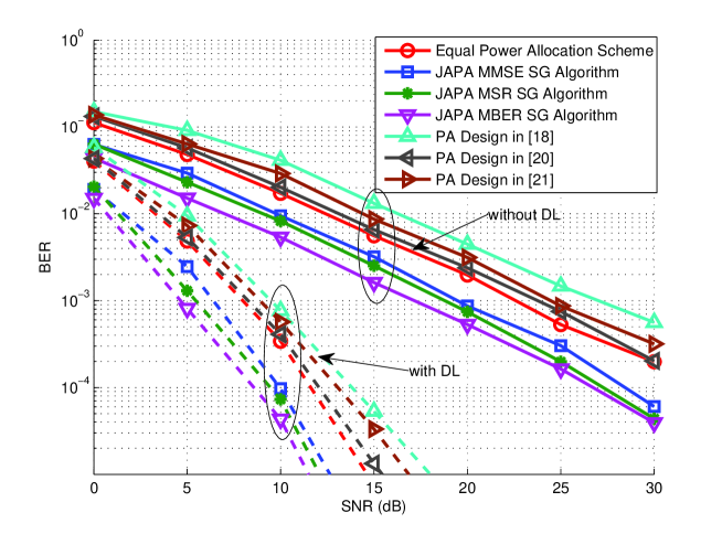
Figure 2: SNR versus BER for JAPA SG Algorithms

The proposed JAPA SG algorithms derived in Section IV are compared with the EPA algorithm and the power allocation algorithms in [21], [23] and [24] with and without the direct link (DL) in Fig. 2. The results illustrate that the performance of the proposed JAPA SG algorithms is superior to the EPA algorithm by more than $3$dB. The performance of the power allocation algorithms in the literature are designed for AF systems without re-encoding at the relays and in order to obtain a fair comparison, they have been adapted to the system considered in Fig. 1. However, as shown in the plot, the performance of the existing power allocation algorithms cannot achieve a BER performance as good as the proposed algorithms. In the low SNR scenario, the JAPA MSR SG algorithm can achieve a better BER performance compared with the JAPA MMSE SG algorithm, while with the increase of the SNR, the BER curves of the JAPA MSR and MMSE SG algorithms approach the BER performance of the JAPA MBER SG algorithm with enough Monte-Carlo simulation numbers. The BER of the JAPA MBER SG algorithm achieves the best performance because of the received BER is minimized by the algorithm in Section IV. The performance improvement of the proposed JAPA SG algorithms is achieved with more relays employed in the system as an increased spatial diversity is provided by the relays.

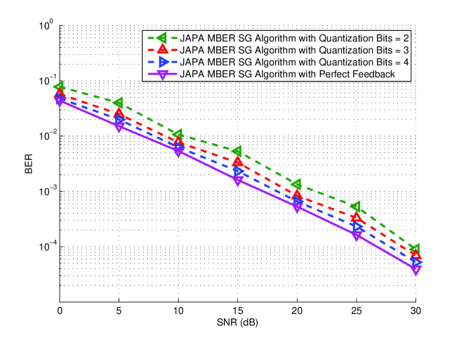
Figure 3: JAPA MBER SG Algorithm SNR versus BER

The simulation results shown in Fig. 3 illustrate the influence of the feedback channel on the JAPA MBER SG algorithm. As mentioned in Section V, the optimized power allocation matrices will be sent back to each relay node and the source node through an AWGN feedback channel. The quantization and feedback errors are not considered in the simulation results in Fig. 2, so the optimized power allocation matrices are perfectly known at the relay node and the source node after the JAPA SG algorithm; while in Fig. 3, it indicates that the performance of the proposed algorithm will be affected by the accuracy of the feedback information. In the simulation, we use $2,~{}3,~{}4$ bits to quantize the real part and the imaginary part of the element in ${\boldsymbol{A}}_{S}[i]$ and ${\boldsymbol{A}}_{k}[i]$, and the feedback channel is modeled as an AWGN channel. As we can see from Fig. 3, by increasing the number of quantization bits for the feedback, the BER performance approaches the performance with perfect feedback, and by making use of $4$ quantization bits for the real and imaginary part of each parameter in the matrices, the performance of the JAPA SG algorithm is about 1dB worse.

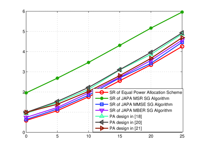
Figure 4: JAPA SG Algorithms Sum Rate versus SNR

The transmission rate of the cooperative MIMO network with EPA and PA schemes in [21], [23] and [24] and the proposed JAPA SG algorithms in Section IV-C is given by Fig. 4. The number of relay nodes is equal to $1$ for all the algorithms. The proposed JAPA MSR SG optimization algorithm adjusts the power allocated to each antenna in order to achieve the maximum of the sum rate in the system. From the simulation results, it is obvious that a higher throughput can be achieved by the existing PA algorithms in [21], [23] and [24] compared to the proposed JAPA MMSE and MBER SG algorithms. The reason for that lies in the design criterion of the existing and the proposed algorithms. However, the improvement in the sum rate by employing the JAPA MSR SG algorithm can be observed as well. The rate improvement of the JAPA MMSE and MBER SG algorithms is not as much as the JAPA MSR SG algorithm because the optimization of the proposed JAPA MMSE and MBER optimization algorithms are not suitable for the maximization of the sum rate.

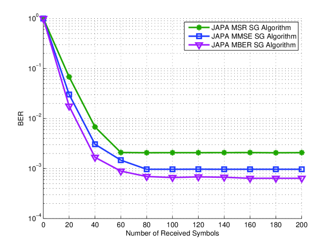
Figure 5: BER performance vs. Number of Symbols for JAPA SG Algorithms

The simulation results shown in Fig. 5 illustrate the convergence property of the proposed JAPA SG algorithm. All the schemes have an error probability of $0.5$ at the beginning, and after the first $20$ symbols are received and detected, the JAPA MMSE scheme achieves a better BER performance compared with the JAPA MSR scheme and the JAPA MBER scheme a better BER than the other algorithms. With the number of received symbols increasing, the BER curve of all the schemes are almost straight, while the BER performance of the JAPA MBER algorithm can be further improved and obtain a fast convergence after receiving $80$ symbols.

VII Conclusion

We have proposed joint adaptive power allocation and receiver design algorithms according to different criteria with the power constraint between the source node and the relay nodes, and between relay nodes and the destination node to achieve low BER performance. Joint iterative estimation algorithms with low computational complexity for computing the power allocation parameters and the linear receive filter have been derived. The simulation results illustrated the advantage of the proposed power allocation algorithms by comparing it with the equal power allocation algorithm. The proposed algorithm can be utilized with different DSTC schemes and a variety of detectors [27] [28] and estimation algorithms [29] in cooperative MIMO systems with AF strategy and can also be extended to the DF cooperation protocols.

References

• [1] P. Clarke and R. C. de Lamare, ”Joint transmit diversity optimization and relay selection for multi-relay cooperative MIMO systems using discrete stochastic algorithms,” IEEE Commun. Lett., vol. 15, pp. 1035-1037, Oct. 2011.
• [2] J. N. Laneman and G. W. Wornell, ”Cooperative diversity in wireless networks: efficient protocols and outage behaviour,” IEEE Trans. Inf. Theory, vol. 50, no. 12, pp. 3062-3080, Dec. 2004.
• [3] P. Clarke and R. C. de Lamare, ”Joint iterative power allocation and relay selection for cooperative MIMO systems using discrete stochastic algorithms,” 8th International Symposium on Wireless Communication Systems (ISWCS), pp. 432-436, Nov. 2011.
• [4] P. Clarke ad R. C. de Lamare, ”Transmit Diversity and Relay Selection Algorithms for Multi-relay Cooperative MIMO Systems”, IEEE Transactions on Vehicular Technology, vol. 61 , no. 3, pp. 1084 - 1098, March 2012.
• [5] T. Peng, R. C. de Lamare and A. Schmeink, “Adaptive Distributed Space-Time Coding Based on Adjustable Code Matrices for Cooperative MIMO Relaying Systems,” IEEE Transactions on Communications, vol.61, no.7, pp.2692-2703, July 2013.
• [6] O. Seong-Jun, D. Zhang and K. M. Wasserman, ”Optimal resource allocation in multiservice CDMA networks,” IEEE Trans. on Wireless Commun., vol. 2, no. 4, pp. 811-821, Jul. 2003.
• [7] A. Khabbazi and S. Nader-Esfahani, ”Power allocation in an amplify-and-forward cooperative network for outage probability minimization,” in 2008 International Symposium on Telecomms., 27-28 Aug. 2008.
• [8] R. C. de Lamare and R. Sampaio-Neto, “Blind adaptive MIMO receivers for space-time block-coded DS-CDMA systems in multipath channels using the constant modulus criterion,” IEEE Transactions on Communications, vol.58, no.1, pp.21-27, January 2010.
• [9] G. Farhadi and N. C. Beaulieu, ”A decentralized power allocation scheme for amplify-and-forward multi-hop relaying systems,” in 2010 IEEE International Conference Communications (ICC), May 2010.
• [10] T. Peng, R. C. de Lamare and A. Schmeink, ”Joint power allocation and receiver design for distributed space-time coded cooperative MIMO systems,” in 2011 8th International Symposium on Wireless Communication Systems (ISWCS), pp. 427-431, 6-9 Nov. 2011.
• [11] T. Peng, R. C. de Lamare and A. Schmeink, ”Joint minimum BER power allocation and receiver design for distributed space-time coded cooperative MIMO systems,” 2012 International ITG Workshop on Smart Antennas (WSA), pp. 225-229, 7-8 March 2012.
• [12] M. Chen, S. Serbetli and A. Yener, ”Distributed power allocation strategies for parallel relay networks,” IEEE Trans. on Wireless Commun., vol. 7, no. 2, pp. 552-561, Feb. 2008.
• [13] J. Luo, R. S. Blum, L. J. Cimini, L. J. Greenstein and A. M. Haimovich, ”Decode-and-forward cooperative diversity with power allocation in wireless networks,” IEEE Trans. on Wireless Commun., pp. 793-799, 2007.
• [14] Y. Jing and B. Hassibi, ”Distributed space-time coding in wireless relay networks,” IEEE Trans. on Wireless Commun., vol. 5, no. 12, Dec. 2006.
• [15] S. Haykin, Adaptive Filter Theory, $4th$ ed. Englewood Cliffs, NJ: Prentice- Hall, 2002.
• [16] A. W. Bowman and A. Azzalini, Applied Smoothing Techniques for Data Analysis, Oxford University Press, Oxford, 1997.
• [17] R.C. de Lamare, R. Sampaio-Neto, “Adaptive MBER decision feedback multiuser receivers in frequency selective fading channels”, IEEE Communications Letters, vol. 7, no. 2, Feb. 2003, pp. 73 - 75.
• [18] S. Chen, A. Wolfgang, Y. Shi, and L. Hanzo, ”Space-time decision feedback equalisation using a minimum bit error rate design for single-input multiple-output channels,” IET Commun., vol. 1, pp. 671-678, August 2007.
• [19] T. Wang, R. C. de Lamare and A. Schmeink, ”Joint linear receiver design and power allocation using alternating optimization algorithms for wireless sensor networks,” IEEE Trans. on Vehi. Tech., vol. 61, pp. 4129-4141, 2012.
• [20] U. Niesen, D. Shah and G. W. Wornell, ”Adaptive alternating minimization algorithms,” IEEE Trans. on Inf. Theory, vol. 55, pp. 1423 - 1429, March 2009.
• [21] J. Liu, N. B. Shroff and H. D. Sherali, ”Optimal power allocation in multi-relay MIMO cooperative networks: theory and algorithms,” IEEE Journal on Selected Areas in Commun., vol. 30, pp. 331-340, February 2012.
• [22] Z. Zhou and B. Vucetic, ”A cooperative beamforming scheme in MIMO relay broadcast channels,” IEEE Trans. on Wireless Commun., vol. 10, pp. 940-947, March 2011.
• [23] W. Guan, H. Luo and W. Chen, ”Linear Relaying Scheme for MIMO Relay System With QoS Requirements,” IEEE Signal Processing Letters, vol. 15, pp. 697-700, December 2008.
• [24] O. Munoz-Medina, J. Vidal and A. Agustin, ”Linear Transceiver Design in Nonregenerative Relays With Channel State Information”, IEEE Trans. on Signal Processing, vol. 55, pp. 2593-2604, May 2007.
• [25] T. Wang, R. C. de Lamare, P. D. Mitchell, “Low-Complexity Set-Membership Channel Estimation for Cooperative Wireless Sensor Networks,” IEEE Transactions on Vehicular Technology, vol.60, no.6, pp. 2594-2607, July 2011.
• [26] K. Zu and R. C. de Lamare, ”Lattice reduction-aided regularized block diagonalization for multiuser MIMO systems,” 2012 IEEE Wireless Communications and Networking Conference(WCNC), pp. 131-135, 1st-4th April 2012.
• [27] H. Vikalo, B. Hassibi, and T. Kailath, ”Iterative decoding for MIMO channels via modified sphere decoding,” IEEE Trans. Wireless Commun., vol. 3, pp. 2299-2311, Nov. 2004.
• [28] R. C. de Lamare and R. Sampaio-Neto, ”Minimum mean-squared error iterative successive parallel arbitrated decision feedback detectors for DS-CDMA systems,” IEEE Trans. on Commun., vol. 56, no. 5, pp. 778 - 789, May 2008.
• [29] R. C. de Lamare and R. Sampaio-Neto, ”Adaptive reduced-rank processing based on joint and iterative interpolation, decimation, and filtering,” IEEE Transactions on Signal Processing, vol. 57, no. 7, pp. 2503 - 2514, July 2009.
• [30] A. Gersho and R. M. Gray, Vector Quantization and Signal Compression, Kluwer Academic Press/Springer, 1992.
• [31] R. C. de Lamare and A. Alcaim, ”Strategies to improve the performance of very low bit rate speech coders and application to a 1.2 kb/s codec” IEE Proceedings- Vision, image and signal processing, vol. 152, no. 1, February, 2005.
• [32] J. H. Choi, H. Y. Yu, Y. H. Lee, “Adaptive MIMO decision feedback equalization for receivers with time-varying channels”, IEEE Trans. Signal Processing, 2005, 53, no. 11, pp. 4295-4303
• [33] C. Windpassinger, L. Lampe, R.F.H. Fischer, T.A Hehn, “A performance study of MIMO detectors,” IEEE Transactions on Wireless Communications, vol. 5, no. 8, August 2006, pp. 2004-2008.
• [34] R.C. de Lamare and R. Sampaio-Neto, “Adaptive Reduced-Rank Equalization Algorithms Based on Alternating Optimization Design Techniques for MIMO Systems,” IEEE Trans. Vehicular Technology, vol. 60, no. 6, pp.2482-2494, July 2011.