Construction of the edge states in fractional quantum Hall systems by Jack polynomial

Abstract

We study the edge-mode excitations of a fractional quantum Hall droplet by expressing the edge state wavefunctions as linear combinations of Jack polynomials with a negative parameter. We show that the exact diagonalization within subspace of Jack polynomials can be used to generate the chiral edge-mode excitation spectrum in the Laughlin phase and the Moore-Read phase with realistic Coulomb interaction. The truncation technique for the edge excitations simplifies the procedure to extract reliably the edge-mode velocities, which avoids the otherwise complicated analysis of the full spectrum that contains both edge and bulk excitations. Generalization to the Read-Rezayi state is also discussed.

I Introduction

The fractional quantum Hall (FQH) effect offers us a unique arena to study strongly correlated electron systems with a collection of effective tools, including many-body model wavefunction, Laughlin (1983) exact diagonalization (successful in often surprisingly small systems), the composite-fermion theory, Jain (2007) conformal field theories (CFT), and Jack polynomials (or Jacks). Bernevig and Haldane (2008a) Of particular interest of these bulk-gapped topological phases of matter are gapless edge excitations, which lead to experimentally measurable charge Chang (2003); Radu et al. (2008) and neutral currents, Bid et al. (2010) including highly nontrivial signals in quasiparticle interference measurement. Willett et al. (2009, 2010, a)

Not only are edge excitations key to transport experiments, they also manifest along artificially cut internal boundary in quantum entanglement studies, clearly demonstrated in the entanglement spectrum Li and Haldane (2008) of FQH systems. The multiplicities in the low-lying part of the entanglement spectrum matches identically with those of the edge excitations with the corresponding boundary conditions. In fact the entanglement spectrum in the case of a real-space cut Dubail et al. (2012a); Sterdyniak et al. (2012); Rodríguez et al. (2012) can be generated by a local field theory along the cut. Dubail et al. (2012b); Kitaev and Preskill (2006)

Explicitly in the disk geometry the model wavefunctions of edge excitations can be obtained by multiplying the corresponding ground-state wavefunction by symmetric polynomials. Wen (1992); Milovanović and Read (1996) The Hilbert space of the edge excitations is robust even in microscopic systems in the presence of long-range interaction, when their excitation energies are comparable to those of bulk excitations. Wan et al. (2003, 2008) In the CFT construction edge states can be expressed as the correlators of bulk CFT primary fields and additional edge fields in the generated chiral algebra. Dubail et al. (2012b) In the Laughlin case, the edge-state Hilbert space can also be generated by a composite-fermion approach. Jolad et al. (2010)

Alternatively, Jack polynomials emerged as one of the effective tools for ground state wavefunction construction. Bernevig and Haldane (2008b); Bernevig and Haldane (2008c); Bernevig and Regnault (2009) Jacks are homogeneous symmetric polynomials and Jacks with negative parameter are shown to be the correlator of the $\mathcal{W}\text{A}_{k-1}(k+1,k+r)$ Feigin et al. (2002, 2003); Estienne and Santachiara (2009) conformal field theory, which includes the $Z_{k}$ parafermion theory. One advantage of using Jack polynomials is that a recursive construction algorithm exists, which renders the exact diagonalization of model Hamiltonians obsolete for a large class of FQH model wavefunctions. Bernevig and Regnault (2009) The Jack polynomials with a negative rational Jack parameter $\alpha$ generate ground-state wavefunctions as well as quasihole wavefunctions, Yang et al. (2012) whose constructions differ only in the corresponding root configurations. By the bulk and edge correspondance in the FQH systems, this implies that one can use Jack polynomials to span the space of FQH states on a disk geometry with single or multiple edge excitations, although they are generically not orthogonal.

The importance of the inner products of edge states in the CFT construction has been emphasized in the context of real-space entanglement spectrum of model FQH states. Dubail et al. (2012b) In particular, these inner products take universal values in the thermodynamic limit, reflecting a correspondance of the edge CFT and the bulk CFT under generalized screening.

In this paper we present a framework to study edge excitations using Jack polynomials, whose coefficients are integers and can be conveniently generated in a computer recursively. Bernevig and Regnault (2009) The main purpose of this paper is to show that an edge state wavefunction, expressed as the corresponding ground state wavefunction (a Jack polynomial itself) multiplied by a symmetric polynomial, can be written alternatively as a linear combination of several Jacks in the corresponding momentum subspace. There is a linear map between the edge-state Hilbert space and the set of admissible root configurations for Jacks with the proper Jack parameter. In fact, the coefficients of the linear combination are universal for all system sizes. By using Jack polynomial to span the edge-state space, we can facilitate numerical calculations involving edge states in the presence of realistic interaction and confinement. Our paper is organized as follows. In section II we review general properties of FQH wavefunctions and basic ingredients of the Jack polynomial approach of the FQH wavefunctions. We discuss the framework for constructing the edge Hilbert space by Jack polynomials in Sec. III. In section IV we apply the approach to generate the edge spectrum for FQH systems in both the Laughlin and the Moore-Read phases with realistic long-range Coulomb interaction by exact diagonalization in the edge-excitation space. Finally, in section V, we summary the paper and discuss potential applications of the framework. In Appendices, we provide the details on several crucial statements in the main text on the Jack polynomial construction of the edge-state Hilbert space.

II FQH wavefunctions and Jack polynomials

II.1 Basic notations

The wavefunction of a free particle in the lowest Landau level (LLL) with the symmetric gauge in a plane is given by

$$\phi_{m}(z)=\frac{1}{\sqrt{2\pi 2^{m}m!}}z^{m}e^{-z\bar{z}/4},\qquad z=x+iy$$ (1)

where $m$ is a non-negative integer representing the angular momentum. Since the Gaussian factor is the same for all $m$, we neglect it in later discussions and only pay attention to polynomials of $z$. It is obvious from the single-particle wavefunction that a many-particle wavefunction must be a multivariate complex polynomial. Depending on the statistics of the particles, the polynomial for the corresponding interacting system is either antisymmetric (for fermions) or symmetric (for bosons). Since a bosonic wavefunction can be mapped to a fermionic wavefunction by the multiplication of a Vandermonde determinant, the discussion hereafter on bosonic wavefunctions (unless we specify otherwise) is sufficient for our purposes.

Since symmetric polynomials form a vector space, one needs to choose a basis. For the description of bosonic wavefunctions by symmetric polynomials the basis of symmetrized monomial (from now on monomial implicitly means symmetrized monomial) is the natural choice; a monomial is nothing but an unnormalized wavefunction for a free particle in the LLL. We will denote a monomial by a sequence of integers, which label the occupied orbitals. For instance, $\boldsymbol{m}_{\{4,2,2,1\}}\equiv\text{Sym}\left(z_{1}^{4}z_{2}^{2}z_{3}^{2}z_{4}^{1}\right)$. In the presence of the rotational symmetry, a many-particle wavefunction has a well-defined total angular momentum $M$. So we only discuss homogeneous symmetric polynomials, whose basis monomials have the same total degree or total angular momentum. It means that the sequence of integers that represents a symmetrized monomial is actually a partition of the total degree (an integer), i.e., a non-increasing sequence of nonzero positive integers whose sum is the integer degree. In the above example $\{4,2,2,1\}$ is a partition of $9$; in other words, it represents a monomial with total angular momentum $9$: one particle in the $z^{4}$ orbital, two in the $z^{2}$ orbital, and the other one in the $z^{1}$ orbital. Normally, the number of particles in the $z^{0}$ orbital is not specified, but its occupation is not ambiguous once the total number of particles is fixed so we can assume that the unspecified particles are in the $z^{0}$ orbital. We denote the weight (the sum of the elements) of a partition $\lambda\equiv\{\lambda_{1},\lambda_{2},\cdots,\lambda_{n}\}$ as $\left|\lambda\right|=\sum_{i=1}^{n}\lambda_{i}$, or the total degree of its representative monomial.

Sometimes, it is more convenient to use the occupation representation (or configuration) to represent a basis. The representations of partition and configuration are of course equivalent, but, just for the sake of convenience and clarity in discussion, we use both representations interchangeably. For instance, the following three notations are considered to be equivalent: $\ket{N-4,1,2,0,1}$, $\{4,2,2,1\}$, and $\boldsymbol{m}_{\{4,2,2,1\}}$, where $N\geq 5$ is the total number of particles. Note that we use the curly bracket for the partition representation and the ket notation for the configuration representation, respectively. Note that the sequence of integers in a configuration specify the corresponding numbers of particles in the orbitals $z^{0},z^{1},z^{2},z^{3},z^{4},\cdots$, respectively.

One can order distinct partitions of an integer by the lexicographical order, but in the context of quantum Hall wavefunctions the dominance order is more convenient. The dominance order is determined by comparing the partial sums of two partitions. Consider two partition $\lambda$ and $\mu$. If $\sum_{i=1}^{j}\lambda_{i}\geq\sum_{i=1}^{j}\mu_{i}$ for every $j$, $\mu$ is dominated by $\lambda$; the relation is denoted by $\mu\preceq\lambda$. In particular, when $\mu$ and $\lambda$ are different, we say $\mu$ is strictly dominated by $\lambda$, or $\mu\prec\lambda$. Dominance is transitive, i.e., if $\nu\preceq\mu$ and $\mu\preceq\lambda$, then $\nu\preceq\lambda$. The dominance ordering only renders a partial order to the whole set of partitions of an integer and admits the lexicographical ordering (i.e., if $\mu\prec\lambda$, $\lambda$ is larger than $\mu$ in lexicographical order).

One can define an instructive operation called squeezing on a partition, which is closely related to the dominance ordering. A squeezing on a partition moves one pair of particles in the angular-momentum space closer $\{\cdots,p,\cdots,q,\cdots\}\to\{\cdots,p-\delta m,\cdots,q+\delta m,\cdots\}$ (reordering can be done afterward to make it a partition). Obviously, the total angular momentum does not change after squeezing. We call the original partition a parent and the result a descendant; the parent partition strictly dominates the descendant partition.

Applying all the possible sequence of squeezing to a partition (which one refers to as a root partition) generates partitions dominated by the root partition. All these descendant partitions, together with the root partition, span a Hilbert space (or a symmetric polynomial space) with a fixed total angular momentum. Studies show that the Hilbert spaces of a certain series of root partitions are closely relate to quantum Hall wavefunctions, which can be expressed as a single Jackpolynomial or the linear combination of a finite set of Jack polynomials. This latter will be ellaborated when we introduce Jack polynomial and, in particular, its application to the edge states of FQH systems. For now, let us denote the Hilbert space spanned by all the partitions dominated by a root configuration $\lambda$ (i.e., $\lambda$ and all the partitions constructed from it by repeated squeezing) as $H_{\text{sq}}(\lambda)$.

II.2 A primer on Jack polynomial

Jack polynomials are homogeneous symmetric polynomials specified by a root configuration and a rational parameter. Jacks satisfy a number of differential equations Feigin et al. (2002) and exhibit clustering properties Bernevig and Haldane (2008d); Feigin et al. (2003). Explicitly, a Jack is one of the polynomial solutions of the following Calogero-Sutherland Hamiltonian

$$H_{CS}^{\alpha}(\{z_{i}\})=\sum_{i}\left(z_{i}\partial_{i}\right)^{2}+\frac{1}{\alpha}\sum_{i<j}\frac{z_{i}+z_{j}}{z_{i}-z_{j}}\left(z_{i}\partial_{i}-z_{j}\partial_{j}\right)$$ (2)

where $\alpha$ is a rational parameter and $\partial_{i}\equiv\partial\left/\partial z_{i}\right.$. The definition of a Jack also requires a root configuration (or partition), such that the Jack polynomial of a given root configuration $\lambda$ is defined in the Hilbert space $H_{\text{sq}}(\lambda)$, which is spanned by all the partitions that can be squeezed from $\lambda$. This fact is due to the structure of the Calogero-Sutherland Hamiltonian, which only couples two partitions if one can be squeezed from another. For a given $\alpha$ we can have a number of Jacks by choosing different root configuration. If $\alpha$ is positive we can choose any kind of partition as root partition and these Jacks are all linearly independent. Therefore, for a positive $\alpha$ Jacks form a basis for symmetric polynomial.

A recursive construction algorithm exists for Jacks of a root configuration $\lambda$ and a Jack parameter $\alpha$ Dumitriu et al. (2007); Thomale et al. (2011). Hence one can compute the coefficients of the following monomial expansion of a Jack

$$J_{\lambda}^{\alpha}(\{z\})=\boldsymbol{m}_{\lambda}+\sum_{\mu\prec\lambda}c_{\mu}\boldsymbol{m}_{\mu}$$ (3)

The convention is to fix the coefficient of the root configuration as unity and other coefficients are scaled accordingly. The use of this set of coefficients in subsequent numerical calculations for a given geometry (e.g., disk or sphere) often requires a proper normalization for each monomial.

Some Jacks of a negative $\alpha$ can be directly related to FQH wavefunctions. It was conjectured that Jacks with a negative parameter with proper root configuration are correlators of certain conformal theories Feigin et al. (2002, 2003). Bernevig and Haldane and co-workers further explored the idea extensively and showed that the Jack polynomial approach is an efficient and insightful development to obtain and to exploit FQH wavefunctions Bernevig and Haldane (2008b); Bernevig and Haldane (2008c, d); Bernevig and Haldane (2009); Bernevig and Regnault (2009). It was proven for general $(k,r)$ that Jacks are the correlators of $\mathcal{W}\text{A}_{k-1}(k+1,k+r)$ conformal theories Bernevig et al. (2009); Estienne and Santachiara (2009). In other words, the correlators are eigenfunctions of the Calogero-Sutherland Hamiltonian [Eq. (2)]. Further more, the application of Jack polynomial on a certain type of quasihole wavefunctions was also proposed and proven to be correct with the discovery of interesting duality structure between electron and quasihole wavefunctionsBernevig and Haldane (2008b); Estienne et al. (2010).

In contrast to a positive $\alpha$, we have, for a negative $\alpha$, restrictions on the choice of root configuration. One allowed choice is to use a $(k,r)$ admissible root configuration, which leads to legitimate FQH trial wavefunctions. The $(k,r)$-admissibility means that there can be at most $k$ particles in $r$ consecutive orbitals. More precisely, a partition $\lambda$ is said to be $(k,r)$ admissible, if $\lambda_{i}-\lambda_{i+k}\geq r$. The densest $(k,r)$ admissible root configuration and a corresponding Jack parameter $\alpha=-(k+1)/(r-1)$ (with the condition that $k+1$ and $r-1$ are coprime) generate the FQH ground state with a filling fraction $\nu=k/r$ (corresponding to $\nu=k/(k+r)$ in the fermionic case). Note that $\alpha$ is negative.

$\left(k,r\right)$	bosonic	$\left(k,k+r\right)$	fermionic
$\left(1,2\right)$	$\ket{1,0,1,0,1,\cdots,1}$	$(1,3)$	$\ket{1,0,0,1,0,0,1,\cdots,1}$
$\left(1,4\right)$	$\ket{1,0,0,0,1,\cdots,1}$	$(1,5)$	$\ket{1,0,0,0,0,1,\cdots,1}$
$\left(2,2\right)$	$\ket{2,0,2,0,2,\cdots,2}$	$(2,4)$	$\ket{1,1,0,0,1,1,\cdots,1,1}$

Table 1: The densest $(k,r)$ admissible configurations. Fermionic configuration is $(k,k+r)$ admissible configurations which is the counter part state of $(k,r)$ admissible bosonic configuration.

The applicability of the Jacks to the fermionic case is highly nontrivial since the multiplication of a Jack (with a monomial expansion) with a Vandermonde determinant cannot be straightforwardly mapped to a sum of Slater determinants. Nevertheless, a recursive procedure was found to generate the Slater-determinant expansion of $\prod_{i<j}\left(z_{i}-z_{j}\right)J_{\lambda}^{\alpha}(\{z\})$ Bernevig and Regnault (2009); Thomale et al. (2011). Hence, all the discussion on bosonic wavefunctions, including numerical calculation, is applicable to fermionic wavefunctions in practice.

III Jack polynomials for FQH edge states

III.1 Laughlin edge states: an example

In the simplest case of an Abelian Laughlin state, edge excitations are deformation of edge density of the incompressible liquid. One can write down the trial wavefunction for an edge state as a symmetric polynomial multiplied by the ground state wavefunction Wen (1992)

$$\Psi(\{z\})=S(\{z\})\Psi_{L}^{r}(\{z\})$$ (4)

where $\Psi_{L}^{r}=\prod_{i<j}^{n}\left(z_{i}-z_{j}\right)^{r}$ is the Laughlin state at a filling fraction $\nu=1/r$ (with total angular momentum of $M_{0}=rN(N-1)/2$) and $S(\{z\})$ a homogeneous symmetric polynomial. In this expression we encounter the multiplication of a monomial by another, which is then to be expanded as a sum of monomials. The expansion is not straightforward and often computationally expensive. Similarly, a symmetrized monomial multiplied by a antisymmetric Vandermonde determinant is in general a complex superposition of antisymmetrized monomials (or Slator determinants). The same difficulty also arises in the wavefunctions of quasihole states. Therefore, the nontrivial multiplication of physically natural basis states hinders us to efficiently use ansatz edge-state or quasihole-state wavefunctions in computation. The difficulty, however, can be resolved by the introduction of Jack polynomial Bernevig and Regnault (2009). In this paper, we focus on the applications for the edge-state wavefunctions.

The edge state, as well as the ground state, is a zero-energy eigenstate of an ideal Hamiltonian with short-range interaction. One remarkable fact about Eq. (4) is that the number of linearly independent edge states for a given momentum ($M=M_{0}+\Delta M$) predicted by the chiral Luttinger liquid theory is the same as the number of the symmetric polynomials of degree $\Delta M$. To see this, it is sufficient to check the dimension of the legitimate symmetric polynomials for the given momentum $M$. By counting the number of possible monomials of degree $\Delta M$ or possible partitions of $\Delta M$, we obtain the dimension of the edge-state subspace with a total angular momentum $M=M_{0}+\Delta M$. Hence the subspace dimension for the given momentum $\Delta M$ is exactly the number of partition of the integer $\Delta M$ and the counting is consistent with the edge theory of a single branch of chiral bosons.

Given the fact that the Laughlin state can be expressed as a single Jack with a root configuration being a $(k,r)$ admissible partition of $M_{0}$, one natually wants to explore the connection of the edge states to Jacks with root configurations being $(k,r)$ admissible partitions of $M>M_{0}$. The clustering property is enforced such that the Jacks are also zero-energy states of the ideal Hamiltonian. In other words, these Jacks are edge states. One immediate question is whether the distinct Jacks span the same edge-state Hilbert space. A harder question is how to relate the edge states, given by Eq. (4), and the Jacks of various root configurations; they are in general not orthorgonal to one another within each group. Because one can form a quasihole wavefunction by a linear combination of edge excitations with proper weight, the construction of edge states by superposing Jack polynomials leads straightforwardly to the construction of quasihole wavefunctions Bernevig and Haldane (2008b); Estienne et al. (2010) in the same manner.

III.2 Edge Jacks polynomials

As we argued above, admissible root configurations with larger angular momentum (than the ground state anngular momentum) lead to Jacks in the Hilbert space of edge states because of the clustering property of the Jacks. But so far we do not know the explicit relation between these Jacks and the ansatz wavefunctions for edge states, which is crucial if one wants to efficiently expand any edge-state wavefunction into monomials.

To explicitly show that the Jacks with $(k,r)$ admissible partitions span the same Hilbert space as the edge states described by Eq. (4), we introduce a compact notation for the admissible root configurations. In this notation the admissible root configuration for an edge state is obtained by adding to the ground state root configuration $\Omega$ a partition $\eta$ of $\Delta M$, or $\lambda=\Omega+\eta$. Note that the total angular momentum of the Jacks wavefunction of $\lambda$ is $\left|\Omega\right|+\left|\eta\right|$, or $M=M_{0}+\Delta M$. Hence, once $(k,r,N)$ is fixed one can label a state only by $\eta$, which we refer later as the edge partition, without any ambiguities. As a concrete example, we consider the Laughlin sequence, for which $k=1$ and $r$ is a certain positive even integer. The $(1,r)$ admissibility of the densest ground state means $\Omega_{i}-\Omega_{i+1}=r$. The difference changes to $\lambda_{i+1}-\lambda_{i}=(\Omega_{i}-\Omega_{i+1})+(\eta_{i}-\eta_{i+1})=r+(\eta_{i}-\eta_{i+1})$, when $\eta$ is added to $\Omega$. Therefore, the $(1,r)$ admissible condition of $\lambda=\Omega+\eta$ is that $\eta$ is a nondecreasing sequence of integers, which precisely means that $\eta$ is a partition of the additional angular momentum $|\eta|=\Delta M$. This identification of $\eta$ gives exactly the expected number of the edge states described by Eq. (4). Note that $\eta$ is meaningful for any system with $N\geq\Delta M$ and, in this case, the number of $(1,r)$ admissible root configurations, hence of linearly independent edge states, are independent of the particle number $N$. The analysis of $(k,r)$ admissible states with $k>1$ needs more care, as $\eta$ cannot be a simple partition. We defer the discussion to Appendix A.

These admissible root partitions themselves are related by squeezing or dominance ordering. Regardless of $(k,r)$, the greatest partition for a given $\Delta M$ is $\lambda_{\Delta M}=\Omega+\{\Delta M\}$ and the other admissible partitions are dominated by it. This implies that the Hilbert space for a Jack with an admissible root partitions is a subspace of $H_{sq}(\lambda_{\Delta M})$. Moreover, $H_{sq}(\lambda_{1})\subset H_{sq}(\lambda_{2})$ if the two partitions satisfy $\lambda_{1}\prec\lambda_{2}$ by dominance ordering. It means that the dominance relation between the root configurations is sufficient to describe the inclusion relation of the Hilbert space for the Jacks generated by the respective root configurations.

Now we consider the concrete construction of the edge-state space for the Laughlin case, i.e. $k=1$. The dominance relation between $\lambda$s is same as the corresponding $\eta$s. Therefore, in lieu of Eq. (4) one may expect a set of equations that relate the Jacks with the edge partition $\eta$s as their roots and the Jacks with the full partition $\lambda$s. Indeed, we find

$$J_{\Omega+\eta}^{\alpha}=J_{\eta}^{\beta}J_{\Omega}^{\alpha}$$ (5)

where $\alpha=-\frac{2}{r-1}$ and $\beta=\frac{2}{r+1}$. We leave the derivation in Appendix B. Note that there is no restriction on the root configuration for the positive rational parameter $\beta$. The result means that $J_{\eta}^{\beta}$ is a representation of $J_{\Omega+\eta}^{\alpha}$ that can be readily used to decompose any edge state in the form of Eq. (4). For an arbitrary symmetric polynomial $S({z})$, one can expand it in terms of Jacks $J_{\eta}^{\beta}$, since the Jacks form a basis for the homogeneous symmetric polynomial space. Therefore, it is possible to obtain the monomial expansion of $S({z})J_{\Omega}^{\alpha}$ efficiently.

As an important example, we consider the monomial expansion of an arbitrary monomial multiplied by the Laughlin ground state $J_{\Omega}^{\alpha}$ for $\alpha=-2/(r-1)$. In other words, we want to calculate the coefficient $c_{\mu}$ in the expression

$$\boldsymbol{m}_{\eta}J_{\Omega}^{\alpha}=\sum_{\mu\preceq\Omega+\eta}c_{\mu}\boldsymbol{m}_{\mu}.$$ (6)

This can be easily achieved once we know the monomial expansion of $J_{\eta}^{\beta}$. By inverting the relation between $\boldsymbol{m}_{\eta}$s and $J_{\eta}^{\beta}$s, one can express any $\boldsymbol{m}_{\eta}$ as a linear combination of $J_{\eta}^{\beta}$s. In other words, one then obtains a Jack-polynomial expansion of the monomial multiplied by the ground state wavefunction. We can, equivalently, write down the array of equations in a compact form for any $\Delta M$ as

$$\mathbf{J}\mathbf{m}J_{\Omega}^{\alpha}=\mathbf{j}_{E},$$ (7)

where $\mathbf{j}_{E}$ is a column vector whose components are the edge Jacks $J^{\alpha}_{\Omega+\eta}$ and $\mathbf{m}$ a vector of $\boldsymbol{m}_{\eta}$s; both are ordered in the lexicographical order of $\eta$. Explicitly, we have

$$\mathbf{j}_{E} = \left(J^{\alpha}_{\Omega+\{1,\cdots,1\}},\cdots,J^{\alpha}_{\Omega+\{\Delta M\}}\right)^{T},$$ (8)

$$\mathbf{m} = \left(\mathbf{m}_{\{1,\cdots,1\}},\cdots,\mathbf{m}_{\{\Delta M\}}\right)^{T}.$$ (9)

They have the same dimension, which is the number of all possible partitions of $\Delta M$. $\mathbf{J}$ is a matrix, which consists of the corresponding coefficients of $J_{\eta}^{\beta}$ in terms of $\boldsymbol{m}_{\nu}$, i.e.,

$$\mathbf{J}_{\eta\nu}=c^{(\eta)}_{\nu},$$ (10)

if we assume

$$J^{\beta}_{\eta}=\sum_{\nu\preceq\eta}c^{(\eta)}_{\nu}\mathbf{m}_{\nu}.$$ (11)

Again, we recall the convention $c^{(\eta)}_{\eta}=1$. By inverting $\mathbf{J}$, we obtain

$$\mathbf{m}J_{\Omega}^{\alpha}=\mathbf{J}^{-1}\mathbf{j}_{E}.$$ (12)

Since the rank of $\mathbf{J}$ is only the number of distinct partitions of $\Delta M$, the computation of $\mathbf{J}$ and its inverse is computationally cheap.

We point out two important properties of $\mathbf{J}$ in the following. Firstly, when we arrange the basis (for both the Jacks by their root partitions and the monomials) in lexicographical order or any other order that respects the dominance ordering, we obtain a lower triangular matrix with all identities at its diagonal (i.e., a unitriangular matrix) for $\mathbf{J}$. In other words, if $\mu>\lambda$ by dominance ordering or has no relation between $\mu J_{\Omega}^{\alpha}$ and $\lambda$, then the inner product of $\mathbf{m}_{\mu}$ and $J_{\lambda}$ is zero, as the two share no common monomials in their respective expansions. We note that $H_{sq}(\Omega)H_{sq}(\eta)\subset H_{sq}(\Omega+\eta)$ for our understanding, which can be proved as in Appendix C and which indicates that $\mathbf{m}_{\eta}J_{\Omega}^{\alpha}\subset H_{sq}(\Omega+\eta)$. Secondly, as long as the number of particles is larger than $\Delta M$, $\mathbf{J}$ is independent of system size. As an example, let us define $\eta_{1}=\{1,1,1,1\}$, $\eta_{2}=\{2,1,1\}$, $\eta_{3}=\{2,2\}$, $\eta_{4}=\{3,1\}$, and $\eta_{5}=\{4\}$ for $k=1$, $r=2$, and $\Delta M=4$. We have

$$\left(\begin{array}[]{c}\mathbf{m}_{\eta_{1}}\\ \mathbf{m}_{\eta_{2}}\\ \mathbf{m}_{\eta_{3}}\\ \mathbf{m}_{\eta_{4}}\\ \mathbf{m}_{\eta_{5}}\end{array}\right)J_{\Omega}^{\alpha}=\left(\begin{array}[]{ccccc}1&0&0&0&0\\ -\frac{36}{11}&1&0&0&0\\ \frac{27}{22}&-\frac{6}{5}&1&0&0\\ \frac{27}{11}&-\frac{27}{25}&-\frac{6}{5}&1&0\\ -\frac{81}{55}&\frac{36}{25}&\frac{6}{35}&-\frac{4}{3}&1\end{array}\right)\left(\begin{array}[]{c}J^{\alpha}_{\Omega+\eta_{1}}\\ J^{\alpha}_{\Omega+\eta_{2}}\\ J^{\alpha}_{\Omega+\eta_{3}}\\ J^{\alpha}_{\Omega+\eta_{4}}\\ J^{\alpha}_{\Omega+\eta_{5}}\end{array}\right)$$ (13)

where the matrix on right hand side is $\mathbf{J}^{-1}$, the inverse of

$$\mathbf{J}=\left(\begin{array}[]{ccccc}1&0&0&0&0\\ \frac{36}{11}&1&0&0&0\\ \frac{27}{10}&\frac{6}{5}&1&0&0\\ \frac{108}{25}&\frac{63}{25}&\frac{6}{5}&1&0\\ \frac{72}{35}&\frac{12}{7}&\frac{10}{7}&\frac{4}{3}&1\end{array}\right)$$ (14)

The electron number independence of $\mathbf{J}$ is guaranteed by product rule Bernevig and Regnault (2009); Thomale et al. (2011) of Jacks. If the electron number $N$ is larger than $\Delta M$, then the admissible root partitions are in one-to-one correspondance with those of the system with $N=\Delta M$. Hence by the product rule, the coefficients of the admissible root partitions remain unchanged with increasing system size.

Before we move on to the more general cases (i.e., $k>1$), we emphasize that the form of $\mathbf{J}$ for $k=1$ is the direct consequence of Eq. (5). We do not know any such simple relation for $k>1$, hence the form of $\mathbf{J}$ is not as simple but still can be computed. The reason for the complication is because an edge sequence is no longer a simple partition, but consists of $k$ subpartitions. However, the Jacks with admissible root configurations still exhaust the Hilbert space of the edge states, therefore, we can still expand any edge-state wavefunction as a linear combinations of the edge Jack polynomials. That is to say, we look for a generalization of Eq. (7) or Eq. (12). As the edge space is no longer spanned by simple monomials multiplied by the ground state. Nevertheless, we can still write down a complete set of edge states for each $\Delta M$ (which we label as $\mathbf{m}_{E}$ that replaces ${\mathbf{m}}J_{\Omega}^{\alpha}$), as Milovanović and Read did for the $k=2$ Moore-Read case. Now the question converts to how to create a dictionary $\mathbf{J}$ to translate $\mathbf{m}_{E}$, which is normally easier for analytical discussions, to the set of edge Jack polynomials $\mathbf{j}_{E}$, which is more convenient for numerical calculations. Note that, in the basis of monomials of degree $M_{0}+\Delta M$ [i.e. in the Hilbert space $H_{sq}(\Omega+\{\Delta M\})$], $\mathbf{m}_{E}$ and $\mathbf{j}_{E}$ can be viewed, alternatively, as matrices. A key observation is that the dimension of edge state (number of rows) is usually much smaller than the dimension of $H_{sq}(\Omega+\{\Delta M\})$ (number of columns), such that we do not need to know all elements of $\mathbf{m}_{E}$ to obtain $\mathbf{J}$; in other words, we have a set of overdetermined linear equations. The most obvious solution to the problem which subspace in $H_{sq}(\Omega+\{\Delta M\})$, whose dimension is the same as that of the edge space, should be chosen to determine $\mathbf{J}$ turns out to be the space spanned by admissible root partitions.

This can be further extended to express, in terms of Jacks, quasihole states (including multiple quasiholes), which can be written as the superpositions of edge states with powers of the quasihole coordinates as coefficient and which we will not elaborate.

IV Numerical applications

IV.1 Diagonalization in the truncated space of edge states

One of the applications of the edge Jacks is the exact diagonalization of the Hamiltonian with realistic Coulomb interaction within the edge-state subspace spanned by the Jacks. The exact diagonalization in the full Hilbert space is difficult bacause of its exponentially growing size as particle number increases. Fortunately, the low-energy eigenfunctions of the Hamiltonian are well represented by CFT correlators or Jacks so we can overcome this difficulty by projecting the Hamiltonian to the edge-state subspace. For electrons we use the fermionic Jacks, which are symmetric Jacks multiplied by a Vandermonde determinant. The recursive construction procedure is well documented in Ref.Bernevig and Regnault, 2009. Here we consider a realistic Hamiltonian

$$H=\frac{1}{2}\sum_{mnl}V^{l}_{mn}c_{m+l}^{\dagger}c_{n}^{\dagger}c_{n+l}c_{m}+\sum_{m}U_{m}c_{m}^{\dagger}c_{m},$$ (15)

where the Coulomb matrix elements $V^{l}_{mn}$ are

$$V^{l}_{mn}=\int d^{2}r_{1}\int d^{2}r_{2}\phi_{m+l}^{*}(\vec{r}_{1})\phi_{n}^{*}(\vec{r}_{2})\frac{{e^{2}}}{{\varepsilon r_{12}}}\phi_{n+l}(\vec{r}_{1})\phi_{m}(\vec{r}_{2}),$$ (16)

and $U_{m}$ is the matrix element of the rotationally invariant confining potential due to the disk-shaped positive background charge at a setback distance $d$

$$U_{m}={N_{e}e^{2}\over\pi R^{2}\varepsilon}\int d^{2}r\int_{\rho<R}d^{2}\rho\frac{|\phi_{m}(\vec{r})|^{2}}{\sqrt{|\vec{r}-\vec{\rho}|^{2}+d^{2}}}.$$ (17)

Here $\varepsilon$ is the dielectric constant and $R$ the radius of the background charge disc.

The diagonalization can be performed in the subspace of Jacks with a fixed momentum due to the rotational invariance. For instance, for $\Delta M=3$, available $\eta$s of Laughlin sequence are $\{3\}$,$\{2,1\}$ and $\{1,1,1\}$. Hence the subspace we deal with are only $3$ dimension consists in $J_{\Omega+\{3\}},J_{\Omega+\{2,1\}}$ and $J_{\Omega+\{1,1,1\}}$. Since Jacks are not orthogonal to each other, orthogonalization is needed. We project the Hamiltonian to the subspace spanned by the orthogonalized edge basis and then perform the exact diagonalization. The result for 9 electrons at $d=0.6l_{B}$ is shown in Fig.1(a). The low-lying spectrum is in good agreement with that from the exact diagonalization in the full Hilbert space. A similar comparison for the Moore-Read phase with 12 electrons are shown in Fig.1(b) and (c). We illustrate here, as in Ref. Wan et al., 2008, the diagonalization results for a mixed Hamiltonian with both Coulomb and three-body interaction, i.e., $H=(1-\lambda)H_{\text{Coulomb}}+\lambda H_{3B}$. Explicitly, the three-body interaction $H_{3B}$, which generates the Moore-Read wavefunction as its exact ground state, has the form

$$H_{3B}=-\sum_{i<j<k}S_{ijk}[\nabla^{2}_{i}\nabla^{2}_{j}(\nabla^{2}_{i}+\nabla^{2}_{j})\delta({\bf r}_{i}-{\bf r}_{j})\delta({\bf r}_{i}-{\bf r}_{k})],$$ (18)

where $S$ is a symmetrizer: $S_{123}[f_{123}]=f_{123}+f_{231}+f_{312}$, where $f$ is symmetric in its first two indices. When $\lambda=0.5$, the edge states, which are zero-energy states for $H_{3B}$, pick up finite energies but are still well separated from the bulk states in small excitation-momentum sectors. Fig.1(b) shows that the edge-state spectrum agrees well with that from the full diagonalization. In the case of the pure Coulomb interaction in Fig.1(c), the agreement is not as good due to the mixing of the edge states with the bulk states. Wan et al. (2008)

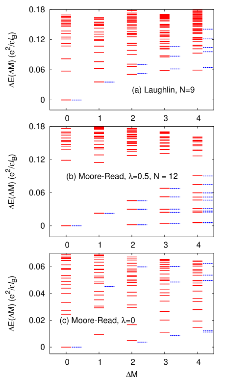
Figure 1: The comparison of the low-energy excitation spectra from the exact diagonalization in the full Hilbert space (red bars) and from the diagonalization within the edge Jack polynomial subspace (blue bars with an artificial shift in momentum for clarity). (a) The Laughlin case with 9 electrons. (b) and (c) are for Moore-Read case with 12 electrons. Here, $\lambda$ is the parameter for the mixed Hamiltonian with three-body interaction $H=(1-\lambda)H_{\text{Coulomb}}+\lambda H_{3B}$, as in Ref. Wan et al., 2008. $\lambda=0$ is the case of pure Coulomb interaction.

From the comparison of the excitation spectra in Fig.1 of the full-space diagonalization and the truncated-space diagonalization we have the following observation. For small excitation-momentum sectors, the energies are almost identical in two cases. Even for $\nu=5/2$ state with the Coulomb interaction, their difference decreases as the system size increases and vanishes in the thermodynamic limit. This is particularly useful to extract the edge velocities, to be discussed in the next subsection, from the truncated-space diagonalization for system sizes significantly larger than those can be handled by the full diagonalization. For regular computing systems, the main bottleneck of this method for large systems is the large storage space (or memory) for the edge Jacks.

IV.2 Edge-Mode Velocities

Edge-mode velocities in the Moore-Read phase and the Read-Reazyi phase are important non-universal quantities, as they are closely related to the decoherence length of the non-Abelian quasiparticles propagating along the edge of, say, a quasiparticle interferometer. Their calculation can be made more efficient with the help of the diagonalization in the space spanned by the edge Jacks. Charge mode velocity can be defined as $v_{b}=L(E_{0}(\Delta M=1)-E_{0}(\Delta M=0))[e^{2}/\epsilon\hbar]$, where the perimeter of the quantum droplet is $L=2\pi R=\sqrt{2N(k+r)/k}$. Neutral mode velocity can be defined as $v_{f}=L(E_{0}(\Delta M=2)-E_{0}(\Delta M=0))/2[e^{2}/\epsilon\hbar]$. Hu et al. (2009) $E_{0}(\Delta M)$ is the lowest eigenenergy for the given momentum $\Delta M$. Through finite-size scaling we can extrapolate the edge-mode velocities in the thermodynamic limit. We have demonstrated the applicability of the finite-size scaling with data from the diagonalization in the full Hilbert space in Ref. Hu et al., 2009.

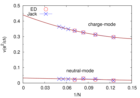
Figure 2: Finite-size scaling of the edge-mode velocities for $\nu=5/2$ with Coulomb interaction and confinement from neutralizing background charge. The charge-mode velocity is fitted by a quadratic function in $1/N$ and, in the thermodynamic limit, the velocity reads $0.44e^{2}/\epsilon\hbar$ (based on data from 8-20 particles). The neutral-mode velocity is fitted by a linear dependence on $1/N$. In the thermodynamic limit, the velocity reads $0.033e^{2}/\epsilon\hbar$.

We first apply the velocity calculation to the 1/2-filling Moore-Read case, i.e. $k=2$ and $r=2$, in the first excited Landau level. With the diagonalization in the edge-state space we can handle systems with up to 20 electrons. Fig. 2 shows that a charge-mode velocity of $0.44e^{2}/\epsilon\hbar$ can be extrapolated in the thermodynamic limit. This value agrees with the previous finite-size scaling result based on the exact diagonalization of systems of 8-14 electrons. Hu et al. (2009). The neutral-mode velocity suffers more from the the finite-size effect due to its smallness and can be extrapolated to be $0.033e^{2}/\epsilon\hbar$ in the thermodynamic limit. We confirm the sharp contrast in the magnitude of the charge-mode and neutral-mode velocities. As discussed in earlier works, Wan et al. (2008); Hu et al. (2009) this sets an upper limit of about 1 $\mu$m for the coherence length for charge-e/4 quasiparticles at 5/2 filling factor in a Fabry-Perot interferometer. Recently, Willett and co-workers Willett et al. (b) reported such coherence length to be 0.49-0.74 $\mu$m, consistent with our study of the edge-mode velocities in the realistic model.

We also attempted the same analysis of edge velocities for the Read-Rezayi state at filling fraction 13/5 with Coulomb interaction, whose particle-hole conjugated state at 12/5 filling has been observed in some experiments Xia et al. (2004); Kumar et al. (2010); Zhang et al. (2012). Preliminary results suggest that, again for $d/l_{B}=0.6$, the charge-mode velocity is $0.537e^{2}/\epsilon\hbar$ (roughly 6/5 times the charge-mode velocity at 5/2 filling as expected) while the neutral-mode velocity is extrapolated to almost zero (more precisely, another order of magnitude smaller than the neutral-mode velocity in the Moore-Read case). The smallness of the neutral-mode velocity is a strong indication that the Read-Rezayi is very fragile in reality. The small value can be very sensitive to Landau level mixing, which remains to be explored. Nevertheless, we expect that the qualitative conclusion that the neutral-mode velocity is much smaller than the charge-mode velocity will still be valid.

V Conclusion

In summary, we discuss the identification of the Hilbert space of edge excitations in the Laughlin–Moore-Read–Read-Rezayi series as spanned by the appropriate Jack polynomials with admissible root configurations. In particular, we elaborate on the Laughlin case ($k=1$), which contains a single charged mode. We explain how to establish a linear map between the polynomial edge wavefunctions and edge Jack polynomials. The map is of particular use in the presence of realistic interaction and confinement, in which case the edge spectrum has a nontrivial dispersion with a nonuniversal edge-mode velocity. The mapping formalism and its numerical application can be generalized to larger $k$s. The applicability has been checked by the comparison of the edge spectra obtained in the truncated edge Jack polynomial space and in the full Hilbert space with exact diagonalization. The truncation approach has the advantage of being able to treat larger systems than the conventional exact diagonalization approach. As an example, we are able to calculate the edge-mode velocities in the Moore-Read phase for $\nu=5/2$ up to 20 electrons and confirm with greater confidence that the neutral-mode velocity is an order of magnitude smaller than the charge-mode velocity.

This work was supported by the 973 Program under Project No. 2012CB927404 and NSFC Projects No. 11174246 and No. 11274403. K.H.L. acknowledges the support at the Asia Pacific Center for Theoretical Physics from the Max Planck Society and the Korea Ministry of Education, Science and Technology.

Appendix A Edge partitions for $k>1$

To discuss $(k,r)$ admissible states with $k>1$ is more complicated, as $\eta$ cannot be a simple partition. To systemically classify these admissible edge states, it is necessary to separate a partition into $k$ sequences. By doing so we get a set of $\eta^{(1)}$, … ,$\eta^{(k)}$, where $\eta^{(i)}$ = $\left\{\eta_{i},\eta_{i+k},\eta_{i+2k},\cdots,\eta_{n-k+i}\right\}$. The $(k,r)$ admissible condition of $\lambda$ implies that

$$\eta^{(i\bmod k)}_{\lceil i/k\rceil}-\eta^{(i\bmod k)}_{\lceil i/k\rceil+1}=\eta_{i}-\eta_{i+k}=(\lambda_{i}-\lambda_{i+k})-r\geq 0$$ (19)

where $\lceil x\rceil$ is the smallest integer greater than or equal to $x$. In other words, $\eta^{(i)}$ is a partition of $\left|\eta^{(i)}\right|$. But unlike the $k=1$ case, not every partition of a given angular momentum is qualified as $\eta^{i}$. If $k\neq 1$ we have two conditions that exist among $\eta^{(i)}_{j}$s. The first condition is that $\eta^{(i)}_{j}\geq\eta^{(i+1)}_{j}$. This condition implies that $|\eta^{(i)}|\geq|\eta^{(i+1)}|$, which is weaker. So, $\{|\eta^{(1)}|,|\eta^{(2)}|,\cdots,|\eta^{(k)}|\}$ is itself a partition of $\Delta M$. The second condition is that $\eta^{(i)}_{j}<\eta^{(i+1)}_{j+1}+r$ for every $1\leq i\leq k$ and $j\geq 1$. Without such conditions, two different $\eta$ can be assign to the same state. For example, the additions of two sets of partitions $\eta^{(1)}=\{2\}$, $\eta^{(2)}=\{1\}$ and $\xi^{(1)}=\{1\}$, $\xi^{(2)}=\{2\}$ generate the same state for the Moore-Read ground state with a densest root configuration $\{2,0,2,\cdots\}$. Careful examination leads to the conclusion that the above two conditions are sufficient to generate a unique representation. These conditions are easily depicted by a Ferres diagram in Fig. 3. The counting of $\eta$ is not as straightforward as in the $k=1$ case, but can be done by partitioning the angular momentum of the edge excitation into $k$ ordered partitions as discussed here. The counting of $(k,2)$ and $(k,3)$ admissible partitions are also considered in Ref. Bernevig and Haldane, 2008c to compute the specific heat of FQH states.

Figure 3: Ferres diagrams for the constraints on the edge partitions for $k=2$ (left) and $k=3$ in the Read-Rezayi series with $r=2$ (right). The left Ferres diagram illustrates how an edge parition is determined for $k=2$. In the example, the edge partition can be bipartited into $\eta^{(1)}=\{7,6,5,5,2\}$ and an $\eta^{(2)}$ to be determined. The subpartition represented by the white cells (including the grey cells) is $\eta^{(1)}$ and partition represented by the grey is a partition obtained by shifting $\eta^{(1)}$ upward by 1 and leftward by $r=2$. As discussed in the text, an allowed $\eta^{(2)}$ should be dominated by $\eta^{(1)}$ but dominate the grey-cell partition. The right Ferres diagram illustrates the case for $k=3$, assuming that $\eta^{(2)}$ is already selected based on the left Ferres diagram, e.g., $\eta^{(2)}=\{4,3,3\}$ (grey and dark grey cells) for the same $\eta^{(1)}=\{7,6,5,5,2\}$ (white, grey, and dark grey cells). $\eta^{(3)}$ should be dominated by $\eta^{(2)}$, but dominate the partition represented by dark grey cells, obtained by shifting $\eta^{(2)}$ upward by 1 and leftward by $r=2$.

Appendix B Derivation of Eq. (5)

To verify the relation $J_{\Omega+\eta}^{\alpha}=J_{\eta}^{\beta}J_{\Omega}^{\alpha}$ where $\alpha=-\frac{2}{r-1}$ and $\beta=\frac{2}{r+1}$ (i.e. $k=1$), we start with the Calogero-Sutherland Hamiltonian $H_{CS}=\sum_{i}z_{i}D_{i}^{L,-1}z_{i}D_{i}^{L,r}$, where $D_{i}^{L,r}=\partial_{i}-r\sum_{j(\neq i)}\frac{1}{z_{i}-z_{j}}$ and, importantly, $D_{i}^{L,r}J_{\Omega}^{\alpha}=0$, Bernevig and Haldane (2008b), and apply it to $J_{\eta}^{\beta}J_{\Omega}^{\alpha}$.

$$\sum_{i}z_{i}D_{i}^{L,-1}z_{i}D_{i}^{L,r}J_{\eta}^{\beta}J_{\Omega}^{\alpha}=\sum_{i}z_{i}D_{i}^{L,-1}z_{i}J_{\Omega}^{\alpha}\partial_{i}J_{\eta}^{\beta}\\ =\sum_{i}\left[z_{i}J_{\Omega}^{\alpha}\partial_{i}J_{\eta}^{\beta}\right.+z_{i}^{2}J_{\Omega}^{\alpha}\partial_{i}^{2}J_{\eta}^{\beta}\\ \left.+z_{i}^{2}\partial_{i}J_{\Omega}^{\alpha}\partial_{i}J_{\eta}^{\beta}+z_{i}^{2}J_{\Omega}^{\alpha}\sum_{j(\neq i)}\frac{\partial_{i}J_{\eta}^{\beta}}{z_{i}-z_{j}}\right]\\ =J_{\Omega}^{\alpha}\left(\sum_{i}\left[z_{i}\partial_{i}J_{\eta}^{\beta}+z_{i}^{2}\partial_{i}^{2}J_{\eta}^{\beta}\right]\right.\\ \left.+(1+r)\sum_{i\neq j}\frac{z_{i}^{2}\partial_{i}J_{\eta}^{\beta}}{z_{i}-z_{j}}\right)\\ =J_{\Omega}^{\alpha}\left(\sum_{i}(z_{i}\partial_{i})^{2}+(1+r)\sum_{i\neq j}\frac{z_{i}^{2}\partial_{i}}{z_{i}-z_{j}}\right)J_{\eta}^{\beta}.$$ (20)

The first and the third equalities come from the relation $D_{i}^{L,r}J_{\Omega}^{\alpha}=0$. But

$$2\sum_{i\neq j}\frac{z_{i}^{2}\partial_{i}}{z_{i}-z_{j}}-\sum_{i\neq j}\partial_{i}z_{i}=\sum_{i\neq j}\frac{\left(z_{i}^{2}+z_{i}z_{j}\right)\partial_{i}}{z_{i}-z_{j}}\\ =\sum_{i<j}\frac{z_{i}+z_{j}}{z_{i}-z_{j}}(z_{i}\partial_{i}-z_{j}\partial_{j}).$$ (21)

Hence,

$$\sum_{i\neq j}\frac{z_{i}^{2}\partial_{i}}{z_{i}-z_{j}}=\frac{1}{2}\sum_{i<j}\frac{z_{i}+z_{j}}{z_{i}-z{j}}(z_{i}\partial_{i}-z_{j}\partial_{j})\\ +\frac{1}{2}\sum_{i\neq j}z_{i}\partial_{i}.$$ (22)

In order to be the solution of the equation, $J_{\eta}^{\beta}$ is the solution of the

$$\sum_{i}\left(z_{i}\partial_{i}\right)^{2}+\frac{1+r}{2}\sum_{i<j}\frac{z_{i}+z_{j}}{z_{i}-z_{j}}(z_{i}\partial_{i}-z_{j}\partial_{j})\\ +\frac{1+r}{2}\sum_{i\neq j}z_{i}\partial_{i}.$$ (23)

It is the Calogero-Sutherland Hamiltonian with a constant offset (note that $\sum_{i}z_{i}\partial_{i}$ is nothing but the total angular momentum) and a positive parameter $\frac{2}{1+r}$. By choosing $\beta=\frac{2}{1+r}$ and following the conventional normalization of the Jack, we complete the proof of Eq. (5).

Appendix C Proof of $H_{sq}(\nu)H_{sq}(\omega)\subset H_{sq}(\nu+\omega)$

In this appendix we examine the multiplication of two monomials labeled by $\lambda\in H_{\text{sq}}(\nu)$ and $\mu\in H_{\text{sq}}(\omega)$. We will show that $m_{\lambda}m_{\mu}$ is in $H_{\text{sq}}(\nu+\omega)$, i.e., the Hilbert space of monomials labeled by partitions that can be squeezed from $\nu+\omega$. The addition of two partitions is understood as element-wise addition. For example, $\{9,5,2\}+\{4,2\}=\{13,7,2\}$. Obviously, the multiplication of two monomials is not necessarily a single symmetric monomial but a sum of them, or a generic symmetric polynomial.

First, we need to examine what kind of symmetric monomial is included in this generic symmetric polynomial. Consider the multiplication of two monomials $m_{\lambda}$ and $m_{\mu}$.

$$m_{\lambda}m_{\mu}=\underset{\lambda,\mu}{\text{Sym }}z_{1}^{\lambda_{1}+\mu_{1}}\cdots z_{n}^{\lambda_{n}+\mu_{n}},$$ (24)

which can then be rewritten as an expansion of symmetric monomials. Consider an arbitrary symmetric monomial in the expansion. The key step is to show that the corresponding partition is dominated by $\lambda+\mu$. To show this, let us fix $\lambda$ and permute $\mu$. The permutation will generate terms belonging to other symmetric monomials, but they are related to $m_{\lambda+\mu}$ by squeezing. After a permutation of $\lambda_{i}$ and $\lambda_{j}$ for example, we obtain a term included in a symmetric monomial $\left\{\cdots,\lambda_{i}+\mu_{j},\cdots,\lambda_{j}+\mu_{i}\right\}$. If we assume that $i>j$, the permutation brings the momenta of the corresponding pair of particles closer and the new partition is dominated by the original one; this is what we call squeezing. Starting from the monomial $m_{\lambda+\mu}$, we can show that all terms in $m_{\lambda}m_{\mu}$ can be obtained by squeezing and, therefore, their corresponding partitions are dominated by $\lambda+\mu$. Similarly, one can show that $\lambda+\mu$ is dominated by $\nu+\mu$, which is then dominated by $\nu+\omega$. If we define the multiplication of two Hilbert spaces $H_{\text{sq}}(\nu)$ and $H_{\text{sq}}(\omega)$ as

$$\left\{m:\langle m|m_{\lambda}m_{\mu}\rangle\neq 0,\lambda\in H_{\text{sq}}(\nu),\mu\in H_{\text{sq}}(\omega)\right\},$$ (25)

we can say that the multiplication of two Hilbert spaces squeezed from two separate partitions $\nu$ and $\omega$ is included in the Hilbert space squeezed from the sum of two partitions, i.e.,

$$H_{sq}(\nu)H_{sq}(\omega)\subset H_{sq}(\nu+\omega).$$ (26)

References

- Laughlin (1983) R. B. Laughlin, Phys. Rev. Lett. 50, 1395 (1983).
- Jain (2007) J. K. Jain, Composite Fermions (Cambridge University Press, New York, 2007), ISBN 978-0-521-86232-5.
- Bernevig and Haldane (2008a) B. A. Bernevig and F. D. M. Haldane, Phys. Rev. Lett. 100, 246802 (2008a).
- Chang (2003) A. M. Chang, Rev. Mod. Phys. 75, 1449 (2003).
- Radu et al. (2008) I. P. Radu, J. B. Miller, C. M. Marcus, M. A. Kastner, L. N. Pfeiffer, and K. W. West, Science 320, 899 (2008).
- Bid et al. (2010) A. Bid, N. Ofek, H. Inoue, M. Heiblum, C. Kane, et al., Nature 466, 585 (2010), eprint 1005.5724.
- Willett et al. (2009) R. L. Willett, L. N. Pfeiffer, and K. W. West, Proceedings of the National Academy of Sciences 106, 8853 (2009).
- Willett et al. (2010) R. L. Willett, L. N. Pfeiffer, and K. W. West, Phys. Rev. B 82, 205301 (2010).
- Willett et al. (a) R. Willett, L. Pfeiffer, and K. West, arXiv:1204.1993 (unpublished).
- Li and Haldane (2008) H. Li and F. D. M. Haldane, Phys. Rev. Lett. 101, 010504 (2008).
- Dubail et al. (2012a) J. Dubail, N. Read, and E. H. Rezayi, Phys. Rev. B 85, 115321 (2012a).
- Sterdyniak et al. (2012) A. Sterdyniak, A. Chandran, N. Regnault, B. A. Bernevig, and P. Bonderson, Phys. Rev. B 85, 125308 (2012).
- Rodríguez et al. (2012) I. D. Rodríguez, S. H. Simon, and J. K. Slingerland, Phys. Rev. Lett. 108, 256806 (2012).
- Dubail et al. (2012b) J. Dubail, N. Read, and E. H. Rezayi, Phys. Rev. B 86, 245310 (2012b).
- Kitaev and Preskill (2006) A. Kitaev and J. Preskill, Phys. Rev. Lett. 96, 110404 (2006).
- Wen (1992) X.-G. Wen, Int. J. Mod. Phys. B 6, 1711 (1992).
- Milovanović and Read (1996) M. Milovanović and N. Read, Phys. Rev. B 53, 13559 (1996).
- Wan et al. (2003) X. Wan, E. H. Rezayi, and K. Yang, Phys. Rev. B 68, 125307 (2003).
- Wan et al. (2008) X. Wan, Z.-X. Hu, E. H. Rezayi, and K. Yang, Phys. Rev. B 77, 165316 (2008).
- Jolad et al. (2010) S. Jolad, D. Sen, and J. K. Jain, Phys. Rev. B 82, 075315 (2010).
- Bernevig and Haldane (2008b) B. A. Bernevig and F. D. M. Haldane, Phys. Rev. Lett. 100, 246802 (2008b).
- Bernevig and Haldane (2008c) B. A. Bernevig and F. D. M. Haldane, Phys. Rev. Lett. 101, 246806 (2008c).
- Bernevig and Regnault (2009) B. A. Bernevig and N. Regnault, Phys. Rev. Lett. 103, 206801 (2009).
- Feigin et al. (2002) B. Feigin, M. Jimbo, T. Miwa, and E. Mukhin, Int. Math. Res. Not. 2002, 1223 (2002).
- Feigin et al. (2003) B. Feigin, M. Jimbo, T. Miwa, and E. Mukhin, Int. Math. Res. Not. 2003, 1015 (2003).
- Estienne and Santachiara (2009) B. Estienne and R. Santachiara, J. Phys. A: Math. Theor. 42, 445209 (2009).
- Yang et al. (2012) B. Yang, Z.-X. Hu, Z. Papić, and F. D. M. Haldane, Phys. Rev. Lett. 108, 256807 (2012).
- Bernevig and Haldane (2008d) B. A. Bernevig and F. D. M. Haldane, Phys. Rev. B 77, 184502 (2008d).
- Dumitriu et al. (2007) I. Dumitriu, A. Edelman, and G. Shuman, J. Sym. Comp. 42, 587 (2007).
- Thomale et al. (2011) R. Thomale, B. Estienne, N. Regnault, and B. A. Bernevig, Phys. Rev. B 84, 045127 (2011).
- Bernevig and Haldane (2009) B. A. Bernevig and F. D. M. Haldane, Phys. Rev. Lett. 102, 66802 (2009).
- Bernevig et al. (2009) B. A. Bernevig, V. Gurarie, and S. H. Simon, J. Phys. A: Math. Theor. 42, 245206 (2009).
- Estienne et al. (2010) B. Estienne, B. A. Bernevig, and R. Santachiara, Phys. Rev. B 82, 205307 (2010).
- Hu et al. (2009) Z.-X. Hu, E. H. Rezayi, X. Wan, and K. Yang, Phys. Rev. B 80, 235330 (2009).
- Willett et al. (b) R. Willett, L. Pfeiffer, K. West, and M. Manfra, arXiv:1301.2594 (unpublished).
- Xia et al. (2004) J. S. Xia, W. Pan, C. L. Vicente, E. D. Adams, N. S. Sullivan, H. L. Stormer, D. Tsui, L. N. Pfeiffer, K. W. Baldwin, and K. W. West, Phys. Rev. Lett 93, 176809 (2004).
- Kumar et al. (2010) A. Kumar, G. A. Csathy, M. J. Manfra, L. N. Pfeiffer, and K. W. West, Phys. Rev. Lett 105, 246808 (2010).
- Zhang et al. (2012) C. Zhang, C. Huan, J. S. Xia, N. S. Sullivan, W. Pan, K. W. Baldwin, K. W. West, L. N. Pfeiffer, and D. C. Tsui, Phys. Rev. B 85, 241302 (2012).