BFKL Pomeron with massive gluons

Abstract:

We solve the BFKL equation in the leading logarithmic approximation numerically in the Yang-Mills theory with the Higgs mechanism for the vector boson mass generation. It can be considered as a model for the amplitude with the correct behavior of the $s$-channel partial waves at large impact parameters. The Pomeron spectrum of the massive BFKL kernel in the $\omega$-space for $t=0$ coincides with the continuous spectrum for the massless case although the density of its eigenvalues is two times smaller for $\omega>\omega_{0}$, where $\omega_{0}$ is a negative number. We find a simple parametrization for the corresponding eigenfunctions. Because the leading singularity in the $\omega$-plane in this Higgs model for $t=0$ is a fixed cut, the Regge pole contributions could be only for non-physical positive $t$. Hence we can state that the correct behaviour at large $b$ does not influence the main properties of the BFKL equation.

1 Introduction

The fundamental theoretical problem that has not been solved in the framework of CGC/saturation approach [1, 2, 3, 4] is the large impact parameter ($b$) dependence of the scattering amplitude. As it has been discussed in Refs.[5, 6, 7, 8], the scattering amplitude at fixed $b$ in this approach satisfies the unitarity constraint being smaller than unity, but the radius of interaction increases as a power of energy leading to the violation of the Froissart bound[9]. Such power-like behaviour of the radius is a direct consequence of the perturbative QCD technique which is a part of the CGC/saturation approach. It stems from large impact parameter $b$ behaviour of the BFKL Pomeron[10, 11] which has the form: $A\left(b\gg 1/Q_{s}\right)\,\,\propto\,\,s^{\Delta}/b^{2}$. Amplitude $A\left(b\gg 1/Q_{s}\right)$ becomes of the order of unity at typical $b^{2}\,\propto\,\,s^{\Delta}$ leading to $\sigma\,\,\propto\,s^{\Delta}$ in the contradiction to the Froissart bound ($\sigma\,\,<c\,\ln^{2}s$). Since the lightest hadron (pion) has a finite mass ($m_{\pi}$) we know that the amplitude is proportional to $\exp\left(-2m_{\pi}\,b\right)$ at large $b$ instead of the power-like decrease. This exponential behaviour translates into the Froissart bound. Therefore, we have to find how confinement of quarks and gluons being of non-perturbative nature, will change the large $b$ behaviour of the scattering amplitude. Since we are interested in the behaviour of the scattering amplitude at large $b$ where this amplitude is small, the non-linear effects can be neglected and one should introduce the non-perturbative corrections directly to the BFKL kernel. It has been checked by numerical calculations (see Refs.[12, 13, 14, 15, 16]) that if we modify the BFKL kernel introducing by hand a function that suppresses the production of the dipoles with sizes larger than $1/\mu_{soft}$, the resulting scattering amplitude has the exponential decrease at large impact parameters.

In this paper we are going to try a different way of modeling the true large $b$ behaviour of the BFKL kernel coming back to the first papers on the BFKL Pomeron[17]. In these papers it is shown that the BFKL equation exists for non-abelian gauge theories with the Higgs mechanism of mass generation. The kernel of the BFKL Pomeron, which depends on the Higgs mass, falls down exponentially at large $b$ providing the finite radius of interaction that can grow only logarithmically and recovering the Froissart bound. Therefore, the BFKL equation with mass can be a training ground for answering the question: how the exponential $b$-dependence at large $b$ could change the general features of the BFKL Pomeron and the CGC/saturation approach that is based on the BFKL equation. It should be stressed that the BFKL Pomeron with the Higgs mass is closely related to the high energy asymptotic behaviour of the scattering amplitude in electroweak theory( see Ref. [18]).

In the next section we outline the derivation of the BFKL equation in the non-abelian theory with the Higgs mechanism of mass generation. This derivation was given in Ref.[17] and we include it in the paper for the completeness in order to present a coherent picture of the approach. In section 3 we discuss the main properties of the massive BFKL equation and prove that the maximum intercept of the massive BFKL Pomeron is equal to the intercept of the massless BFKL equation $4\bar{\alpha}_{S}\ln 2$, where $\bar{\alpha}_{S}=N_{c}\alpha_{S}/\pi$. We find the numerical solution for the massive BFKL equation and give the simple approximate formulae both for eigenvalues and eigenfunctions of this equation. It turns out that for values $\omega\,\geq\,\omega_{0}\equiv-\frac{1}{2}\bar{\alpha}_{S}$ the spectrum of the massive BFKL equation coincides with the spectrum of the massless BFKL equation. For momenta of gluons larger than mass, the eigenfunctions approach the eigenfunctions of the massless BFKL equation while for momenta smaller than mass, the eigenfunctions tend to be constant values. For massive BFKL equation we detect that the eigenvalues in the vicinity of $\omega_{0}$ behave differently that for massless BFKL equation, and we propose the form of eigenfunctions that corresponds to this eigenvalue. In section 4 we investigate the energy behaviour of the average impact parameter for the massive BFKL. Generally speaking, such equation could generate the slope for the Pomeron trajectory since we introduce the dimensional parameter: mass. Solving equation we demonstrate that the massive BFKL equation leads to average impact parameter that is constant as a function of energy, repeating the behaviour of the massless BFKL equation. In conclusion we discuss the main results of the paper.

2 Massive BFKL equation

The effective vertex for the gluon emission by the reggeized gluon in the Yang-Mills theory with the Higgs mechanism was calculated in Ref.[17] and has a form (all notations are shown in Fig. 1)

$$\Gamma_{\mu}\left(q_{1},q_{1}^{\prime}\right)\,\,=\,\,-q^{\perp}_{1,\mu}\,-\,q^{\prime\perp}_{1,\mu}\,+\,p_{1,\mu}\left(-\frac{q^{2}_{1}+m^{2}}{p_{1}\cdot k}\,+\,\frac{p_{2}\cdot k}{p_{1}\cdot p_{2}}\right)\,-\,p_{2,\mu}\left(-\frac{q^{\prime 2}_{1}+m^{2}}{p_{2}\cdot k}\,+\,\frac{p_{1}\cdot k}{p_{1}\cdot p_{2}}\right),$$ (2.1)

where $q^{2}_{i}\,=\,|q^{\perp}_{i}|^{2}$ and $k_{\mu}\,=\,q_{1,\mu}\,-\,q^{\prime}_{1,\mu}$ is the momentum of the emitted gluon.

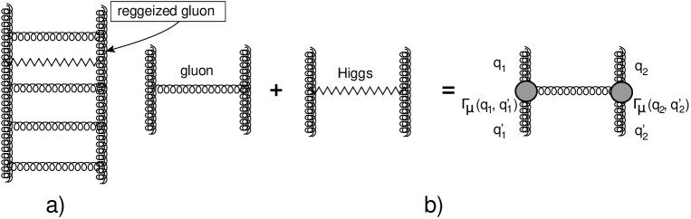
Figure 1: The massive BFKL equation (Fig. 1-a) and its kernel (Fig. 1-b)

The gluon production vertex for the conjugated amplitude can be written as

$$\tilde{\Gamma}_{\mu}\left(q_{2},q_{2}^{\prime}\right)\,\,=\,\,-q^{\perp}_{2,\mu}\,-\,q^{\prime\perp}_{2,\mu}\,+\,p_{1,\mu}\left(-\frac{q^{2}_{2}+m^{2}}{p_{1}\cdot k}\,+\,\frac{p_{2}\cdot k}{p_{1}\cdot p_{2}}\right)\,-\,p_{2,\mu}\left(-\frac{q^{\prime 2}_{2}+m^{2}}{p_{2}\cdot k}\,+\,\frac{p_{1}\cdot k}{p_{1}\cdot p_{2}}\right).$$ (2.2)

Their product is equal to

$$\Gamma_{\mu}\left(q_{1},q_{1}^{\prime}\right)\cdot\tilde{\Gamma}_{\mu}\left(q_{2},q_{2}^{\prime}\right)\,=\,-2\Big{(}\frac{\left(q^{2}_{1}+m^{2}\right)\left(q^{\prime 2}_{2}+m^{2}\right)}{k^{2}+m^{2}}\,\,+\,\,\frac{\left(q^{\prime 2}_{1}+m^{2}\right)\left(q^{2}_{2}+m^{2}\right)}{k^{2}+m^{2}}\Big{)}\,+\,2q^{2}\,+\,3m^{2},$$ (2.3)

where $q_{\mu}\,=\,q_{1,\mu}\,-\,q_{2,\mu}\,=\,q^{\prime}_{1,\mu}\,-\,q^{\prime}_{2,\mu}$.

In the kernel of the BFKL equation ($K^{a^{\prime}b^{\prime}}_{ab}$), corresponding to the real particles in the intermediate state, this product is multiplied by $\alpha_{S}$ and by the corresponding color factor with an additional term from the produced Higgs particles in the singlet and adjoint representations according to the model of Ref.[10] (see Fig. 1-b)

$$K^{a^{\prime}b^{\prime}}_{ab}\,\,\propto\,\,\alpha_{S}\Big{\{}-\frac{1}{2}\Gamma_{\mu}\left(q_{1},q_{1}^{\prime}\right)\cdot\tilde{\Gamma}_{\mu}\left(q_{2},q_{2}^{\prime}\right)f^{ca^{\prime}b^{\prime}}f_{cab}\,\,+\,\,r\,m^{2}\left(\delta_{ab}\,\delta^{a^{\prime}b^{\prime}}\,+\,d^{ca^{\prime}b^{\prime}}d_{cab}\,\frac{N_{c}}{2}\right)\Big{\}}$$ (2.4)

where $f_{cab}$ is the structure constant of the color group $SU(N_{c})$, $d_{abc}$ is the d-coupling tensor and $\delta_{ab}$ is the Kronecker symbol. The coefficient $r$ can be fixed from the bootstrap relation[17]. Due to this relation in the adjoint representation for the $t$ -channel state the real contribution after its partial cancelation with the virtual contribution, corresponding to the Regge trajectories, should be proportional to $q^{2}+m^{2}$. Since the projector on the adjoint representation is $(1/N_{c})f_{caa^{\prime}}f^{cbb^{\prime}}$ we have

$$K^{a^{\prime}b^{\prime}}_{ab}\frac{1}{N_{c}}\,f_{caa^{\prime}}f^{cbb^{\prime}}\,\,\longrightarrow\,\,-\frac{1}{2}\left(2q^{2}+3m^{2}\right)\frac{N_{c}}{2}\,+\,rm^{2}\frac{N^{2}_{c}}{4}\,\,\sim\,\,-\left(q^{2}+m^{2}\right)$$ (2.5)

From Eq. (2.5) we obtain

$$r\,\,=\,\,\frac{1}{N_{c}}$$ (2.6)

and the corresponding contribution to the kernel for the color singlet state in $t$-channel (BFKL Pomeron) is equal to

$$K\left(q_{1},q_{2}|q^{\prime}_{1},q^{\prime}_{2}\right)\,\, = \,\,\frac{\alpha_{S}}{2\pi^{2}}\Big{\{}-\frac{1}{2}N_{c}\Gamma_{\mu}\left(q_{1},q_{1}^{\prime}\right)\cdot\tilde{\Gamma}_{\mu}\left(q_{2},q_{2}^{\prime}\right)\,\,+\,\,\frac{N^{2}_{c}}{4}\,m^{2}\Big{\}}\frac{1}{(q^{\prime 2}_{1}+m^{2})(q^{\prime 2}_{2}+m^{2})}$$

$$= \frac{\alpha_{S}N_{c}}{2\pi^{2}}\Big{\{}\frac{1}{k^{2}+m^{2}}\Big{(}\frac{q^{2}_{1}+m^{2}}{q^{\prime 2}_{1}+m^{2}}\,+\,\frac{q^{2}_{2}+m^{2}}{q^{\prime 2}_{2}+m^{2}}\Big{)}\,\,-\,\,\frac{q^{2}+\frac{N^{2}_{c}+1}{N^{2}_{c}}m^{2}}{(q^{\prime 2}_{1}+m^{2})(q^{\prime 2}_{2}+m^{2})}\Big{\}}$$

In the integral form the homogeneous BFKL equation at $q=0$ for the Yang-Mills theory with the Higgs mechanism is given by

$$\omega f\left(p\right)\,\,=\,\,2\omega\left(p\right)f\left(p\right)\,+\,\frac{\alpha_{S}N_{c}}{2\pi^{2}}\int d^{2}p^{\prime}\Big{(}\frac{2f\left(p^{\prime}\right)}{\left(\vec{p}-\vec{p}^{\,\,{}^{\prime}}\right)^{2}+m^{2}}\,\,-\,\,\frac{\frac{N^{2}_{c}+1}{N^{2}_{c}}m^{2}\,f\left(p^{\prime}\right)}{(p^{2}+m^{2})(p^{\prime 2}+m^{2}}\Big{)}$$ (2.8)

where we use the following notations: $q_{1}=q_{2}=p$ and $q^{\prime}_{1}=q^{\prime}_{2}=p^{\prime}$.

The gluon Regge trajectory ($\omega\left(p\right)$) is calculated explicitly,

$$\omega\left(|p|\right)\,\, = \,\,-\frac{\alpha_{S}N_{c}}{4\pi^{2}}\int\frac{d^{2}k\left(p^{2}+m^{2}\right)}{\left(k^{2}+m^{2}\right)\left(\left(\vec{p}-\vec{k}\right)^{2}+m^{2}\right)}$$ (2.9)

$$= \,\,-\frac{\alpha_{S}N_{c}}{2\pi^{2}}\frac{|p|^{2}+m^{2}}{|p|\sqrt{|p|^{2}+4m^{2}}}\ln\frac{\sqrt{|p|^{2}+4m^{2}}+|p|}{\sqrt{|p|^{2}+4m^{2}}-|p|}$$

Assuming that we search the rotationally symmetric solution, the kernel can be averaged over the azimuthal angle $\phi$

$$\int^{2\pi}_{0}\frac{d\phi}{2\pi}\,\frac{1}{p^{2}+p^{\prime 2}+m^{2}-2|p||p^{\prime}|\cos\phi}\, = \,\frac{1}{\sqrt{\left(p^{2}+p^{\prime 2}+m^{2}\right)^{2}-4p^{2}p^{\prime 2}}}$$ (2.10)

$$= \,\frac{1}{\sqrt{\left(p^{2}-p^{\prime 2}\right)^{2}\,+\,2\left(p^{2}+p^{\prime 2}\right)m^{2}\,+\,m^{4}}}$$

Introducing the new variables

$$\kappa\,=\,\frac{p^{2}}{m^{2}};\,\,\,\,\,\,\,\,\,\,\,\,\,\,\kappa^{\prime}\,=\,\frac{p^{\prime 2}}{m^{2}};\,\,\,\,\,\,\,\,\,\,\,\,\,E\,=\,-\frac{\omega}{\bar{\alpha}_{S}};\,\,\,\,\,\,\,\,\,\,\,\,\,\bar{\alpha}_{S}\,=\,\frac{\alpha_{S}N_{c}}{\pi}$$ (2.11)

we obtain the one-dimensional BFKL equation

$$E\phi\left(\kappa\right)\,\,=$$ (2.12)

$$\,\,\underbrace{\frac{\kappa+1}{\sqrt{\kappa}\sqrt{\kappa+4}}\ln\frac{\sqrt{\kappa+4}+\sqrt{\kappa}}{\sqrt{\kappa+4}-\sqrt{\kappa}}\phi\left(\kappa\right)}_{{\rm kinetic\,energy\,term}}\,\,-\,\,\underbrace{\int^{\infty}_{0}\,\frac{d\kappa^{\prime}\phi\left(\kappa^{\prime}\right)}{\sqrt{(\kappa-\kappa^{\prime})^{2}\,+\,2(\kappa+\kappa^{\prime})+1}}}_{\rm potential\,energy\,term}\,\,+\,\,\underbrace{\frac{N^{2}_{c}+1}{2N^{2}_{c}}\frac{1}{\kappa+1}\int^{\infty}_{0}\frac{\phi\left(\kappa^{\prime}\right)\,d\kappa^{\prime}}{\kappa^{\prime}+1}}_{{\rm contact\,term}}$$

3 Solution to the massive BFKL equation

3.1 General features of the equation

We start to discuss the solution to the equation considering the most general properties of solutions. At large $\kappa$ solutions to this equation should coincide with the solution to the BFKL equation with $m=0$ which has the following form:

$$E\,\phi_{\mbox{\tiny BFKL}}\left(\kappa\right)\,\,=\,\,\ln\kappa\,\phi_{\mbox{\tiny BFKL}}\,\,-\,\,\int^{\infty}_{0}\,\frac{d\kappa^{\prime}\,\phi_{\mbox{\tiny BFKL}}\left(\kappa^{\prime}\right)}{|\kappa-\kappa^{\prime}|}$$ (3.13)

after an appropriate regularization of divergency at $\kappa^{\prime}=\kappa$ (see [10]).”

The eigenvalues and the eigenfunctions of this equation are well known [10, 11]. Therefore, the solution to Eq. (2.12) has the following large $\kappa$ behaviour

$$\phi\left(\kappa\right)\,\,\xrightarrow{\kappa\to\infty}\,\,\phi_{\mbox{\tiny BFKL}}\left(\kappa\right)\,\sim\,\kappa^{-\frac{1}{2}+i\nu}\,\,\,\,\,\,\mbox{with}\,\,\,\,\,\,E\left(\nu\right)\,\,=\,\,\chi\left(\nu\right)\,\,=\,\,\psi\left(\frac{1}{2}+i\nu\right)\,+\,\psi\left(\frac{1}{2}-i\nu\right)\,-\,2\psi\left(1\right)$$ (3.14)

where $\psi(z)=d\ln\Gamma(z)/dz$ ( see formulae 8.36 in Ref.[19]).

Looking at Eq. (2.12) one can conclude that $\phi\left(\kappa\right)$ should be analytical functions with a cut at $\kappa<-4$ and pole at $\kappa=-1$.

We find instructive to re-write Eq. (2.8) in the coordinate representation.

Using an identity

$$\int\frac{d^{2}p^{\prime}}{2\pi}\frac{e^{i\vec{r}\cdot\vec{p}^{\,\,{}^{\prime}}}}{p^{\prime 2}+m^{2}}\,=\,\int^{+\infty}_{-\infty}\frac{p^{\prime}dp^{\prime}\,J_{0}\left(rp^{\prime}\right)}{p^{\prime 2}+m^{2}}\,\,=\,\,K_{0}\left(rm\right)$$ (3.15)

where $J_{0}\left(z\right)$ and $K_{0}\left(z\right)$ are the Bessel and Macdonald functions [19], we can rewrite Eq. (2.8) in the form

$$E\,f\left(r\right)\,\,=\,\,{\cal H}\,f\left(r\right)$$ (3.16)

with

$${\cal H}\,=\,\frac{p^{2}+m^{2}}{|p|\sqrt{p^{2}+4m^{2}}}\ln\frac{\sqrt{p^{2}+4m^{2}}+|p|}{\sqrt{p^{2}+4m^{2}}-|p|}\,\,-\,\,2K_{0}\left(|r|m\right)\,+\,\frac{N^{2}_{c}+1}{2\,N^{2}_{c}}\hat{P}\,\,=\,\,T\left(p\right)\,\,+\,\,V\left(r\right)\,\,+\,\,\frac{N^{2}_{c}+1}{2\,N^{2}_{c}}\hat{P}$$ (3.17)

where $\hat{P}$ is a shorthand notation for the projector onto the state $\sim m^{2}/(p^{2}+m^{2})$

$$\hat{P}\,\phi\left(p\right)\,=\,\frac{m^{2}}{p^{2}+m^{2}}\int\frac{d^{2}p^{\prime}}{\pi}\frac{\phi\left(p^{\prime}\right)}{p^{\prime 2}\,+\,m^{2}}$$ (3.18)

Let us introduce as a free Hamiltonian, the Hamiltonian for the massless BFKL equation (see Eq. (3.13):

$${\cal H}_{0}\,=\,\ln p^{2}\,+\,\ln|r|^{2}\,-\,2\psi\left(1\right)\,=\,\frac{1}{2}\left(\psi\left(1+x\partial\right)\,+\,\psi\left(-x\partial\right)\,+\,\psi\left(1+x^{*}\partial^{*}\right)\,+\,\psi\left(-x^{*}\partial^{*}\right)\,-\,4\psi\left(1\right)\right)$$ (3.19)

Since this Hamiltonian operates in the two-dimensional transverse plane, it is convenient to deal with the components of all vectors as real and imaginary parts of the complex numbers, namely

$$x\,=\,r_{1}+ir_{2};~{}~{}~{}~{}~{}~{}x^{*}\,=\,r_{1}-ir_{2};;~{}~{}~{}~{}~{}~{}\vec{p}\,=\,-i\vec{\nabla}\,=\,\left(-i\partial-i\partial^{*},\,\partial-\partial^{*}\right)$$ (3.20)

where the indices 1 and 2 denote the two transverse axes.

The eigenfunctions with the conformal spin $n=0$ take the form (see Ref.[11])

$$f^{\pm\nu}_{0}\left(|r|\right)\,\,=\,\,|r|^{-1\pm 2i\nu}$$ (3.21)

with the eigenvalues $E\left(\nu\right)$ given by Eq. (3.14). The eigenfunctions of Eq. (3.21) have the following orthogonality and completeness properties

$$\int^{\infty}_{0}d|r|^{2}f^{\nu}_{0}\left(|r|\right)f^{\mu*}_{0}\left(|r|\right)\,\, = \,\,2\pi\delta\left(\mu-\nu\right)\,;$$ (3.22)

$$|r||r^{\prime}|\int^{+\infty}_{-\infty}d\nu f^{\nu}_{0}\left(|r|\right)f^{\nu*}_{0}\left(|r^{\prime}|\right)\,\, = \,\,2\pi\delta\left(\ln|r|^{2}\,-\,\ln|r^{\prime}|^{2}\right)\,.$$ (3.23)

The Green function for the free Hamiltonian satisfies the following equation

$$\left(E\,-\,{\cal H}_{0}\right)G_{0}\left(r,r^{\prime}\right)\,\,=\,\,\frac{2\pi}{|r||r^{\prime}|}\delta\left(\ln|r|^{2}\,-\,\ln|r^{\prime}|^{2}\right)$$ (3.24)

and it has the form

$$G_{0}\left(r,r^{\prime}\right)\,\,=\,\,\frac{1}{|r||r^{\prime}|}\int^{+\infty}_{-\infty}\frac{d\nu}{E\,-\,E\left(\nu\right)}\left(\frac{|r|}{|r^{\prime}|}\right)^{2i\nu}$$ (3.25)

The Green function for the general Hamiltonian of Eq. (3.16) can be found as a solution to the integral equation

$$G\left(r,r^{\prime}\right)\,\,=\,\,G_{0}\left(r,r^{\prime}\right)\,\,+\,\,\int dr^{\prime\prime}G_{0}\left(r,r^{\prime\prime}\right)\,\,\Big{(}{\cal H}\,-\,{\cal H}_{0}\Big{)}G\left(r^{\prime\prime},r^{\prime}\right)$$ (3.26)

Eq. (3.26) gives a natural way for applying a perturbative approach. In particular, in the lowest order of expansion with respect to $m^{2}$ we have

$${\cal H}\,-\,{\cal H}_{0}\,\,=\,\,\frac{m^{2}}{p^{2}}\Big{(}-\ln\frac{p^{2}}{m^{2}}+2\Big{)}\,+\,\frac{m^{2}r^{2}}{4}\Big{(}\ln\frac{r^{2}}{4}-2\psi\left(2\right)\Big{)}\,+\,\frac{N^{2}_{c}+1}{2\,N^{2}_{c}}\hat{P}\,\,+\,\,{\cal O}\left(m^{4}\right)$$ (3.27)

At large distances ($r\to\infty$) the potential energy in Hamiltonian $\left(V\left(r\right)=-2K_{0}\left(rm\right)\right)$ is exponentially small, the contribution from the projector $\hat{P}$ in Eq. (3.16) is proportional to $1/(p^{2}+m^{2})$ and is also exponentially suppressed, so the only relevant term in the hamiltonian is the kinetic energy

$$E\left(p\right)\,\,=\,\,T\left(p\right)\,\,=\,\,\frac{p^{2}+m^{2}}{|p|\sqrt{p^{2}+4m^{2}}}\ln\frac{\sqrt{p^{2}+4m^{2}}+|p|}{\sqrt{p^{2}+4m^{2}}-|p|},$$ (3.28)

for which the eigenfunctions have a form

$$f\left(\vec{r}\right)\,\,\sim\,\,e^{i\sqrt{p^{2}}r},p^{2}>0,\quad f\left(\vec{r}\right)\,\,\sim\,\,e^{-\sqrt{-p^{2}}r},p^{2}<0.$$ (3.29)

The point $p=0$ is special since it separates two different behaviours at large $r$. This point corresponds to energy $E=\frac{1}{2}$ or $\omega=\omega_{0}\equiv-\frac{1}{2}\bar{\alpha}_{S}$. As we will see below, there are qualitative changes in the shape of the wave functions near this point. From the structure of the kinetic energy term (3.28) we can see that the energy $E$ is positive ($\omega<0$) for $p^{2}>0$, however for $-4m^{2}<p^{2}<0$ the energy may have any value from $-\infty$ up to $\frac{1}{2}$. In reality the spectrum $E$ is limited from below by $-4\ln 2$, as it is shown in sections 3.2 and 3.3.

In the small-$r$ limit the eigenfunctions should approach the eigenfunctions of the massless BFKL equations, $f^{\pm\nu}_{0}\left(|r|\right)$ Eq. (3.21), with the spectrum given by Eq. (3.14).

Combining Eq. (3.21) and Eq. (3.28), we may get the relation between the parameters $\nu$ and $p$, which control the the small-$r$ and large-$r$ asymptotic behaviour,

Figure 2: The dependence of the kinetic energy (see Eq. (3.28)) versus $p^{2}$ for $m=1$.

$$E=T(p)=\chi(\nu)$$ (3.30)

3.2 Estimates from the variational method

In the variational approach the upper bound for the ground state energy $E_{0}$ of the hamiltonian $\mathcal{H}$ may be found minimizing the functional

$$E_{\mbox{ground}}\,\,\equiv\,\,E_{0}\,\,\,\leq\,\,\,F[\{\phi\}]\,\,=\,\,\frac{\Big{\langle}\phi^{\ast}\!\left(r\right)\Big{|}{\cal H}\Big{|}\phi\!\left(r\right)\Big{\rangle}}{\Big{\langle}\phi^{\ast}\!\left(r\right)\Big{|}\phi\!\left(r\right)\Big{\rangle}}$$ (3.31)

Eq. (3.31) means that the functional $F[\{\phi\}]$ has a minimum for function $\phi_{0}\left(r\right)$ which is the eigenfunction of the ground state with energy $E_{0}$.

For our Hamiltonian in the momentum space Eq. (3.31) can be re-written in the form

$$E_{0}\,\,=\,\,\min_{\phi}\frac{\int^{\infty}_{0}d\kappa\,T\left(\kappa\right)\,|\phi\left(\kappa\right)|^{2}\,-\,\int^{\infty}_{0}d\kappa\int^{\infty}_{0}d\kappa^{\prime}\frac{\phi\left(\kappa\right)\phi^{*}\left(\kappa^{\prime}\right)}{\sqrt{\left(\kappa-\kappa^{\prime}\right)^{2}+2\left(\kappa+\kappa^{\prime}\right)+1}}\,+\,\frac{N^{2}_{c}+1}{2N^{2}_{c}}\Big{|}\int^{\infty}_{0}d\kappa\,\frac{\phi\left(\kappa\right)}{\kappa+1}\Big{|}^{2}}{\int^{\infty}_{0}d\kappa|\phi\left(\kappa\right)|^{2}}$$ (3.32)

The success of finding the value of $E_{0}$ depends on the choice of the trial functions in Eq. (3.32). We choose it in the form

$$\phi_{\mbox{trial}}\left(\kappa\right)\,\,=\,\,\frac{1}{\left(\kappa+a^{2}\right)^{\gamma}}$$ (3.33)

In the coordinate representation Eq. (3.33) corresponds to

$$f_{\mbox{trial}}\left(r\right)\,\,=\,\,\frac{1}{\Gamma\left(\gamma\right)}\left(\frac{r}{2a}\right)^{-1+\gamma}\,K_{1-\gamma}\left(ar\right)\,\,\rightarrow\,\,\left\{\begin{array}[]{l l}r\,\rightarrow\infty&\,\,\,\propto~{}~{}r^{-\gamma}e^{-a|r|}\\ &\\ r\,\rightarrow\,\,0&\,\,\,\propto\,~{}~{}r^{-2+2\gamma}\end{array}\right.$$ (3.34)

One can see that our trial function has the correct behaviour if $a>0$ and $b\,=\,2\gamma-1\,>\,0$.

Fig. 3-a		Fig. 3-b

Figure 3: Dependence of $E_{0}$ given by Eq. (3.32) on $\gamma$ (see Fig. 3-a) and $a$(see Fig. 3-b). The red straight line corresponds to the ground state energy of the massless BFKL equation $E_{\mbox{\tiny BFKL}}\,\,=\,\,-4\ln 2$.

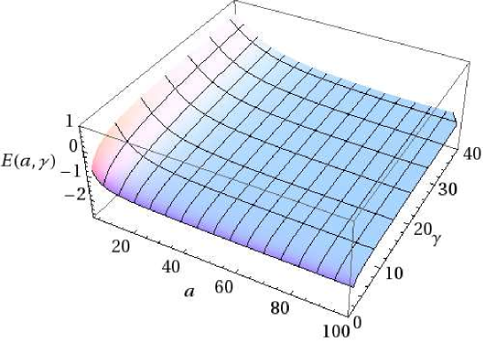
Figure 4: The dependence of the energy given by Eq. (3.32) on the values of parameters $a$ and $\gamma$.

Fig. 3 shows the dependence of $E_{0}$ on $\gamma$ and $a$. At large $a$ and $\gamma\to 0.5$, $E_{0}$ reaches minimum value which is the massless BFKL energy $E_{BFKL}$. Therefore, we conclude that the ground state energy $E_{0}$ could be only smaller than $E_{BFKL}$ but not larger than it. Fig. 4 demonstrates the global tendency in the dependence of $E_{0}$ on the values of parameters $a$ and $\gamma$. Similar results were obtained for more complicated parameterizations like

$$\phi(\kappa)=\frac{\kappa^{-\delta}}{\left(\kappa+a^{2}\right)^{\gamma}},$$ (3.35)

$$\phi(\kappa)=\frac{\kappa^{-\delta}}{\left(\kappa+a^{2}\right)^{3/2}\left(\kappa+b^{2}\right)^{\gamma-3/2}}.$$ (3.36)

While from the variational principle we always obtained the energy $E>E_{BFKL}$, we believe that the true minimum of the energy is $E=E_{BFKL}$ (respectively the eigenvalue $\omega=\omega_{BFKL}$), there is no indication that there are eigenvalues with $\omega>\omega_{BFKL}$. Actually, with trial function of Eq. (3.33) for $a\gg 1$ we can perform the analytical calculation(see appendix) which shows that at $\gamma=1/2$ we indeed have the minimum with $\omega=\omega_{\mbox{\tiny BFKL}}$.

3.3 Independence of the Pomeron spectrum from the gluon mass

In this section we wish to prove that there are no Pomeron states above the intercept of the massless BFKL equation. As we have seen in the variational approach, the best trial function that describes the BFKL Pomeron takes the form

$$\phi^{0}_{\mbox{\tiny trial}}\,\,=\,\,\frac{1}{\sqrt{\kappa\,\,+\,\,a^{2}}}$$ (3.37)

It gives $E_{\mbox{\tiny BFKL}}\,\,=\,\,-\,4\,\ln 2$ independently from $a$ (see Fig. 3-a). We wish to prove that

$$E\,\,\geq\,\,E_{\mbox{\tiny BFKL}}\,\,=\,\,-\,4\,\ln 2$$ (3.38)

Since the energy contribution of the contact term is positive, we neglect it below.

For the proof of (3.38) we re-write the Hamiltonian of Eq. (3.17) in the form

$${\cal H}\,\,=\,\,T\left(p\right)\,\,+\,\,V\left(r\right)\,\,=\,\,\Big{\{}T\left(p\right)\,\,-\,\,T_{0}\left(p\right)\Big{\}}\,\,+\,\,{\cal H}_{0}$$ (3.39)

where ${\cal H}_{0}$ is chosen from the condition

$${\cal H}_{0}\phi^{0}_{\mbox{\tiny trial}}\,\,=\,\,\Big{(}T_{0}\left(p\right)\,\,+\,\,V\left(r\right)\Big{)}\phi^{0}_{\mbox{\tiny trial}}\,\,=\,\,E_{\mbox{\tiny BFKL}}\phi^{0}_{\mbox{\tiny trial}}$$ (3.40)

If we verify that $\{T(p)-T_{0}(p)\}\geq 0$ for all values of $p$, then inequality (3.38) is valid due to (3.40) because $\phi^{0}_{trial}$ is positive for the ground state of $H_{0}$.

Neglecting the contact term, the kinetic energy $T_{0}(p)$ takes the form

$$T_{0}\left(p\right)\,\,=\,\,E_{\mbox{\tiny BFKL}}\,\,-\,\,\frac{1}{\phi^{0}_{\mbox{\tiny trial}}\left(p\right)}V(r)\phi^{0}_{\mbox{\tiny trial}}\left(r\right)\,$$ (3.41)

where

$$\frac{1}{\phi^{0}_{\mbox{\tiny trial}}\left(p\right)}V(r)\phi^{0}_{\mbox{\tiny trial}}\left(r\right)\,=\,-\int\frac{d^{2}p^{\prime}}{\pi}\frac{\sqrt{p^{2}+a^{2}}}{(|\vec{p}-\vec{p}^{\,{}^{\prime}}|^{2}+1)\sqrt{p^{\prime 2}+a^{2}}}=-\int_{0}^{1}\frac{d\beta}{\sqrt{1-\beta}}\,\frac{\sqrt{p^{2}+a^{2}}}{\sqrt{\beta(1-\beta)p^{2}+a^{2}(1-\beta)+\beta}}\,$$ (3.42)

The last expression can be written in terms of the elliptic integral in the Weierstrass form or in the Jacobi form after the following transformation

$$\frac{1}{\phi^{0}_{\mbox{\tiny trial}}\left(p\right)}V(r)\phi^{0}_{\mbox{\tiny trial}}\left(r\right)\,\,=\,\,-2\int_{0}^{1}dz\frac{\sqrt{p^{2}+a^{2}}}{\sqrt{z^{2}(1-z^{2})p^{2}+a^{2}\,z^{2}+1-z^{2}}}\,.$$ (3.43)

For Eq. (3.43) we can find the asymptotic behaviour for large and small $p$, viz.

$$\frac{1}{\phi^{0}_{\mbox{\tiny trial}}\left(p\right)}V(r)\phi^{0}_{\mbox{\tiny trial}}\left(r\right)\,\,~{} \xrightarrow{p\,\,\gg\,\,1} ~{}~{}-\frac{2}{p}\,\ln p-4\ln 2+\frac{\ln p}{p^{2}}\,\left(-\frac{1}{2}+a\right)+{\cal O}(1/p^{2});$$ (3.44)

$$\xrightarrow{p\,\,\to\,\,0} ~{}~{}-\,\frac{2\sqrt{a^{2}}}{\sqrt{a^{2}\,-\,1}}\,\ln(\sqrt{a^{2}\,-\,1}+\sqrt{a^{2}})$$ (3.45)

In terms of $\Big{\{}T\left(p\right)\,\,-\,\,T_{0}\left(p\right)\Big{\}}$ it means that

$$\Big{\{}T\left(p\right)\,\,-\,\,T_{0}\left(p\right)\Big{\}}~{}~{} \xrightarrow{p\,\gg\,1} ~{}~{}\frac{\ln p}{p}\,\left(a-\frac{5}{2}\right);$$ (3.46)

$$\xrightarrow{p\,\to\,0} ~{}~{}\frac{1}{2}+4\ln 2\,-\,2\sqrt{\frac{a^{2}}{a^{2}-1}}\,\ln(\sqrt{a^{2}-1}+\sqrt{a^{2}}).$$ (3.47)

As a result, it is plausible, that $T(p)-T_{0}(p)$ is positive for all $p$ providing that the parameter $a$ lies in the interval

$$\frac{5}{2}\,<\,a^{2}\,<\,a^{2}_{0}\,,$$ (3.48)

where $a_{0}$ is found from the equation

$$\frac{1}{2}\,+\,4\ln 2\,\,-2\sqrt{\frac{a^{2}_{0}}{a^{2}_{0}-1}}\,\ln(\sqrt{a^{2}_{0}-1}+\sqrt{a^{2}_{0}})=0\,.$$ (3.49)

which gives $a^{2}_{0}=5.26$.

In Fig. 5 we calculated the difference $T\left(p\right)\,\,-\,\,T_{0}\left(p\right)$ using the integral of Eq. (3.42) and/or Eq. (3.43) without expansion of Eq. (3.46) and Eq. (3.47). One can see that for $5\,>\,a^{2}\,>\,0$ at any values of $p$ this difference is positive.

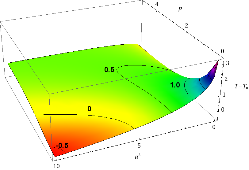
Figure 5: The dependence of $T\left(p\right)\,\,-\,\,T_{0}\left(p\right)$ on the values of parameter $a$ and $p$.

The condition of the minimum of $|T(p)-T_{0}(p)|$ should be used in the variational approach for fixing the unique wave function, because the minimum of energy is realized on many configurations.

Fig. 6 shows that the condition of Eq. (3.30): $E=T\left(p\right)=T\left(ia\right)$, is fulfilled for $a$ in the interval of Eq. (3.48)(or Fig. 5). Thus, inequality (3.38) is proven.

Figure 6: The dependence of $T\left(ia\right)$ on the values of parameter $a$ (solid line) and $E=-\chi(0)=-4\ln 2$ (dotted line).

3.4 Relation between energy and wave function

In this section we demonstrate that the value of energy $E\left(\beta\right)$ is completely determined by the asymptotic behavior of the wave function at large $p$ for a more general trial function of the form

$$\phi_{\mbox{trial}}\left(p\right)\,\,=\,\,\left(p^{2}\,\,+\,\,a^{2}\right)^{-\frac{1}{2}\,+\,i\beta}.$$ (3.50)

This proof complements the proof given in section 3.1, in which we used properties of the massless BFKL equation and argued that the spectrum of massless and massive BFKL kernels should coincide at large $p$. The trial function Eq. (3.50) is close to the wave functions which we will obtain numerically in section 3.6, so we find it instructive to repeat the proof for these functions in a more transparent way.

For the trial function of Eq. (3.50) Eq. (3.48) takes the form

$$\frac{V(r)\phi_{\mbox{\tiny trial}}\left(r\right)}{\phi_{\mbox{\tiny trial}}\left(p\right)}\, =$$

$$- \int\frac{d^{2}p^{\prime}}{\pi}\frac{\left(p^{2}+a^{2}\right)^{\frac{1}{2}+i\beta}}{(|\vec{p}-\vec{p}^{\,{}^{\prime}}|^{2}+1)\left(p^{\prime 2}+a^{2}\right)^{\frac{1}{2}+i\beta}}=-\int_{0}^{1}\frac{dx}{\sqrt{1-\beta}}\,\frac{\left(p^{2}+a^{2}\right)^{\frac{1}{2}+i\beta}}{\left(\beta(1-x)p^{2}+a^{2}(1-x)+x\right)^{\frac{1}{2}+i\beta}}$$

We introduced Feynman parameter $x$ and integrated over $p^{\prime}$ to obtain the last equation in Eq. (3.4).

For large $p$ the essential region of integration is $a^{2}/p^{2}\leq x\leq 1$. We introduce an intermediate parameter $\sigma$ with its value in the interval $a^{2}/p^{2}\,\ll\,\sigma\,\ll\,1$ and rewrite Eq. (3.4) in the form

$$\frac{V(r)\phi_{\mbox{\tiny trial}}\left(r\right)}{\phi_{\mbox{\tiny trial}}\left(p\right)}\,=$$ (3.52)

$$-\int^{\sigma}_{0}\frac{dx}{x}\frac{1}{\left(1+\frac{1}{xp^{2}}\right)^{\frac{1}{2}+i\beta}}\,\,-\,\,\int^{1}_{\sigma}\frac{dx}{x}\frac{1}{\left(1-x\right)^{\frac{1}{2}+i\beta}}\,\,=\,\,-\int^{\infty}_{1+\frac{1}{\sigma p^{2}}}\frac{dz}{\left(z-1\right)}\,\,\frac{1}{z^{\frac{1}{2}+i\beta}}\,\,-\,\,\int^{1}_{\sigma}\frac{dx}{x}\frac{1}{\left(1-x\right)^{\frac{1}{2}+i\beta}}$$

$$=\,\,-\int^{1-\frac{1}{\sigma p^{2}}}_{0}\frac{dt}{t(1-t)}\,t^{\frac{1}{2}+i\beta}\,\,-\,\,\int^{1-\sigma}_{0}\frac{dt}{1-t}\,t^{-\frac{1}{2}-i\beta}\,\,=\,\,-\ln p^{2}\,\,-\,\,\int^{1}_{0}\,dt\frac{t^{-\frac{1}{2}}\left(t^{-i\beta}+t^{i\beta}\right)-2}{(1-t)}$$

Therefore,

$$E\left(\beta\right)\,\,=\,\,\psi\left(\frac{1}{2}+i\beta\right)\,\,+\,\,\psi\left(\frac{1}{2}-i\beta\right)\,\,-\,\,2\,\psi\left(1\right)$$ (3.53)

independently of the value of $a$. Moreover, the result for the energy $E\left(\beta\right)$ does not depend on the form of wave function providing that it has the correct asymptotic behavior at large $p$ . For example, the wave function $\phi^{(approx)}_{n}\left(\kappa\right)$ of Eq. (3.62) that stems from our numerical estimates, can be written as the real part of the expression

$$\phi^{(approx)}_{n}\left(\kappa\right)\,\,=\,\,\frac{e^{i\varphi}}{\sqrt{\kappa+4}}\left(\frac{\sqrt{\kappa+4}+\sqrt{\kappa}}{\sqrt{\kappa+4}-\sqrt{\kappa}}\right)^{-i\beta}$$ (3.54)

The difference of energy for the wave functions of Eq. (3.50) and Eq. (3.54) takes the form

$$\Delta E\left(\beta\right)\,\,=\,\,\int\frac{d^{2}p^{\prime}}{\pi}\frac{p^{2(\frac{1}{2}+i\beta)}}{\left(|\vec{p}-\vec{p}^{\,{}^{\prime}}|^{2}+1\right)\sqrt{p^{\prime 2}+4}}\left(\frac{1}{\left(p^{\prime 2}+4\right)^{i\beta}}\,\,-\,\,\left(\frac{\sqrt{p^{\prime 2}+4}+\sqrt{p^{\prime 2}}}{\sqrt{p^{\prime 2}+4}-\sqrt{p^{\prime 2}}}\right)^{-i\beta}\right)$$ (3.55)

From the dimensional considerations $\Delta E\left(\beta\right)$ falls down as $1/p^{2}$ at large $p$ and therefore, the energies $E\left(\beta\right)$ for wave function of Eq. (3.50) and Eq. (3.54) coincide.

3.5 Numerical solution

3.5.1 Direct method

3.5.1.1 General approach.

Eq. (2.12) and Eq. (3.13) have the following structure

$$\omega\,\phi\left(\kappa\right)\,\,=\,\,\bar{\alpha}_{S}\,\int d\kappa^{\prime}K\left(\kappa,\kappa^{\prime}\right)\,\phi\left(\kappa^{\prime}\right)$$ (3.56)

Notice that we re-write Eq. (2.12) and Eq. (3.13) in terms of $\omega$ and restore the coupling constant in front of the integral. In the numerical calculation we replace the continuous variables $\kappa$ and $\kappa^{\prime}$ by the discrete set of $\{\kappa_{n}\}$ and $\{\kappa^{\prime}_{n}\}$ using the logarithmic grid (in $\kappa=k^{2}/m^{2}$) with $N+1$ nodes,

$$\kappa_{n} = \kappa_{min}\exp\left(\frac{n}{N}\,\ln\left(\kappa_{max}/\kappa_{min}\right)\right),\quad n=0,...,N,$$ (3.57)

where the values of $\kappa_{min},\,\kappa_{max}$ were set to $\kappa_{min}=10^{-40},\kappa_{max}=10^{80}$, and $N=1024$.

In the discrete variables Eq. (3.56) takes the form

$$\omega\phi\left(\kappa_{n}\right)\,\,=\,\,\bar{\alpha}_{S}\sum^{N}_{m=0}K\left(\kappa_{n},\kappa^{\prime}_{m}\right)\,\kappa^{\prime}_{m}\,\left(\frac{1}{N}\,\ln\left(\kappa_{max}/\kappa_{min}\right)\right)\,\phi\left(\,\kappa^{\prime}_{m}\right)$$ (3.58)

where $\kappa_{n}$ and $\kappa^{\prime}_{m}$ are taken in the form of Eq. (3.57). Introducing the notations: $\phi\left(\kappa_{n}\right)\equiv\phi_{n}$ and $K\left(\kappa_{n},\kappa^{\prime}_{m}\right)\kappa^{\prime}_{m}\,\left(\frac{1}{N}\,\ln\left(\kappa_{max}/\kappa_{min}\right)\right)\,\equiv\,{\cal K}_{nm}$ we can re-write Eq. (3.58) in the matrix form

$$\omega\,\phi_{n}\,\,=\,\,\bar{\alpha}_{S}\sum^{N}_{m=0}{\cal K}_{nm}\,\phi_{m}~{}~{}~{}~{}~{}~{}~{}~{}\mbox{or}~{}~{}~{}~{}~{}~{}~{}~{}~{}\omega\,\vec{\phi}\,\,=\,\,\bar{\alpha}_{S}\,{\cal\mathbf{K}}\,\vec{\phi}$$ (3.59)

where vector $\vec{\phi}$ has $N+1$ components $\phi_{n}$ and ${\cal\mathbf{K}}$ is $(N+1)\times(N+1)$ matrix. To find the roots of the characteristic polynomial $p\left(\omega\right)$ of the matrix $\bar{\alpha}_{S}\,{\cal\mathbf{K}}\,-\,\omega{\mathbf{I}}$, where ${\mathbf{I}}$ is the identity matrix, we need to solve the secular equation

$$p\left(\omega\right)\,\,=\,\,\mbox{det}\left(\bar{\alpha}_{S}\,{\cal\mathbf{K}}\,-\,\omega{\mathbf{I}}\right)\,\,=\,\,0$$ (3.60)

We use Eq. (3.59) and Eq. (3.60) to find the eigenvalues and eigenfunctions both for massive (2.12) and massless (3.13) BFKL equations, using the analytic solution Eq. (3.14) to control the accuracy of our numerical calculations. Due to finite grid size, the spectrum is discrete, with a few positive roots given in the Table 1 and Fig. 7. Sensitivity to a number of points is quite mild, so discretization error should be small. As one can see from the Fig. 7, when $\kappa_{max}$ grows up to infinity, the distance between the roots decreases rapidly, with the highest root asymptotically approaching the massless BFKL value $\omega_{\mbox{\tiny BFKL}}\,=\,4\,\bar{\alpha}_{S}\,\ln 2\,\,\,\approx\,\,0.56$ for $\bar{\alpha}_{S}=0.2$, both for the massive and massless cases. It should be stressed that the relative difference between the highest eigenvalue in our calculation for the massless BFKL equation and the exact $\omega_{BFKL}$ is negligibly small (of the order of $3\times 10^{-5}$), which demonstrates a good accuracy of a chosen method. We found that the eigenvalues of the massless BFKL equation can be written in a familiar form

$$\omega_{n}\left(m=0\right)\,\, = \,\,\bar{\alpha}_{S}\left(2\psi\left(1\right)\,-\,\psi\left(\frac{1}{2}-i\beta_{n}(m=0)\right)\,-\,\psi\left(\frac{1}{2}+i\beta_{n}(m=0)\right)\right)$$ (3.61)

with $$~{}~{}~{}~{}~{}\beta_{n}(m)\,=\,a\left(m\right)\,n,~{}~{}~{}~{}~{}\qquad~{}~{}~{}~{}\,a\left(m\right)\,=\,2.9/\ln\left(\kappa_{\mbox{max}}/\left(\kappa_{\mbox{min}}\,+\,m^{2}\right)\right),$$

and $\kappa_{\mbox{max}}$ and $\kappa_{\mbox{min}}$ are the upper and lower cutoffs introduced in Eq. (3.57).

Root #	$\omega_{n}^{(BFKL)}$	$\omega_{n}^{(mass)}$		Root #	$\omega_{n}^{(BFKL)}$	$\omega_{n}^{(mass)}$
1	0.5545	0.554		11	0.507	0.454
2	0.553	0.551		12	0.499	0.437
3	0.551	0.547		13	0.489	0.420
4	0.548	0.540		14	0.480	0.402
5	0.545	0.532		15	0.470	0.383
6	0.540	0.522		16	0.459	0.365
7	0.535	0.511		17	0.448	0.346
8	0.529	0.498		18	0.437	0.327
9	0.522	0.485		19	0.426	0.308
10	0.515	0.470		20	0.414	0.289

Table 1: The first twenty roots of the original (massless) BFKL equation (column $\omega_{n}^{(BFKL)}$) and BFKL with mass (column $\omega_{n}^{(mass)}$) found with the chosen method. Note that for the first root for the massless BFKL, we get $\omega_{0}^{BFKL}\,\approx\,0.554504$, whereas the true value is $4\bar{\alpha}\ln 2\,\approx\,0.554518$, i.e. the relative difference is of order $3\times 10^{-5}$.

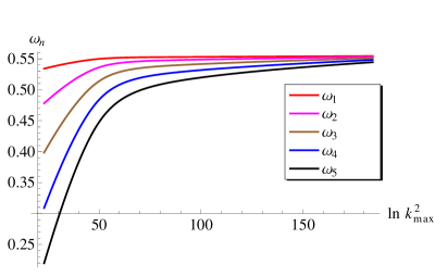
Figure 7: Dependence of the first 5 eigenvalues on the maximal cutoff $\kappa_{max}=k_{max}^{2}$.

In Fig. 8 one can see how the simple formula of Eq. (3.61) describes the calculated spectrum (see solid and dashed curves for $m=0$).

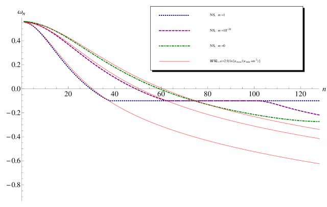
Figure 8: Dependence of the eigenvalues on the number of zeros of the eigenfunction. The dashed lines describe the numerical solution for $\omega_{n}$ for the massive BFKL equation with mass $m$. $m=0$ corresponds to massless BFKL. The orange solid curves show the values of $\omega_{n}$ calculated using Eq. (3.61) .

For massive BFKL situation is different. A simple parametrization Eq. (3.61) with nonzero $m$ may be used with a good precision only for $\omega\geq\omega_{0}$. The point $\omega\approx\omega_{0}$ is special and will be discussed in more detail below. For very large $n$ the values of the intercepts become smaller than $\omega_{0}$ and agree with Eq. (3.61), but the $n$-dependence of $\beta_{n}$ is no longer linear and will be discussed in the following section.

3.5.1.2 Eigenfunctions and Green’s function.

Eigenfunctions with $\omega\,\,\geq\,\,\omega_{0}$ first three (unnormalized) eigenfunctions corresponding to massless and massive BFKL are shown in Fig. 9. As we can see, for large $\kappa$ solutions of these equations coincide, however for $\kappa\,\lesssim 1\,$ they are different: the massless solution grows roughly as power of momenta, $\kappa^{-\gamma}$, whereas the solution in the massive case is regular and reaches a constant. One can see that $\psi_{2}\left(\kappa\right)$ has one zero while $\psi_{3}\left(\kappa\right)$ has two zeroes. This behaviour of the wave functions has been expected from the general analysis of the solution ( see subsection 1 of this section).

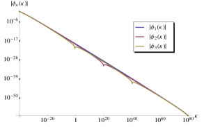
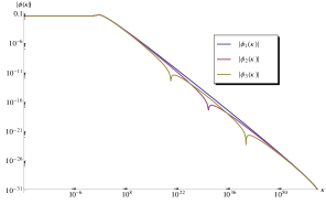
Fig. 9-a		Fig. 9-b

Figure 9: Absolute values of the first three eigenfunctions $\left|\psi_{n}\left(k\right)\right|$ corresponding to massless BFKL(Fig. 9-a) and BFKL with mass(Fig. 9-b). In the figure $k^{2}\,=\,\kappa$.

With a good precision the eigenfunctions with the eigenvalues larger than $\omega_{0}$ can be parameterized as

$$\phi^{(approx)}_{n}\left(\kappa\right)\,\,=\,\,\frac{\alpha\left(n\right)}{\sqrt{\kappa+4}}\sin\Big{(}\beta_{n}\left(m=1\right)\,Ln\left(\kappa\right)+\varphi_{n}\Big{)}~{}~{}~{}~{}~{}~{}\mbox{with}~{}~{}~{}Ln\left(\kappa\right)\,=\,\ln\Big{(}\frac{\sqrt{\kappa\,+\,4}\,\,+\,\,\sqrt{\kappa}}{\sqrt{\kappa\,+\,4}\,\,-\,\,\sqrt{\kappa}}\Big{)}$$ (3.62)

The form of the parameterization in Eq. (3.62) is inspired by the expression for the gluon trajectory $\omega(\kappa)$.

For $\kappa\ll 1$ and for $\kappa\gg 1$ the function (3.62) has an asymptotic form

$$\phi^{(approx)}_{n}\left(\kappa\right)\,\,=\,\,\left\{\begin{array}[]{l}\,\,\,\frac{1}{2}\alpha\left(n\right)\sin\left(\varphi_{n}\right)\,\,\,\,\,\mbox{for}\,\,\,\kappa\,\ll\,1\,,\\ \\ \,\,\,\frac{\alpha\left(n\right)}{\sqrt{\kappa}}\sin\left(\beta_{n}\left(m=1\right)\ln\kappa\,+\,\varphi_{n}\right)\,\,\,\,\,\mbox{for}\,\,\,\kappa\,\gg\,1\,.\end{array}\right.$$ (3.66)

Since in the large-$\kappa$ regime the massive BFKL coincides with massless BFKL, for which the second line of Eq. (3.66) is an exact solution, the parameters $\beta_{n}$ and $\varphi_{n}$ are defined for all possible values of $n$. For the case $m=1$ the dependence of $\beta_{n}$ and $\varphi_{n}$ on the number $n$ is shown in the Fig. 10. We can see that in the small-$n$ region both $\beta_{n}$ and $\varphi_{n}$ are linear functions of $n$, $\beta_{n}(m)\,=\,a(m)n$ and $\varphi_{n}\,=\,a_{\varphi}(m)n$, where $a(m)$ is given by Eq. (3.61), and

$$a_{\varphi}(m) \approx\frac{8.577\,}{\ln\left(\kappa_{max}/\kappa_{min}\right)}=b_{\varphi}\beta_{n}(m),$$ (3.67)

$$b_{\varphi} \approx 1.865,$$ (3.68)

so in this regime we may rewrite Eq. (3.62) in a form

$$\phi^{(approx)}\left(\kappa,\beta\right)\,\,=\,\,\frac{\alpha\left(\beta\right)}{\sqrt{\kappa+4}}\sin\Big{(}\beta\,Ln\left(\kappa\right)+b_{\varphi}\,\beta\Big{)}$$ (3.69)

which does not depend on lattice parameters. However, a linear approximation for $n$-dependence of $\phi_{n}$ is valid only for very small $n$. In the vicinity of the point $\omega=\omega_{0}$ both parameters freeze, and we’ll discuss this regime in more detail in the next section. For very large $n$, the intercept $\omega$ goes below $\omega_{0}$ and the parameters $\beta$, $\varphi$ resume their dependence on $n$ (see e.g. Fig. 11), however in this regime the oscillation period becomes comparable with period of the lattice, so extracted parameters are not very reliable. The normalization factor $\alpha(n)$ can be found from the normalization condition of Eq. (3.22) and is irrelevant for purposes of this paper since we are solving the linear equation.

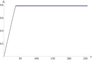
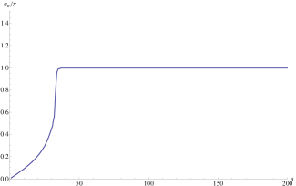
Figure 10: Left: Dependence of the eigenfuncton parameter $\beta_{n}$ on eigenfunction number $n$. Right: Dependence of the eigenfuncton parameter $\varphi_{n}$ on eigenfunction number $n$. In a chosen lattice $\omega=\omega_{0}\equiv-\frac{1}{2}\bar{\alpha}_{S}$ corresponds to $n=37$.

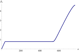
Figure 11: Large-$n$ dependence of the eigenfunction parameter $\beta$ on the eigenfunction number $n$

In order to demonstrate the quality of the fit (3.62), in the left pane of the Fig. 12 we directly compare the numerical eigefunction and parametrization (3.62). In the right pane of the Fig. 12 we plot the ratio

$$\omega^{approx}\,\,=\,\,\frac{\mbox{r.h.s.}\left(\phi^{(approx)}\left(\kappa,\beta\right)\right)}{\phi^{(approx)}\left(\kappa,\beta\right)}$$ (3.70)

which demonstrates that the deviations of the fit from numerical solution are the largest in the region $\kappa\sim 1$, however even there don’t exceed 10%.

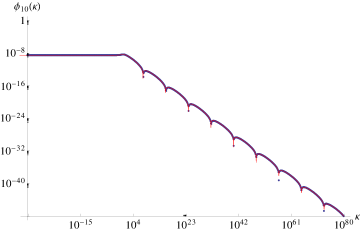
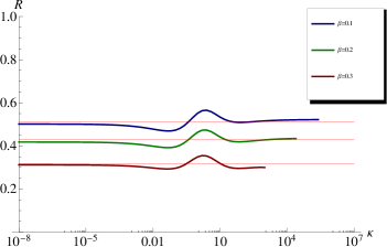
Figure 12: Left: Comparison of the approximate parametrization (3.62) (in red) with numerical result (blue) for $n=10$. Right: Check of accuracy of $\phi^{(approx)}\left(\kappa,\beta\right)$. $\omega^{approx}$ given by Eq. (3.70) (see wavy lines) and $\omega^{exact}$ (orange straight lines) at different values of $\beta$.

Eigenfunctions in the vicinity of $\omega\,\,=\,\omega_{0}$

As was discussed in previous sections, the point $\omega=\omega_{0}$ is special. We would like to investigate the behaviour near this point both analytically and numerically. The equation of motion Eq. (2.12) for $\omega\approx\omega_{0}$, or $E=\frac{1}{2}$ in the small-$\kappa$ regime has a form

$$\Big{(}E-\frac{1}{2}-\frac{5}{12}\,\kappa\Big{)}\phi\left(\kappa\right)\,\,=\,\,-\frac{N^{2}_{c}-1}{2N^{2}_{c}}\int\frac{d\kappa^{\prime}}{k^{\prime}+1}\,\phi\left(\kappa^{\prime}\right)+\mathcal{O}\left(\kappa^{2}\right)$$ (3.71)

Introducing a new notation $\epsilon=\frac{12}{5}\left(E-\frac{1}{2}\right)$ one can see that function $\phi\left(\kappa\right)$ should have a pole at $\kappa=\epsilon$,

$$\phi\left(\kappa\right)|_{\kappa\to\epsilon\ll 1}\,\,=\,\,\frac{\rm const}{\epsilon\,-\,\kappa}.$$ (3.72)

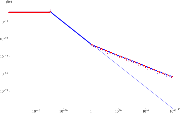
Figure 13: The eigenfunction $|\phi(\omega_{0},\kappa)|$ with $\omega=\omega_{0}\,=\,-\frac{1}{2}\bar{\alpha}_{S}$. Red curve corresponds to the positive values of $\phi(\omega_{0},\kappa)$ while blue describes the negative $\phi(\omega_{0},\kappa)$. The approximate function $|\phi^{approx}(\omega_{0},\kappa)|=|1/\left(\kappa\,-\,\kappa_{0}\right)|$ with $\kappa_{0}=10^{-30}$, is shown by the thin line. We multiply the fit result ($\phi^{approx}$) by some constant to see the difference (otherwise they just coincide).

A numerical calculation confirms our expectation. As one can see from Fig. 13, the wave function indeed has a pole at $\kappa\ll 1$. Position of the pole is arbitrary and may coincide with any node at $\kappa\ll 1$. Due to large number of nodes with $\kappa_{n}\ll 1$, the spectrum Fig. 8 looks multiply degenerate at the point $\omega=\omega_{0}$. In order to demonstrate that this is not the case, we recalculated the eigenvalues in the lattice which has a linear step in the region $\kappa\leq 1$ and a logarithmic step for $\kappa\geq 1$,

$$\kappa_{n}=\,\,\left\{\begin{array}[]{l}\,\,\,\,\frac{n}{N_{<}}~{}~{}\mbox{with}\,\,n=0,\dots,N_{<}~{}~{}~{}N_{<}=200~{}~{}~{}\mbox{for}~{}~{}\kappa\,<\,1;\\ \\ \,\,\,\,\exp\left(\frac{n}{N_{>}}\ln\kappa_{max}\right)~{}~{}\mbox{with}\,\,n=0,\dots,N_{>}\,\,\,,\,N_{>}=1024,\kappa_{max}=10^{60},~{}~{}~{}\mbox{for}\,\,\,\kappa\,>\,1\,.\end{array}\right.$$ (3.76)

From the Fig. 14 we may see that the spectrum in this case is no longer degenerate. This happens because the typical node values $\kappa_{n}\sim 10^{-2}...10^{-1}$ are much larger than with logarithmic grid and a deviation $\omega-\omega_{0}\sim\kappa_{n}$ is also larger.

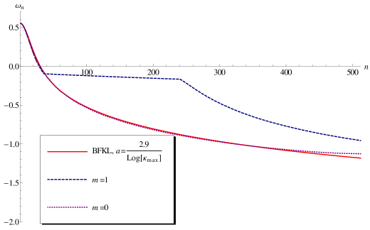
Figure 14: The eigenvalues of the massless and massive BFKL equation in the linear-logarithmic discretization (see Eq. (3.76)).The dashed lines describe the numerical solution for $\omega_{n}$ for the massive BFKL equation with mass $m$. $m=0$ corresponds to massless BFKL. The orange solid curves show the values of $\omega_{n}$ calculated using Eq. (3.61)

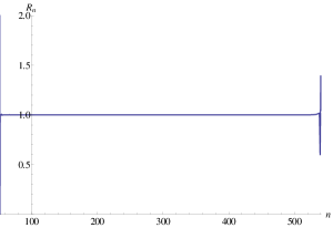
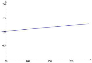
Fig. 15-a		Fig. 15-b

Figure 15: The ratio $R=\bar{\alpha}_{S}\left(5/12\right)\kappa_{0}(n)/\left(\omega(n)-\omega_{0}\right)$ versus $n$. Fig. 15-a shows this ratio in logarithmic discretization (see Eq. (3.57), while in Fig. 15-b the ratio is plotted in linear-logarithmic discretization (see Eq. (3.76) for the description)

In the Fig. 15 we demonstrate that the deviation $\omega(n)-\omega_{0}$ is proportional to the pole position $\kappa_{0}(n)$ and in agreement with Eq. (3.71) the ratio

$$R=\frac{5\bar{\alpha}_{S}}{12}\frac{\kappa_{0}(n)}{\omega_{0}(n)-\omega_{0}}$$

is close to 1 for $\omega_{0}(n)\approx\omega_{0}$. In the left pane, we have shown results with logarithmic grid, and in the right pane with grid Eq. (3.76). In the latter case, while results are close to one, there are some deviations due to $\mathcal{O}(\kappa^{2})$ terms omitted in Eq. (3.71).

For $\kappa>1$, all the wave function in the vicinity $\omega\approx\omega_{0}$ have a form given by Eq. (3.66) but with fixed $\beta_{n}=\beta^{0}=0.786$ found from $\omega(\beta^{0},m=1)=-\frac{1}{2}\bar{\alpha}_{S}$, where $\omega(\beta^{0},m=1)$ is given in Eq. (3.61).

In summary, the wave functions with $\omega\approx\omega_{0}$ may be parametrized as

$$\phi^{(approx)}_{n}\left(\kappa\right)\,\,=\,\,\left\{\begin{array}[]{l}\,\,\,\alpha\left(n\right)\,\sin\varphi_{n}\left(1-\kappa_{0}(n)\right)/(\kappa-\kappa_{0}(n))\,\,\,\,\,\mbox{for}\,\,\,\kappa\,\leq\,1\,;\\ \\ \,\,\,\frac{\alpha\left(n\right)}{\sqrt{\kappa}}\sin\left(\beta^{0}\,\ln\kappa\,+\,\varphi_{n}\right)\,\,\,\,\,\mbox{for}\,\,\,\kappa\,>\,1\,;\end{array}\right.$$ (3.80)

It is instructive to notice that Eq. (3.80) corresponds to the energy spectrum which almost does not depend on $n$ for large range of $n$ independently of the type of discretization. This fact reflects in our calculation procedure the difference of the continuous spectrum between $\omega\,>\,\omega_{0}$ and $\omega\,<\,\omega_{0}$. The former is discreet with the cut at large $\kappa$ while the latter remains continuous with this cut.

Eigenfunctions with $\omega\,\,<\,\,\omega_{0}$

For large $n$ ( $n>550$ see Fig. 8 and Fig. 14) $\omega_{n}$ become smaller than $\omega_{0}$. In this kinematic region the eigenfunction can be described by general formulae of Eq. (3.62) with $\beta$ that increases linearly with $n$ (see Fig. 11) but we need to add to this eigenfunction the term $\propto 1/(\kappa-\kappa_{0}(n))$ with $\kappa_{0}(n)\,>\,1$. However, the difference $\Delta\kappa(n)=\kappa_{0}(n+1)-\kappa_{0}(n)$ turns out to be larger than $\Delta E\left(\beta(n)\right)=E\left(\beta(n+1)\right)-E\left(\beta(n)\right)$ of Eq. (3.53) for our discretization procedure. The appearance of $1/(\kappa-\kappa_{0}(n))$ in the eigenfunction is the consequence of the fact that the spectrum remains continuous with the cut at large $\kappa$.

Note that evaluations in this region should be taken with due care because of possible interplay of oscillation period with period of the grid. The maximal value of $\beta$ which may be extracted with this method is controlled by the grid step and is given by $\beta_{max}=N/log(\kappa_{max}/\kappa_{min})~{}=\,3.7$ (see Eq. (3.57) for values of $N$, $\kappa_{max}$ and $\kappa_{min}$).

Green’s function

We can calculate the Green function of the massive BFKL Pomeron using Eq. (3.66). Indeed, the Green function takes the general form

$$G\left(Y,\kappa_{fin}|0,\kappa_{in}\right)\,\,=\,\,\sum_{n=0}^{\infty}\phi_{n}\left(\kappa_{fin}\right)\,\phi_{n}\left(\kappa_{in}\right)\,e^{\omega\left(n\right)Y}$$ (3.81)

where functions $\phi_{n}$ should be normalized according to Eq. (3.22) In the diffusion approximation we can expand the eigenvalues of Eq. (3.61) at small $n$ replacing Eq. (3.61) by the simple expression

$$\omega\left(n\right)\,\,=\,\,\omega_{\mbox{\tiny BFKL}}\,\,-\,\,D\,a^{2}\,n^{2}\,\,+\,\,{\cal O}\left(n^{3}\right)\,\,=\,\,\omega_{\mbox{\tiny BFKL}}\,\,-\,\,D\,\beta^{2}$$ (3.82)

where $\omega_{\mbox{\tiny BFKL}}\,=\,4\,\ln 2\,\bar{\alpha}_{S}$; $D\,=\,14\,\zeta(3)\,\bar{\alpha}_{S}$.

Therefore in this approximation the Green function takes the form

$$G\left(Y,\kappa_{fin}|0,\kappa_{in}\right)\,\, = \,\,e^{\omega_{\mbox{\tiny BFKL}}\,Y}\,\sum_{n=0}^{\infty}\phi_{n}\left(\kappa_{in},\beta\right)\,\phi_{n}\left(\kappa_{fin},\beta\right)\,e^{-D\,Y\,a^{2}\,n^{2}}$$ (3.83)

$$\to \,\,e^{\omega_{\mbox{\tiny BFKL}}\,Y}\,\int^{\infty}_{0}\,d\beta\,\phi_{0}\left(\kappa_{in},\beta\right)\,\phi_{0}\left(\kappa_{fin},\beta\right)\,e^{-D\,Y\,\beta^{2}}$$

The main contribution proportional to $e^{\omega_{\mbox{\tiny BFKL}}\,Y}$ stems from small $\beta$’s where we can use Eq. (3.82). Taking the integral over $\beta$ in Eq. (3.83) we obtain the following Green’s function at large values of $Y$:

$$G\left(Y,\kappa_{fin}|0,\kappa_{in}\right)\,\,=$$ (3.84)

$$\,\,\,\,\frac{1}{\sqrt{\left(\kappa_{fin}\,+\,4\right)\,\left(\kappa_{in}+4\right)}}\,\frac{1}{2}\,e^{\omega_{\mbox{\tiny BFKL}}Y}\,\sqrt{\frac{\pi}{D\,Y}}\Bigg{\{}e^{-\frac{\left(L\left(\kappa_{fin}\right)\,-\,L\left(\kappa_{in}\right)\right)^{2}}{4\,D\,a^{2}\,Y}}\,\,-\,\,e^{-\frac{\left(L\left(\kappa_{fin}\right)\,+\,L\left(\kappa_{in}\right)\,\,+\,\,2\,b_{\phi}\right)^{2}}{4\,D\,a^{2}\,Y}}\Bigg{\}}$$

One can see that at large $Y$ Green function $G\left(Y,\kappa_{fin}|0,\kappa_{in}\right)\,\,\propto\,\,\left(D\,Y\right)^{-3/2}\,e^{\omega_{\mbox{\tiny BFKL}}Y}$, which should be compared with the massless BFKL case for which $G\left(Y,\kappa_{fin}|0,\kappa_{in}\right)\,\,\propto\,\,\left(D\,Y\right)^{-1/2}\,e^{\omega_{\mbox{\tiny BFKL}}Y}$. It is related to the fact, that in the massive case the diffusion approximation is valid only at large positive $\kappa$ with a boundary condition at fixed $\kappa$.

3.5.2 Evolution method

In this method the leading $\omega$ - plane singularity is extracted using an evolution in rapidity $Y$,

$$\frac{\partial\Psi}{\partial Y}\,\,=\,\,\bar{\alpha}_{S}\,\int d^{2}k^{\prime}\,K\left(k,k^{\prime}\right)\Psi\left(k^{\prime},Y\right),$$ (3.85)

where

$$\Psi\left(k,Y\right)\,\,=\,\,\int^{\epsilon+i\infty}_{\epsilon-i\infty}\frac{d\omega}{2\pi i}e^{\omega Y}\,\phi_{\omega}\left(\kappa\right),$$ (3.86)

and $\kappa\,=\,k^{2}$.

For asymptotically large $Y$ at any initial condition function $\Psi\left(Y_{0},k\right)$ may be decomposed over the eigenfunctions of the hamiltonian $\mathcal{H}$,

$$\Psi(Y,k)\,\,=\,\,\sum_{n}c_{n}\,\phi_{n}(k)\,e^{\omega_{n}Y},$$ (3.87)

As has been mentioned the spectrum is discrete since on the grid we always have a cutoff at large $k_{T}$. From naive counting for asymptotically large $Y$ we have

$$\Psi(Y,k) \sim c_{0}\phi_{0}(k)\,e^{\omega_{0}Y}\,\left(1+\frac{c_{1}}{c_{0}}e^{-\Delta\omega Y}\right),$$

$$\Delta\omega =\omega_{0}-\omega_{1}>0$$

however in reality the situation is more complicated since we have inhomogeneous convergence and the limits don’t commute

$$\lim_{k_{max}\to\infty}\Delta\omega\,\,=\,\,0,~{}~{}~{}~{}~{}~{}~{}~{}~{}~{}~{}~{}~{}~{}\lim_{k_{max}\to\infty,Y\to\infty}\Delta\omega\,Y\,\,=\,\,0\cdot\infty={\rm undefined}$$ (3.88)

In the case of massless BFKL equation the summation over $n$ in Eq. (3.87) leads to the asymptotic behaviour at high energy which has been discussed after Eq. (3.84).

For evolution we used a modified BK code [20] with default conditions, $\ln\,k_{min}^{2}\in(-20,\,138)$ and $N=1024$ points in logarithmic grid. The corresponding leading eigenvalues extracted with this method are $\omega_{0}\,=\,0.545$ for massless case and $\omega_{0}\,=\,0.537$ for the massive case. The results of the wave function are shown in Fig. 16-a . In Fig. 16-b we compare these wave functions with those extracted with direct method. For the massive case we see that both function are almost identical. For massless equation we can see that in both cases the qualitative behavior is very similar, though quantitatively the curves differ at large $k_{T}$. Since the wave function is suppressed there by a few orders of magnitude, we believe that this uncertainty should not affect the physical observables.

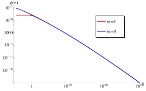
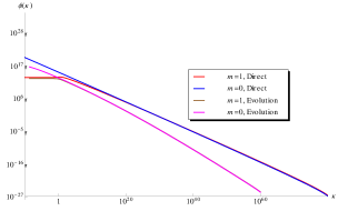
Fig. 16-a		Fig. 16-b

Figure 16: Leading eigenfunctions for the massive and massless BFKL equation extracted with evolution method (Fig. 16-a ). Comparison of leading eigenfunctions extracted with direct method and evolution (Fig. 16-b). Note that the eigenfunctions extracted in both methods have different normalization, so for comparison we have multiplied the direct solution by a normalization factor to match massive BFKL with both methods at $k=1$.

4 BFKL equation with mass at $q\neq 0$.

4.1 Large impact parameter dependence

The kernel of the BFKL equation at $q\neq 0$ is given by Eq. (2) which we re-write using more symmetric notations for gluon momenta

$$\vec{q}_{1}\,=\,\frac{1}{2}\vec{q}\,+\,\vec{p}\,;\,\,\,\,\,\vec{q}_{2}\,=\,\frac{1}{2}\vec{q}\,-\,\vec{p}\,;\,\,\,\,\,\vec{q}\,^{\prime}_{1}=\frac{1}{2}\vec{q}+\vec{p}\,^{\prime}\,\,\,\,\,\vec{q}^{\,\,{}^{\prime}}_{2}\,=\,\frac{1}{2}\vec{q}\,-\,\vec{p}^{\,\,{}^{\prime}}\,;\,\,\,\,\,\vec{k}\,=\,\vec{p}\,-\,\vec{p}^{\,\,{}^{\prime}}\,$$ (4.89)

It takes the form

$$K\left(\vec{q},\vec{p},\vec{p}^{\,{}^{\prime}}\right)\,\,=$$ (4.90)

$$\,\,\frac{\bar{\alpha}_{S}}{2\pi}\left\{\overbrace{\frac{1}{k^{2}+m^{2}}\,\left(\frac{\left(\frac{1}{2}\vec{q}+\vec{p}\right)^{2}+m^{2}}{\left(\frac{1}{2}\vec{q}+\vec{p}^{\,\,{}^{\prime}}\right)^{2}+m^{2}}\,\,+\,\,\frac{\left(\frac{1}{2}\vec{q}-\vec{p}\right)^{2}+m^{2}}{\left(\frac{1}{2}\vec{q}-\vec{p}^{\,\,{}^{\prime}}\right)^{2}+m^{2}}\right)}^{\rm emission\,\,\,\,kernel:\,K_{em}\left(\vec{q},\vec{p},\vec{p}^{\,{}^{\prime}}\right)}\,\,-\,\,\underbrace{\frac{q^{2}+\frac{N^{2}_{c}+1}{N^{2}_{c}}\,m^{2}}{\left(\,\left(\frac{1}{2}\vec{q}+\vec{p}^{\,\,{}^{\prime}}\right)^{2}+m^{2}\right)\,\left(\,\left(\frac{1}{2}\vec{q}-\vec{p}^{\,\,{}^{\prime}}\right)^{2}+m^{2}\right)}}_{\rm contact\,\,\,\,\,\,\,term:\,\,K_{ct}\left(\vec{q},\vec{p}^{\,{}^{\prime}}\right)}\right\}$$

First, we re-write this kernel in the impact parameter representation using the following formulae:

$$K\left(\vec{b},\vec{p},\vec{p}^{\,\,{}^{\prime}}\right)\,\,=\,\,\int d^{2}qe^{i\vec{q}\cdot\vec{b}}\,K\left(\vec{q},\vec{p},\vec{p}^{\,{}^{\prime}}\right)$$ (4.91)

$$\int d^{2}qe^{i\vec{q}\cdot\vec{b}}\frac{\left(\frac{1}{2}\vec{q}+\vec{p}\right)^{2}+m^{2}}{\left(\frac{1}{2}\vec{q}+\vec{p}^{\,\,{}^{\prime}}\right)^{2}+m^{2}}\,=\,e^{2i\vec{p}\cdot\vec{b}}\Big{(}-\frac{1}{4}\nabla^{2}_{b}+m^{2}\Big{)}4\int d^{2}le^{i\vec{l}\cdot\vec{b}}\frac{1}{(\vec{l}+\vec{k})^{2}+m^{2}}\,\,$$

$$=\,\,4\,e^{2i\vec{p}\cdot\vec{b}}\Big{(}-\frac{1}{4}\nabla^{2}_{b}+m^{2}\Big{)}e^{2i\vec{k}\cdot\vec{b}}\,K_{0}\left(2mb\right)\,=\,e^{2i\vec{p}^{\,\,{}^{\prime}}\cdot\vec{b}}\,\left\{k^{2}K_{0}\left(2mb\right)\,\,+\,\,2im\frac{\vec{k}\cdot\vec{b}}{b}\,K_{1}\left(2mb\right)\right\}$$

where $K_{i}(z)$ are the modified Bessel functions of the second kind.

Using Eq. (4.1) we can re-write the first two terms of Eq. (4.90) (emission kernel $K_{em}\left(\vec{q},\vec{p},\vec{p}^{\,{}^{\prime}}\right)$) in the following form

$$K_{em}\left(\vec{b},\vec{p},\vec{p}^{\,{}^{\prime}}\right)\,\,=\,\,\bar{\alpha}_{S}\left(\frac{k^{2}}{k^{2}+m^{2}}\cos\left(2\vec{p}^{\,\,{}^{\prime}}\cdot\vec{b}\right)\,\,K_{0}\left(2mb\right)\,\,\,+\,\,2m\frac{\vec{k}\cdot\vec{b}}{b}\sin\left(2\vec{p}^{\,\,{}^{\prime}}\cdot\vec{b}\right)\,\,K_{1}\left(2mb\right)\right)$$ (4.93)

In the contact term of Eq. (4.90) we can replace $\vec{q}^{\,\,{}^{\prime}}_{2}\,=\,\frac{1}{2}\vec{q}\,-\,\vec{p}^{\,\,{}^{\prime}}$ and obtain the following expression

$$K_{ct}\left(\vec{b},\vec{q}^{\,{}^{\prime}}_{2}\right)\,\, = \,\,\frac{\bar{\alpha}_{S}}{q^{\prime 2}_{2}+m^{2}}\left(-\nabla^{2}_{b}+\frac{N^{2}_{c}+1}{N^{2}_{c}}\,m^{2}\right)\,e^{\vec{q}^{\,\,{}^{\prime}}_{2}\cdot\vec{b}}\,K_{0}\left(mb\right)$$

$$= \,\frac{\bar{\alpha}_{S}}{q^{\prime 2}_{2}+m^{2}}e^{i\vec{q}^{\,\,{}^{\prime}}_{2}\cdot\vec{b}}\left(q^{\prime 2}_{2}K_{0}\left(mb\right)\,\,+\frac{m^{2}}{N^{2}_{c}}K_{0}\left(mb\right)\,+\,2im\frac{\vec{q}^{\,\,{}^{\prime}}_{2}\cdot\vec{b}}{b}\,K_{1}\left(mb\right)\right)$$

It is worthwhile mentioning that we can replace $\vec{q}_{2}^{\,\,{}^{\prime}}$ by $\vec{p}^{\,\,{}^{\prime}}$ in this part of the kernel since we have the integration over $q^{\prime}_{2}$.

The part of the BFKL kernel that is responsible for the gluon reggeization for $q\neq 0$ takes the following form (see Eq. (2.8), Eq. (2.9) and Eq. (4.89))

$$K_{reg}\left(\vec{q},\vec{p}\right)\,\,=\,\,\omega\left(|\frac{1}{2}\vec{q}+\vec{p}\,|\right)\,\,+\,\,\omega\left(|\frac{1}{2}\vec{q}-\vec{p}\,|\right)$$ (4.95)

Using Eq. (2.9) and Eq. (4.1) $K_{reg}\left(\vec{q},\vec{p}\right)$ in $b$ representation takes the form:

$$K_{reg}\left(\vec{b},\vec{p}\right)\,\,=\,\,\bar{\alpha}_{S}\,m^{2}\cos\left(2\,\vec{p}\cdot\vec{b}\right)\,\Big{\{}K^{2}_{0}\left(2mb\right)\,\,+\,\,2K^{2}_{1}\left(2mb\right)\Big{\}}$$ (4.96)

Finally, the entire kernel in $b$ representation looks as follows

$${\cal K}\left(\vec{b},\vec{p},\vec{p}^{\,\,{}^{\prime}}\right)\,\,=\,\,K_{em}\left(\vec{b},\vec{p},\vec{p}^{\,\,{}^{\prime}}\right)\,\,+\,\,K_{ct}\left(\vec{b},\vec{p}^{\,\,{}^{\prime}}\right)\,\,+\,\,K_{reg}\left(\vec{b},\vec{p}\right)\,\delta^{(2)}\left(\vec{p}\,-\,\vec{p}^{\,\,{}^{\prime}}\right)$$ (4.97)

and the massive BFKL equation takes the form

$$\frac{\partial f\left(\vec{b},\vec{p}\,|Y\right)}{\partial Y}\,\,=\,\,\int d^{2}b^{\prime}\,d^{2}p^{\prime}\,{\cal K}\left(\vec{b}^{\,\,{}^{\prime}},\vec{p},\vec{p}^{\,\,{}^{\prime}}\right)\,f\left(\vec{b}\,-\,\vec{b}^{\,\,{}^{\prime}},\vec{p}^{\,\,{}^{\prime}}|Y\right)$$ (4.98)

At large $b\,\gg\,m$ kernel ${\cal K}$ falls down exponentially, namely K$\,\propto\exp\left(-\,m\,b\right)$ which leads to $f\left(\vec{b},\vec{p}\,|Y\right)\,\,\propto\,\exp\left(-\,m\,b\right)$. Indeed, assuming that $b^{\prime}\sim 1/m$ contribute to the integral over $b^{\prime}$ in Eq. (4.98), we can re-write this equation in the form

$$\frac{\partial f\left(\vec{b},\vec{p}\,|Y\right)}{\partial Y}\,\,=$$ (4.99)

$$\,\,\int\,d^{2}p^{\prime}\,\left\{\int d^{2}b^{\prime}{\cal K}\left(\vec{b}^{\,\,{}^{\prime}},\vec{p},\vec{p}^{\,\,{}^{\prime}}\right)\,\right\}f\left(\vec{b},\vec{p}^{\,\,{}^{\prime}}|Y\right)\,\,+\,\,\int\,d^{2}p^{\prime}\,{\cal K}\left(\vec{b},\vec{p},\vec{p}^{\,\,{}^{\prime}}\right)\,\left\{\int d^{2}b^{\prime}f\left(\vec{b}^{\,\,{}^{\prime}},\vec{p}^{\,\,{}^{\prime}}|Y\right)\right\}$$

Noticing that the largest asymptotic behaviour at large $b$ stems from $K_{ct}$ we can re-write Eq. (4.99) in the form:

$$\frac{\partial f\left(\vec{b},\vec{p}\,|Y\right)}{\partial Y}\,\,=$$ (4.100)

$$\,\,\int\,d^{2}p^{\prime}\,\left\{\int d^{2}b^{\prime}{\cal K}\left(\vec{b}^{\,\,{}^{\prime}},\vec{p},\vec{p}^{\,\,{}^{\prime}}\right)\,\right\}f\left(\vec{b},\vec{p}^{\,\,{}^{\prime}}|Y\right)\,\,+\,\,\bar{\alpha}_{S}\,e^{-mb}\int\,d^{2}p^{\prime}\frac{J_{0}\left(p^{\prime}b\right)}{p^{\prime 2}+m^{2}}\,\underbrace{\left\{\int d^{2}b^{\prime}f\left(\vec{b}^{\,\,{}^{\prime}},\vec{p}^{\,\,{}^{\prime}}|Y\right)\right\}}_{\rm solution\,\,at\,\,\,q^{2}=0}$$

As we have discussed, our solution at $q^{2}=0$ behaves as $\left(p^{2}\right)^{-\frac{1}{2}+i\nu}$ at large $p$ but it is constant at $p\to 0$. Integral over $p^{\prime}$ in the non-homogeneous term in Eq. (4.100) is concentrated at small values of $p^{\prime}\sim 1/b\leq m$ leading only to mild power-like dependence on $b$. Therefore, searching solution in the form: $f\left(\vec{b},\vec{p}\,|Y\right)\,=\,\exp\left(-m\,b\right)\tilde{f}\left(\vec{b},\vec{p}\,|Y\right)$ we see that for $\tilde{f}\left(\vec{b},\vec{p}\,|Y\right)$ we obtain an equation with the non-homogeneous term that only weakly (power-like) falls at large $b$.

Hence we can conclude that at large impact parameters the solution to the BFKL equation with mass falls down as $\exp\left(-m\,b\right)$ as it was expected.

4.2 Equation for $\langle|b^{2}|\rangle$

In this section we are going to derive the equation that will allow us to calculate $\langle|b^{2}|\rangle$ as a function of $Y$. In the parton model this observable is proportional to the number of emissions due to Gribov’s diffusion[21] which is sketched in Fig. 17.

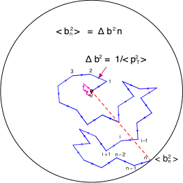
Figure 17: Gribov’s diffusion for emissions in the parton model (blue line) and in QCD (red line).

The average $b^{2}$ after $n$ emissions is equal

$$\langle|b^{2}_{n}|\rangle\,\,=\,\,\Delta b^{2}\,n\,\,=\,\,\frac{1}{\langle|p^{2}_{T}|\rangle}\,n$$ (4.101)

Since the average number of emissions at given $Y$ is proportional to $Y$ and the average $\langle|p^{2}_{T}|\rangle$ is a constant independent from $Y$ in the parton model, $\langle|b^{2}|\rangle\,\,=\,\,4\,\alpha^{\prime}_{I\!\!P}\,Y$ where $\alpha^{\prime}_{I\!\!P}$ is the slope of the Pomeron trajectory. In QCD the average transverse momentum increases with energy $Y$. We plot in Fig. 18 the contours on which function $k\,\Psi\left(k,Y\right)$ (see Eq. (3.85)) is constant. One can see that for the massive BFKL equation the average $p_{T}$ are larger than the values of $p_{T}$ in initial conditions and they grow with $Y$. One can see from Eq. (4.101) that $\Delta b^{2}$ decreases at large $Y$ leading to $\langle|b^{2}_{n}|\rangle\,\xrightarrow{\mbox{ $Y\,\,\gg\,\,1$}}\,0$ since $\langle|p^{2}_{T}|\rangle$ increases faster than $Y$ ( see Fig. 18). Therefore, we expect that in QCD $\langle|b^{2}|\rangle$ for the massive BFKL Pomeron does not depend on $Y$ repeating the main features of the massless BFKL Pomeron.

We would like to stress that this discussion is based on the uncertainty principle $\Delta p_{T}\Delta b\sim 1$. Fig. 18 shows that if we replace in Eq. (4.101) $1/\langle|p^{2}_{T}|\rangle$ by $\langle|1/p^{2}_{T}|\rangle$ we can expect that massive BFKL equation will lead to Gribov’s diffusion since $\langle|1/p^{2}_{T}|\rangle\propto 1/m^{2}$. Therefore, we need to calculate $\langle|b^{2}|\rangle$ for massive BFKL Pomeron to justify the simple picture that stems from Fig. 17.

The general expression for $\langle|b^{2}|\rangle$ takes the form

$$\langle|b^{2}|\rangle\,\,=\,\,\frac{\int d^{2}b\,b^{2}\,f\left(\vec{b},\vec{p}\,|Y\right)}{\int d^{2}b\,f\left(\vec{b},\vec{p}\,|Y\right)}$$ (4.102)

and for $N\left(\vec{p}\,|Y\right)\,=\,\int d^{2}b\,b^{2}\,f\left(\vec{b},\vec{p}\,|Y\right)$ we can write the equation using the expression for the BFKL kernel in $b$ representation (see Eq. (4.97)).

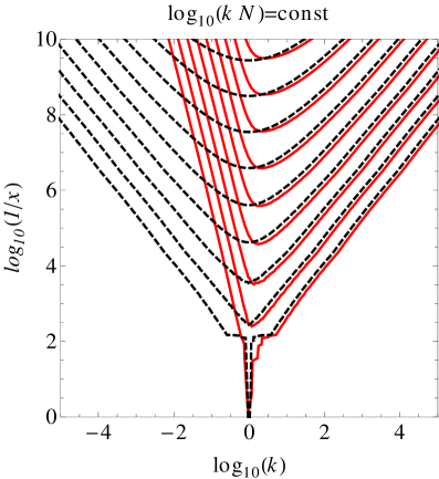
Figure 18: The contour with constant $k\Psi\left(k,Y\right)$ (see dotted line) for the massless BFKL equation and for the BFKL equation with mass (see solid red line) .

However, it turns out much simpler to derive this equation using that

$$N\left(\vec{p}\,|Y\right)\,=\,\int d^{2}b\,b^{2}\,f\left(\vec{b},\vec{p}\,|Y\right)\,=\,\int d^{2}b\int d^{2}q\left(-\nabla^{2}_{q}e^{-i\vec{q}\cdot\vec{b}}\right)\,f\left(\vec{q},\vec{p},|Y\right)\,\,=\,\,-\left(\nabla^{2}_{q}\,\Psi\left(\vec{q},\vec{p}|Y\right)\right)|_{q=0}$$ (4.103)

where $\Psi$ is defined in Eq. (3.85).

Applying operator $-\nabla^{2}_{q}$ to both parts of the evolution equation in $Y$ at $q\,\neq\,0$ we obtain

$$-\,\nabla^{2}_{q}\left\{\frac{\partial\Psi\left(\vec{q},\vec{p}|Y\right)}{\partial Y}\,\right. = \,\left.\int d^{2}p^{\prime}\,{\cal K}\left(\vec{q},\vec{p},\vec{p}^{\,\,{}^{\prime}}\right)\,\Psi\left(\vec{q},\vec{p}^{\,\,{}^{\prime}}|Y\right)\right\}$$

$$\frac{\partial N\left(\vec{p}|Y\right)}{\partial Y} = \int\!\!d^{2}p^{\prime}{\cal K}\left(q=0,\vec{p},\vec{p}^{\,\,{}^{\prime}}\right)\,N\left(\vec{p}^{\,\,{}^{\prime}}|Y\right)+\int\!\!d^{2}p^{\prime}\,\left(-\nabla^{2}_{q}{\cal K}\left(\vec{q},\vec{p},\vec{p}^{\,\,{}^{\prime}}\right)|_{q=0}\right)\Psi\left(\vec{p}^{\,\,{}^{\prime}}|Y\right)$$ (4.104)

$$+ \left\{\int d^{2}p^{\prime}\,\left(-\nabla_{q}{\cal K}\left(\vec{q},\vec{p},\vec{p}^{\,\,{}^{\prime}}\right)\right)|_{q=0}\left(\nabla_{q}\Psi\left(\vec{q},\vec{p}|Y\right)\right)|_{q=0}\right\}\,\,=\,\,0$$ (4.105)

Using the kernel of Eq. (2) and the notations of the momenta of gluons according to Eq. (4.89) we see that $\left(\nabla_{q}{\cal K}\left(\vec{q},\vec{p},\vec{p}^{\,\,{}^{\prime}}\right)\right)|_{q=0}\,=\,0$. Using Eq. (4.90) we obtain the following expression for $\left(-\nabla^{2}_{q}{\cal K}\left(\vec{q},\vec{p},\vec{p}^{\,\,{}^{\prime}}\right)\right)|_{q=0}$:

$$4{\cal K}_{1}\left(p,p^{\prime}\right)\,\equiv\,\left(-\nabla^{2}_{q}{\cal K}\left(\vec{q},\vec{p},\vec{p}^{\,\,{}^{\prime}}\right)\right)|_{q=0}\,\,=$$ (4.106)

$$\,\,\frac{2}{\,\left(p^{\prime 2}+m^{2}\right)\left(p^{2}+m^{2}\right)}\,+\,\frac{4m^{2}}{\left(p^{\prime 2}+m^{2}\right)^{2}\left((\vec{p}-\vec{p}^{{}^{\prime}})^{2}+m^{2}\right)}\,-\,\frac{4m^{2}}{2\left(p^{\prime 2}+m^{2}\right)\left(p^{2}+m^{2}\right)\left((\vec{p}-\vec{p}^{{}^{\prime}})^{2}+m^{2}\right)}.$$

Hence Eq. (4.2) gives the equation for $N\left(\vec{p}|Y\right)$.

$$\frac{\partial N\left(\kappa|Y\right)}{\partial\bar{\alpha}_{S}Y}\,=$$ (4.107)

$$\,\,\frac{\kappa+1}{\sqrt{\kappa}\sqrt{\kappa+4}}\ln\frac{\sqrt{\kappa+4}+\sqrt{\kappa}}{\sqrt{\kappa+4}-\sqrt{\kappa}}N\left(\kappa|Y\right)\,\,-\,\,\int^{\infty}_{0}\,\frac{d\kappa^{\prime}N\left(\kappa^{\prime}|Y\right)}{\sqrt{(\kappa-\kappa^{\prime})^{2}\,+\,2(\kappa+\kappa^{\prime})+1}}\,\,-\,\,\frac{N^{2}_{c}+1}{2N^{2}_{c}}\frac{1}{\kappa+1}\int^{\infty}_{0}\frac{N\left(\kappa^{\prime}|Y\right)\,d\kappa^{\prime}}{\kappa^{\prime}+1}$$

$$-4\int^{\infty}_{0}d\kappa^{\prime}\Bigg{\{}\frac{1}{2(\kappa^{2}+1)^{2}}\,-\,\frac{2\kappa+\kappa^{\prime}+2}{2(\kappa+1)^{2}(\kappa^{\prime}+1)\sqrt{(\kappa-\kappa^{\prime})^{2}+2(\kappa+\kappa^{\prime})+1}}\Bigg{\}}\Psi\left(\kappa^{\prime}|Y\right)$$

$$+2\Bigg{\{}\frac{\left(1-2\kappa\right)}{\kappa\left(\kappa+4\right)^{2}}\,+\,\frac{\left(4+6\kappa-\kappa^{2}\right)}{2\sqrt{\kappa}\left(\kappa+4\right)\left(\kappa+1\right)}\omega\left(\kappa\right)\Bigg{\}}\Psi\left(\kappa|Y\right)$$

Two remarks are needed: first, we substitute $N_{c}=3$ in the last two terms; and second, the last term stems from the expansion of the gluon trajectory( see Eq. (2.9)) in the master equation (see Eq. (2.8)) where their contribution takes the form: $\omega\left(\vec{p}-\vec{q}/2\right)+\omega\left(\vec{p}-\vec{q}/2\right)$.

Fig. 19 shows $\langle|b^{2}|\rangle$ of Eq. (4.102) in which we plug in the solution to Eq. (4.107). We can see two general features: $\langle|b^{2}|\rangle$ tends to a constant at large values of $Y$ in accordance with the qualitative discussion (see Fig. 17 and Fig. 18 ); and $\langle|b^{2}|\rangle$ does not depend on $\kappa$ for $\kappa_{1}<1$ and $\kappa_{2}<1$ but falls down for $\kappa\,>\,1$.

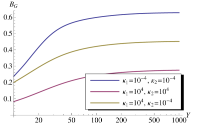
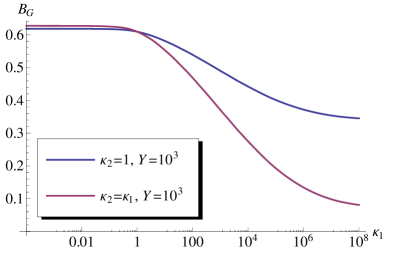
Fig. 19-a	Fig. 19-b

Figure 19: $\langle|b^{2}|\rangle$ versus $Y$ (Fig. 19-a) and $\kappa_{1}$(Fig. 19-b).

4.3 Corrections of the order of $q^{2}$

In this section we develop a systematic approach to the BFKL taking into account all corrections to the BFKL equation of the order of $q^{2}$. Such expansion is justified for all the eigenfunctions except those whose eigenvalues are in the vicinity of the point $\omega=\omega_{0}$. As one can see from Eq. (3.71), near this point there is a cancellation of two leading order terms, so the small corrections will affect position of the pole and thus cannot be treated in a perturbative approach.

Expanding the BFKL kernel of Eq. (2) we obtain

$$K =K_{0}+q^{2}K_{1},$$ (4.108)

$$K_{1} =\frac{\bar{\alpha}_{S}}{2\pi}\left[-\frac{1}{2\left(p^{\prime 2}+m^{2}\right)\left(m^{2}+p^{2}\right)}+\frac{m^{2}}{2\left((\vec{p}^{\,\,{}^{\prime}}-\vec{p})^{2}+m^{2}\right)\left(p^{\prime 2}+m^{2}\right)\left(m^{2}+p^{2}\right)}-\frac{m^{2}}{\left((\vec{p}^{\,\,{}^{\prime}}-\vec{p})^{2}+m^{2}\right)\left(p^{\prime 2}+m^{2}\right)^{2}}\right.$$

$$+\left.\frac{N_{c}^{2}+1}{N_{c}^{2}}\frac{m^{4}}{2\left(p^{\prime 2}+m^{2}\right)^{3}\left(m^{2}+p^{2}\right)}\right]+$$

$$+\frac{\bar{\alpha}_{S}}{2\pi}\delta^{(2)}(\vec{p}-\vec{p}^{\,\,{}^{\prime}})\left[\frac{m^{2}\left(m^{2}-2p^{2}\right)}{p^{2}\left(p^{2}+4m^{2}\right)^{2}}+\frac{m^{2}\left(p^{4}-6m^{2}p^{2}-4m^{4}\right)\log\left(\frac{\sqrt{p^{2}+4m^{2}}+p}{\sqrt{p^{2}+4m^{2}}-p}\right)}{2p^{3}\left(p^{2}+4m^{2}\right)^{5/2}}\right]$$ (4.109)

where $K_{0}$ is the BFKL kernel at $q=0$. Eq. (4.3) gives the emission part of the kernel, while Eq. (4.3) stems from the reggeization term of the kernel which has a general form $\omega\left(\left(\frac{1}{2}\vec{q}\,-\,\vec{p}\right)^{2}\right)\,+\,\omega\left(\left(\frac{1}{2}\vec{q}\,+\,\vec{p}\right)^{2}\right)$ (see Eq. (2.9)). Rigorously speaking at small values of $q$ the expansion has two types of corrections: the first contribution is proportional to $q^{2}$ and the second one which is proportional to $\left(\vec{p}\cdot\vec{q}\right)^{2}$. However, below we will assume that the wave function does not depend on orientation of the vector $q$ (this is correct assumption since conformal spin is zero for the ground state), so after integration (averaging) over the orientations of $\vec{p}$ we will get for such corrections $\left(\vec{p}\cdot\vec{q}\right)^{2}\,=\,\frac{1}{2}q^{2}\,p^{2}$. Deriving Eq. (4.3) we performed this averaging assuming that the wave function does not depend on the orientation of vector $q$. The fact that we do not ha ve the term of the order of $\left(\vec{p}\cdot\vec{q}\right)$ in the expansion of the BFKL kernel supports our assumption.

Considering $K_{1}q^{2}$ as perturbation we obtain the following expression for the shift of the eigenvalue of the BFKL equation

$$\left.\frac{d\omega_{n}}{dq^{2}}\right|_{q=0}=\frac{\int d\kappa_{1}d\kappa_{2}\phi_{n}\left(\kappa_{1}\right)\phi_{n}\left(\kappa_{2}\right)K_{1}\left(\kappa_{1},\kappa_{2}\right)}{\int d\kappa_{1}\left|\phi_{n}\left(\kappa_{1}\right)\right|^{2}}$$ (4.110)

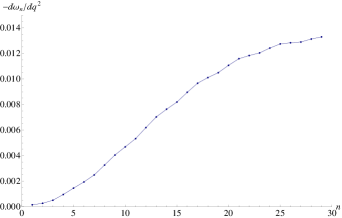
Figure 20: The shift in the eigenvalues $d\omega_{n}/dq^{2}$ due to $q^{2}$-dependence of the BFKL kernel. $n$ is the number of roots in the eigenfunctions.

$d\omega_{n}/dq^{2}$ is plotted in Fig. 20 as a function of $n$ where $n$ is the number of zeroes in the eigenfunction. One can see that at $n\,=\,0$ $d\omega_{n}/dq^{2}$ is equal to zero and at small $n$ it behaves as $d\omega_{n}/dq^{2}\,\,=\,\,a_{q}\,n^{2}$.

The corrections to the eigenfunctions look as follows:

$$\left.\frac{d\phi_{n}\left(\kappa,q\right)}{dq^{2}}\right|_{q=0}=\sum_{k\not=n}\frac{\phi_{k}(\kappa)}{\omega_{n}-\omega_{k}}\frac{\int d\kappa_{1}d\kappa_{2}\phi_{n}\left(\kappa_{1}\right)\phi_{k}\left(\kappa_{2}\right)K_{1}\left(\kappa_{1},\kappa_{2}\right)}{\int d\kappa_{1}\left|\phi_{k}\left(\kappa_{1}\right)\right|^{2}}.$$ (4.111)

Eq. (4.110) and Eq. (4.111) allows us to calculate the elastic slope of the scattering amplitude which is defined as

$$B\left(Y;k_{fin}\right)\,\,=\,\,\frac{1}{4}\,\langle b^{2}\rangle\,\,=\,\,2\,\frac{d\,\mbox{Im}A\left(Y,k_{fin}|q\right)}{d\,q^{2}}{\Big{|}}_{q=0}{\Bigg{/}}\mbox{Im}A\left(Y,k_{fin}|q=0\right)$$ (4.112)

where $A\left(Y,k_{fin}|q\right)$ is the scattering amplitude which is equal to $\Psi\left(Y,k_{fin}\right)$ of Eq. (3.87) at $q=0$. Generally speaking this observable depends on the initial condition for the scattering amplitude at $Y=0$. However, in the diffusion approximation this dependence factorizes and can be cancelled in Eq. (4.112).

Bearing this in mind we calculate $B$ for the Pomeron Green function: viz.

$$B_{G}\left(Y;k_{fin},k_{in}\right)\,\,=\,\,2\,\frac{d\,G\left(Y,k_{fin},k_{in}|q\right)}{d\,q^{2}}{\Big{|}}_{q=0}{\Bigg{/}}G\left(Y,k_{fin},k_{in}|q=0\right)$$ (4.113)

Using the general definition of the Green function, we obtain

$$G\left(Y,\kappa_{fin}|0,\kappa_{in};q\right)\,\,=\,\,\sum_{n=0}^{\infty}\phi_{n}\left(\kappa_{fin};q\right)\,\phi_{n}\left(\kappa_{fin};q\right)\,e^{\omega_{n}\left(q\right)Y}$$ (4.114)

which leads to the following expression for $B_{G}$:

$$B_{G}\left(Y;k_{fin},k_{in}\right)\,\, = \,\,\frac{2}{G\left(Y,k_{fin},k_{in}|q=0\right)}\Bigg{\{}\sum_{n=0}^{\infty}\frac{d\omega}{dq^{2}}\,Y\,\phi_{n}\left(\kappa_{fin};q=0\right)\,\phi_{n}\left(\kappa_{fin};q=0\right)\,e^{\omega_{n}\left(q=0\right)Y}\,$$

$$+ \,\sum_{n=0}^{\infty}e^{\omega_{n}\left(q=0\right)Y}\,\Big{[}\frac{d\phi_{n}\left(\kappa_{fin};q\right)}{dq^{2}}{\Big{|}}_{q=0}\,\phi_{n}\left(\kappa_{fin};q=0\right)\,\,+\,\,\phi_{n}\left(\kappa_{fin};q=0\right)\frac{d\,\phi_{n}\left(\kappa_{fin};q\right)}{dq^{2}}{\Big{|}}_{q=0}\Big{]}\Bigg{\}}$$

The first term increases with $Y$ and gives the main contribution at large values of $Y$. As one can see from Fig. 20 at small $n$ $d\omega_{n}(q)/dq^{2}\,\,=\,\,a_{q}\,n^{2}\,\,=\,\,b_{q}\,\beta^{2}$. Using this expression and the diffusion approximation of Eq. (3.82) we can obtain the simple formula for the first term in Eq. (4.3):

$$B^{(1)}_{G}\left(Y;k_{fin},k_{in}\right)\,\, = \,\,\frac{2}{G\left(Y,k_{fin},k_{in}|q=0\right)}\,\sum_{n=0}^{\infty}\frac{d\omega}{dq^{2}}\,Y\,\phi_{n}\left(\kappa_{fin};q=0\right)\,\phi_{n}\left(\kappa_{fin};q=0\right)\,e^{\omega_{n}\left(q=0\right)Y}\,\,$$ (4.116)

$$= \,\frac{2}{G\left(Y,k_{fin},k_{in}|q=0\right)}\,\int_{0}^{\infty}d\beta b_{q}\,\beta^{2}\,Y\,\phi\left(\kappa_{fin},\beta;q=0\right)\,\phi\left(\kappa_{fin},\beta;q=0\right)\,e^{\omega_{n}\left(q=0\right)Y}\,\,$$

$$= \,\,-2\,b_{q}\,\frac{d\ln G\left(Y,k_{fin},k_{in}|q=0\right)}{d\left(D\,Y\right)}$$

We can evaluate this contribution using Eq. (3.84). One can see that at large $Y$ $B^{(1)}\,\to\,(3/2)b_{q}/D$ . Therefore, Eq. (4.3) leads to $B$ which is constant as far as $Y$ dependence is concerned in a agreement with our qualitative discussion in section 4.2.

5 Conclusions

The main goal of this paper is to find out how the correct impact parameter behaviour could affect the spectrum and the eigenfunctions of the BFKL equation. We choose the BFKL equation in the non-abilean gauge theory with the Higgs mechanism of the mass generation as the model for the correct $b$ behaviour at large $b$.

We found that the massive BFKL equation for all $\omega$ larger than $\omega_{0}=-\frac{1}{2}\bar{\alpha}_{S}$ leads to the same eigenvalues as the massless BFKL equation, and the eigenfunctions of the massive and massless euqations coincide at large momenta. At small momenta, the massive BFKL eigenfunctions approach a constant. We suggest an approximate parametrization 3.62 for the eigenfunction which allows us to calculate the Green’s function of the massive BFKL equation.

Also, we found that in contrast to massive case, there is a special point $\omega=\omega_{0}$ in the spectrum. The eigenfunctions in the vicinity of this point have a singularity, as one can see from a simple parametrization Eq. (3.80) and they are different from the massless BFKL eigenfunctions. However, we do not see how this contribution, which falls down with energy, could contribute to the physical observables at high energy.

Hence we can state that the correct behaviour at large $b$ does not influence the main properties of the BFKL equation. This fact gives us a hope that the modification of the BFKL equation due to confinement would not affect the main equations that governs the physics at high energy ( in particular, the non-linear equations of the high density QCD).

On the other hand, the massive BFKL equation that we solved here, describes the week interaction at high energy in the case of zero Weinberg angle. We plan to find the high energy behaviour of the scattering amplitude in electroweak theory( see Ref. [18]) in our future publication.

Also, we investigated the dependence on energy for the average $<|b^{2}|>$ which turns out to be constant at high energy in accordance with our expectations. In other words, we do not find that the massive BFKL Pomeron generates the slope for the Pomeron trajectory. However, it turns out that the eigenvalues with the intercepts smaller than $\omega(q^{2})\,<\,\omega_{L}=4\ln 2\bar{\alpha}_{S}$ have this slope, namely, $d\omega(q^{2})/dq^{2}\neq 0$ ( see Fig. 20). This result supports our belief that correct impact parameter behaviour does not affect the main properties of the BFKL equation as far as it concerns the scattering amplitudes at high energies.

6 Acknowledgements

We thank our colleagues at UTFSM, Hamburg and Tel Aviv universities for encouraging discussions. One of us ( L.L) is grateful to UTFSM for hospitality during his stay when this work was started. Our special thanks go to D. Ross and H. Kowalsky for fruitful discussions on the massive BFKL equation. This research was supported by the Fondecyt (Chile) grants 1100648 and 1120920, by the grant RBFR-13-02-01246 and by the BSF grant 2012124.

Appendix A Appendix

As we have mentioned that from the normalizability of function $\Psi$ the trial function of Eq. (3.33) $\gamma$ should be $\gamma\geq 1/2$. Sending $a\to\infty$ we can take all integrals analytically. Indeed,

$$\lim_{a\to\infty}\int d\kappa|\Psi\left(\kappa\right)|^{2}\, = \,\int^{\infty}_{0}\frac{dt}{(t+a^{2})^{2\gamma}}\,=\,\frac{1}{2\gamma-1}\frac{1}{a^{4\gamma-2}};$$

$$\lim_{a\to\infty}\int^{\infty}_{0}d\kappa T\left(\kappa\right)|\Psi\left(\kappa\right)|^{2}\, = \,a^{2-4\gamma}\Big{(}\frac{\ln a^{2}}{2\gamma-1}\,+\,\int^{\infty}_{0}\frac{dt}{(t+1)^{2\gamma}}\ln t\Big{)};$$ (A.117)

$$\lim_{a\to\infty}\int^{\infty}_{0}d\kappa\int^{\infty}_{0}d\kappa^{\prime}\frac{|\Psi\left(\kappa\right)|^{2}}{\sqrt{\kappa-\kappa)^{2}+2(\kappa+\kappa^{\prime})+1}}\, = \,2\int^{\infty}_{0}\frac{dt}{(t+a^{2})^{2\gamma}}\Big{(}\ln\frac{t+a^{2}}{\sqrt{t}}\,+\,\int^{\infty}_{0}\frac{rdy\ln y}{(y+1)^{\gamma+1}}\Big{)}$$

Hence the energy is equal to the following expression with this rial function

$$E_{a\to\infty}\,\,=\,\,2\left(2\ ga-1\right)\int^{\infty}_{0}\frac{dt}{(t+1)^{2\gamma}}\,\ln\frac{t}{t+1}\,\,-\,\,2\gamma\int^{\infty}_{0}\frac{dt}{(t+1)^{\gamma+1}}\,\ln t$$ (A.118)

Eq. (A.118) can be re-written in a different form, viz.

$$E_{a\to\infty}\,=\,2(2\gamma-1)\Big{(}-\frac{1}{(2\gamma-1)^{2}}\,+\,\int_{L}\frac{dz}{(z+1)^{2\gamma}}\frac{\ln^{2}(-z)}{-4\pi i}\Big{)}\,-\,2\gamma\int_{L}\frac{dz}{(z+1)^{\gamma+1}}\,\frac{\ln^{2}(-z)}{-4\pi i}\Big{)}$$

$$=\,2(2\gamma-1)\Big{(}-\frac{1}{(2\gamma-1)^{2}}\,+\,\int^{-1}_{-\infty}\frac{\sin 2\pi\gamma\,dz}{(-z-1)^{2\gamma}}\frac{\ln^{2}(-z)}{2\pi}\Big{)}\,-\,2\gamma\int^{-1}_{-\infty}\frac{\sin(\gamma+1)z)dz}{(-z-1)^{\gamma+1}}\,\frac{\ln^{2}(-z)}{2\pi i}\Big{)}$$

$$=\,2(2\gamma-1)\Big{(}-\frac{1}{(2\gamma-1)^{2}}\,+\,\int^{1}_{0}\frac{sin2\pi\gamma\,t^{2\gamma-2}dt}{(1-t)^{2\gamma}}\frac{\ln^{2}t}{2\pi}\Big{)}\,-\,2\gamma\int^{1}_{0}\frac{\sin(\gamma+1)\pi t^{\gamma-1}dt}{(1-t)^{\gamma+1}}\,\frac{\ln^{2}t}{2\pi}\Big{)}$$

$$=\,\,2\left(\psi\left(\gamma\right)\,-\,\psi\left(2\gamma\right)\right)$$ (A.119)

The values of $\omega=-E_{a\to\infty}$ are shown in Fig. 21. One can see that the maximum of the intercept from the variational method is reached at $\gamma=1/2$ and it is equal to the intercept of the BFKL Pomeron.

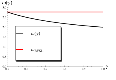
Fig. 21-a	Fig. 21-b

Figure 21: The contour of integration over $z$ in Eq. (A)(see Fig. 21-a) and the values of $\omega=-E_{a\to\infty}$ for the analytical estimates given by Eq. (A)(see Fig. 21-b). The red line shows the intercept of the BFKL Pomeron.

References

- [1] L. V. Gribov, E. M. Levin and M. G. Ryskin, Phys. Rep. 100 (1983) 1.
- [2] A. H. Mueller and J. Qiu, Nucl. Phys. B268 (1986) 427.
-
[3]
L. McLerran and R. Venugopalan,
Phys. Rev. D49 (1994) 2233, 3352; D50 (1994) 2225;
D53 (1996) 458;
D59 (1999) 094002. - [4] Yuri V Kovchegov and Eugene Levin, “ Quantum Choromodynamics at High Energies”, Cambridge Monographs on Particle Physics, Nuclear Physics and Cosmology, Cambridge University Press, 2012 and references therein.
- [5] A. Kovner and U. A. Wiedemann, Phys. Rev. D 66, 051502 (2002) [hep-ph/0112140].
- [6] A. Kovner and U. A. Wiedemann, Phys. Rev. D 66, 034031 (2002) [hep-ph/0204277].
- [7] A. Kovner and U. A. Wiedemann, Phys. Lett. B 551, 311 (2003) [hep-ph/0207335].
- [8] E. Ferreiro, E. Iancu, K. Itakura and L. McLerran, Nucl. Phys. A 710, 373 (2002) [hep-ph/0206241].
-
[9]
M. Froissart,
Phys. Rev. 123 (1961) 1053;
A. Martin, “Scattering Theory: Unitarity, Analitysity and Crossing.” Lecture Notes in Physics, Springer-Verlag, Berlin-Heidelberg-New-York, 1969. - [10] E. A. Kuraev, L. N. Lipatov, and F. S. Fadin, Sov. Phys. JETP 45, 199 (1977); Ya. Ya. Balitsky and L. N. Lipatov, Sov. J. Nucl. Phys. 28, 822 (1978).
- [11] L. N. Lipatov, Phys. Rep. 286 (1997) 131; Sov. Phys. JETP 63 (1986) 904 [Zh. Eksp. Teor. Fiz. 90, 1536 (1986)].
- [12] J. Berger and A. M. Stasto, Phys. Rev. D 84, 094022 (2011) [arXiv:1106.5740 [hep-ph]].
- [13] J. Berger and A. Stasto, Phys. Rev. D 83, 034015 (2011) [arXiv:1010.0671 [hep-ph]].
- [14] K. J. Golec-Biernat and A. M. Stasto, Nucl. Phys. B 668, 345 (2003) [hep-ph/0306279].
- [15] E. Gotsman, M. Kozlov, E. Levin, U. Maor and E. Naftali, Nucl. Phys. A 742, 55 (2004) [hep-ph/0401021].
- [16] E.Levin and S.Tapia, JHEP 1307, 183 (2013) arXiv:1304.8022 [hep-ph].
- [17] E. A. Kuraev, L. N. Lipatov, and F. S. Fadin, Sov. Phys. JETP 45, 199 (1977) [Zh. Eksp. Teor. Fiz. 72 (1977) 377]; Sov. Phys. JETP 44 (1976) 443 [Zh. Eksp. Teor. Fiz. 71 (1976) 840]; Phys. Lett. B 60 (1975) 50; L. N. Lipatov, Sov. J. Nucl. Phys. 23 (1976) 338 [Yad. Fiz. 23 (1976) 642].
- [18] J. Bartels, L. N. Lipatov and K. Peters, Nucl. Phys. B 772 (2007) 103 [hep-ph/0610303].
- [19] I. Gradstein and I. Ryzhik, Table of Integrals, Series, and Products, Fifth Edition, Academic Press, London, 1994.
- [20] R. Enberg, K. J. Golec-Biernat and S. Munier , Phys. Rev. D 72, 074021 (2005) [hep-ph/0505101].
- [21] V. N. Gribov, “Space-time description of hadron interactions at high-energies,” hep-ph/0006158; Sov. J. Nucl. Phys. 9 (1969) 369 [Yad. Fiz. 9 (1969) 640].
- [22] P.Hartman, “ Ordinary differential equations”, second ed., Birkhuser, Boston-Basel-Stuttgart, 1982; I. N. Sneddon, “ Elements of partial differential equations”, Mc-Graw-Hill, New York,1957.