Electronic nematic phase transition in the presence of anisotropy

Abstract

We study the phase diagram of electronic nematic instability in the presence of $xy$ anisotropy. While a second order transition cannot occur in this case, mean-field theory predicts that a first order transition occurs near van Hove filling and its phase boundary forms a wing structure, which we term a Griffiths wing, referring to his original work of He³-He⁴ mixtures. When crossing the wing, the anisotropy of the electronic system exhibits a discontinuous change, leading to a meta-nematic transition, i.e., the analog to a meta-magnetic transition in a magnetic system. The upper edge of the wing corresponds to a critical end line. It shows a non-monotonic temperature dependence as a function of the external anisotropy and vanishes at a quantum critical end point for a strong anisotropy. The mean-field phase diagram is, however, very sensitive to fluctuations of the nematic order parameter, yielding a topologically different phase diagram. The Griffiths wing is broken into two pieces. A tiny wing appears close to zero anisotropy and the other is realized for a strong anisotropy. Consequently three quantum critical end points are realized. We discuss that these results can be related to various materials including a cold atom system.

I introduction

Nematic liquid crystals are well known. Rodlike molecules flow like a liquid, but are always oriented to a certain direction in the nematic phase. This state is characterized by breaking of the orientational symmetry, retaining the other symmetries of the system. Electrons are point particles, not molecules. Nevertheless electronic analogs of the nematic liquid crystals were observed in a number of interacting electron systems: Two-dimensional electron gases M. P. Lilly, K. B. Cooper, J. P. Eisenstein, L. N. Pfeiffer, and K. W. West (1999); R. R. Du, D. C. Tsui, H. L. Stormer, L. N. Pfeiffer, K. W. Baldwin, K. W. West (1999), high-temperature superconductors of cuprates Kivelson et al. (2003); M. Vojta (2009) and pnictides I. R. Fisher, L. Degiorgi, and Z. X. Shen (2011), the bilayer strontium ruthenate Sr₃Ru₂O₇ A. P. Mackenzie, J. A. N. Bruin, R. A. Borzi, A. W. Rost, and S. A. Grigera (2012), and an actinide material URu₂Si₂ R. Okazaki, T. Shibauchi, H. J. Shi, Y. Haga, T. D. Matsuda, E. Yamamoto, Y. Onuki, H. Ikeda, and Y. Matsuda (2011).

The electronic nematic order couples directly to an external anisotropy, which is thus expected to play a crucial role in a system exhibiting nematicity. The external anisotropy can be controlled by applying a uniaxial pressure, (epitaxial) strain, and sometimes by a crystal structure due to orthorhombicity. While it is generally not easy to quantify how much anisotropy is imposed on a sample, the anisotropy was calibrated recently by exploiting the piezoelectric effect J.-H. Chu, H.-H. Kuo, J. G. Analytis, and I. R. Fisher (2012). A nematic susceptibility was then extracted and its divergence was demonstrated near a nematic critical point.

Motivated by the experimental progress to control the external anisotropy, we study a role of the external anisotropy for the electronic nematic instability. This fundamental issue has not been well addressed even in mean-field theory. In particular, we focus on the nematicity associated with a $d$-wave Pomeranchuk instability ($d$PI) yam (a); Halboth and Metzner (2000), which is expected to exhibit interesting physics. In a mean-field theory in the absence of anisotropy Khavkine et al. (2004); Yamase et al. (2005), the $d$PI occurs around van Hove filling with a dome-shaped transition line. The transition is of second order at high temperatures and changes to first order at low temperatures. The end points of the second order line are tricritical points.

The presence of a tricritical point (TCP) implies a wing structure when a conjugate field to the corresponding order parameter is applied to the system. This insight originates from the study of He³-He⁴ mixtures by Griffiths R. B. Griffiths (1970). However, the conjugate field to the superfluid order parameter is not accessible in experiments. The wing structure predicted by Griffiths, which we term the Griffiths wing, was not tested for He³-He⁴ mixtures.

It was found that itinerant ferromagnetism occurs generally via a first order transition at low temperatures and a second order one at high temperatures D. Belitz, T. R. Kirkpatrick, and J. Rollbühler (2005). The end point of the second order line is a TCP. The order parameter is magnetization and its conjugate field is a magnetic field in that case. Similar to Griffiths’s work R. B. Griffiths (1970), a wing structure emerges from the first order transition line and extends to the side of a finite magnetic field. When crossing the wing, the system exhibits a jump of the magnetization, leading to a metamagnetic transition. Recently, the Griffiths wings were clearly observed in ferromagnetic metals such as UGe₂ H. Kotegawa, V. Taufour, D. Aoki, G. Knebel, and J. Flouqet (2011) and UCoAl D. Aoki, T. Combier, V. Taufour, T. D. Matsuda, G. Knebel, H. Kotegawa, and J. Flouquet (2011).

In this paper, we study Griffiths wings of an electronic nematic phase transition associated with the $d$PI. A conjugate field to the nematic order parameter is $xy$ anisotropy, which is accessible in experiments. By applying the anisotropy, we obtain a wing structure. However, in contrast to previous studies R. B. Griffiths (1970); D. Belitz, T. R. Kirkpatrick, and J. Rollbühler (2005), the Griffiths wing exhibits a non-monotonic temperature dependence. Furthermore we find that the wing structure is very sensitive to fluctuations of the order parameter, leading to a phase diagram topologically different from the mean-field result. These results can be related to various materials including a cold atom system.

II model

We study electronic nematicity associated with the $d$PI in the presence of $xy$ anisotropy. Our minimal model reads

$$H=\sum_{{\bf k},\sigma}(\epsilon^{0}_{{\bf k}}-\mu)c^{\dagger}_{{\bf k}\sigma}c_{{\bf k}\sigma}-\frac{1}{2N}\sum_{{\bf q}}g({\bf q})n_{d}({\bf q})n_{d}(-{\bf q})-\mu_{d}n_{d}({\bf 0})\,,$$ (1)

where $c^{\dagger}_{{\bf k}\sigma}$ ($c_{{\bf k}\sigma}$) is the creation (annihilation) operator of electrons with momentum ${\bf k}$ and spin $\sigma$, $\mu$ is the chemical potential, and $N$ is the number of sites. The kinetic energy $\epsilon_{{\bf k}}^{0}$ is given by a usual tight binding dispersion on a square lattice,

$$\epsilon^{0}_{{\bf k}}=-2t(\cos k_{x}+\cos k_{y})-4t^{\prime}\cos k_{x}\cos k_{y}\,.$$ (2)

The interaction term describes a $d$-wave weighted density-density interaction Metzner et al. (2003); $n_{d}({\bf q})=\sum_{{\bf k},\sigma}d_{{\bf k}}c^{\dagger}_{{\bf k}-\frac{{\bf q}}{2}\sigma}c_{{\bf k}+\frac{{\bf q}}{2}\sigma}$ with a $d$-wave form factor such as $d_{{\bf k}}=\cos k_{x}-\cos k_{y}$. The coupling strength $g({\bf q})$ has a peak at ${\bf q}=0$, that is, forward scattering dominates. This interaction drives a $d$PI at low temperatures and is obtained in microscopic models such as the $t$-$J$ yam (a), Hubbard Halboth and Metzner (2000); Valenzuela and Vozmediano (2001), and general models with central forces J. Quintanilla, M. Haque, and A. J. Schofield (2008), and also from dipole-dipole interaction C. Lin, E. Zhao, and W. V. liu (2010). A new aspect of the present study lies in the third term in Eq. (1). This term is expressed as $-\mu_{d}\sum_{{\bf k},\sigma}(\cos k_{x}-\cos k_{y})c^{\dagger}_{{\bf k}\sigma}c_{{\bf k}\sigma}$, and imposes an anisotropy of the nearest neighbor hopping integral $t$ between the $x$ and $y$ direction as easily seen from Eqs. (1) and (2). A value of $\mu_{d}$ is controlled by applying a uniaxial pressure and a strain, and also by an orthorhombic crystal structure. $\mu_{d}$ may be interpreted as the $d$-wave chemical potential in the sense that it couples to the $d$-wave weighted charge density. Since the order parameter of the $d$PI is proportional to $n_{d}({\bf 0})$, $\mu_{d}$ is a conjugate field to that and plays an essential role to generate a Griffiths wing associated with the $d$PI.

The interaction term in Eq. (1) is generated by spin-exchange yam (a); Miyanaga and Yamase (2006); B. Edegger, V. N. Muthukumar, and C. Gros (2006); M. Bejas, A. Greco, and H. Yamase (2012), Coulomb interaction Halboth and Metzner (2000); Valenzuela and Vozmediano (2001); weg ; S. Okamoto, D. Sénéchal, M. Civelli, and A.-M. Tremblay (2010); S.-Q. Su and T. A. Maier (2011), central forces J. Quintanilla, M. Haque, and A. J. Schofield (2008), and dipole-dipole interaction N. Lin, E. Gull, and A. Millis (2010). Hence various models can exhibit a strong tendency toward the $d$PI at low-energy scale, especially when the Fermi surface is close to saddle points around $(\pi,0)$ and $(0,\pi)$ where the $d$-wave form factor is enhanced. Our Hamiltonian (1) is applicable to such a situation and is regarded as a low-energy effective model of the $d$PI, independent of microscopic details. There can occur a competition with other tendencies such as superconductivity and magnetism in microscopic models, but Hamiltonian (1) does not contain interactions other than the $d$PI. Thus a competing physics is beyond the scope of the present study. Instead we wish to clarify a role of anisotropy in a rather general setup, focusing on the nematic physics. Although the interaction term might gain an anisotropic term especially for a large value of $\mu_{d}$, we believe that the conceptional basis of the Griffiths wings associated with nematicity is captured by Hamiltonian (1).

Hamiltonian (1) with $\mu_{d}=0$, namely without anisotropy, was already studied in mean-field theory Khavkine et al. (2004); Yamase et al. (2005). It was found Yamase et al. (2005) that the mean-field phase diagram of the $d$PI is characterized by a single energy scale. As a result, there exist various universal ratios charactering the phase diagram, which nicely captures experimental observations in Sr₃Ru₂O₇ Yamase (2007); H. Yamase (2013). The presence of momentum transfer ${\bf q}$ in the second term in Eq. (1) allows fluctuations around the mean-field solution. In an isotropic case ($\mu_{d}=0$), it was shown that nematic order-parameter fluctuations change a first order transition obtained in a mean-field theory into a continuous one when the fluctuations become sufficiently strong P. Jakubczyk, W. Metzner, and H. Yamase (2009); further stronger fluctuations can even destroy completely the nematic instability H. Yamase, P. Jakubczyk, and W. Metzner (2011). Nematic fluctuations close to a nematic quantum critical point lead to non-Fermi liquid behavior Oganesyan et al. (2001); Metzner et al. (2003); Garst and Chubukov (2010). It was also found that thermal nematic fluctuations near a nematic phase transition lead to a pronounced broadening of the quasi-particle peak with a strong momentum dependence characterized by the form factor $d_{{\bf k}}^{2}$, leading to a Fermi-arc like feature Yamase and Metzner (2012). A role of $xy$ anisotropy $(\mu_{d}\neq 0)$ was studied in the context of competition of a nematic instability and $d$-wave pairing instability yam (a); S. Okamoto, D. Sénéchal, M. Civelli, and A.-M. Tremblay (2010); S.-Q. Su and T. A. Maier (2011). It was emphasized that a given anisotropy to the system can be strongly enhanced due to nematic correlations. This feature was discussed to explain the strong anisotropy of magnetic excitation spectra Hinkov et al. (2004); V. Hinkov, P. Bourges, S. Pailhès, Y. Sidis, A. Ivanov, C. D. Frost, T. G. Perring, C. T. Lin, D. P. Chen, and B. Keimer (2007); V. Hinkov, D. Haug, B. Fauqué, P. Bourges, Y. Sidis, A. Ivanov, C. Bernhard, C. T. Lin, and B. Keimer (2008); Yamase and Metzner (2006); Yamase (2009) and the Nernst coefficient R. Daou, J. Chang, D. LeBoeuf, O. Cyr-Choinière, F. Laliberté, N. Doiron-Leyraud, B. J. Ramshaw, R. Liang, D. A. Bonn, W. H. Hardy, and L. Taillefer (2010); Hackl and Vojta (2009) in high-temperature superconductors. Except for these studies, a role of $xy$ anisotropy in the nematic physics is poorly understood even in mean-field theory. This issue is addressed in terms of our Hamiltonian (1) including the effect of fluctuations on mean-field results.

We consider a phase diagram in the three-dimensional space spanned by $\mu$, $\mu_{d}$, and temperature $T$. The phase diagram is symmetric with respect to the axis of $\mu_{d}=0$ and is almost symmetric with respect to the axis of $\mu=0$ as long as $t^{\prime}$ is small. Hence we focus on the region of $\mu>0$ and $\mu_{d}>0$ by taking $t^{\prime}=0$. Considering previous studies in He³-He⁴ mixtures R. B. Griffiths (1970) and ferromagnetic systems D. Belitz, T. R. Kirkpatrick, and J. Rollbühler (2005), we may expect a wing structure emerging from a first order transition of the $d$PI by applying the field $\mu_{d}$. The upper edge of the wing is a critical end line (CEL), which is determined by the condition

$$\frac{\partial\omega}{\partial\phi}=\frac{\partial^{2}\omega}{\partial\phi^{2}}=\frac{\partial^{3}\omega}{\partial\phi^{3}}=0\,,$$ (3)

where $\omega$ is the Gibbs free energy per lattice sites and $\phi$ is the order parameter of the $d$PI. Below all quantities of dimension of energy are presented in units of $t$.

III Mean-field analysis

We first study Hamiltonian (1) in a mean-field theory. The interaction term is decoupled by introducing the order parameter

$$\phi=gn_{d}({\bf 0})\,,$$ (4)

where $g=g({\bf 0})>0$. The mean-field Hamiltonian then reads

$$H_{MF}=\sum_{{\bf k},\sigma}\xi_{{\bf k}}c_{{\bf k}\sigma}^{\dagger}c_{{\bf k}\sigma}+\frac{N}{2g}\phi^{2}\,,$$ (5)

with the renormalized band

$$\xi_{{\bf k}}=\epsilon_{{\bf k}}^{0}-\mu-(\phi+\mu_{d})d_{{\bf k}}\,.$$ (6)

Obviously the conjugate field $\mu_{d}$ breaks $xy$ symmetry and plays the same role as the order parameter $\phi$. It is straightforward to obtain the free energy

$$\omega(\phi)=-\frac{2T}{N}\sum_{{\bf k}}\log\left(1+{\rm e}^{-\xi_{{\bf k}}/T}\right)+\frac{1}{2g}\phi^{2}\,$$ (7)

and we solve Eq. (3) numerically.

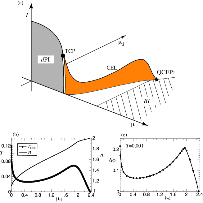
Figure 1: (Color online) Mean-field results. (a) Schematic phase diagram in the space spanned by $\mu$, $\mu_{d}$, and $T$. At $\mu_{d}=0$ a $d$PI occurs around van Hove filling, from which $\mu$ is measured. The transition is of second order at high $T$ (solid line) and of first order at low $T$ (double line). The solid circle denotes the TCP. The BI state is realized in the striped region. The wing (colored in orange) stands almost vertically on the plane of $\mu$ and $\mu_{d}$ close to van Hove filling and vanishes at the QCEP₁; the index 1 implies that the system is almost one dimensional. The upper edge of the wing (solid line) is a CEL. (b) Temperature of the CEL ($T_{\rm CEL}$) as a function of $\mu_{d}$; The wing is projected on the plane of $\mu_{d}$ and $T$. The electron density at $T_{\rm CEL}$ is also plotted. (c) Jump of the nematic order parameter across the wing at $T=0.001$.

Figure 1(a) is a schematic mean-field phase diagram mis (a). At zero anisotropy ($\mu_{d}=0$) a $d$PI occurs via a first order transition at low $T$ as already found in previous studies Khavkine et al. (2004); Yamase et al. (2005). With increasing $\mu$, the band is eventually filled up and the band insulating (BI) state is realized in the striped region. Its phase boundary is given by $\mu=4t$ for $\mu_{d}<2$ and $\mu=2\mu_{d}$ for $\mu_{d}>2$ mis (b). A wing emerges from the first order line and extends to a region of a finite $\mu_{d}$. The wing stands nearly vertically on the plane of $\mu_{d}$ and $\mu$ plane, and evolves close to van Hove filling on that plane. To see the wing structure more closely, we project the CEL on the plane of $\mu_{d}$ and $T$ in Fig. 1(b). The temperature of the CEL, $T_{\rm CEL}$, is rapidly suppressed by applying the anisotropy $\mu_{d}$, but does not go to zero. It recovers to form a broad peak around $\mu_{d}=2$ and eventually vanishes when it touches the BI phase, leading to a quantum critical end point (QCEP) there. In fact, the electron density becomes two at the QCEP as seen in Fig. 1(b). When the system crosses the wing, the nematic order parameter exhibits a jump, leading to a meta-nematic transition. Such a jump, $\Delta\phi$, is plotted in Fig. 1(c) along the bottom of the wing as a function of $\mu_{d}$. The magnitude of the jump exhibits behavior similar to $T_{\rm CEL}$. It is interesting that $\Delta\phi$ around $\mu_{d}=2$ becomes comparable to that at $\mu_{d}=0$ in spite of the presence of a large external anisotropy.

Figure 1 can be understood in terms of the $d$-wave weighted density of states, $N_{d}(\mu)=\frac{1}{N}\sum_{{\bf k}}d_{{\bf k}}^{2}\delta(\xi_{{\bf k}})$. This quantity appears in the second condition in Eq. (3), i.e., $\frac{\partial^{2}\omega}{\partial\phi^{2}}=0$, and diverges at van Hove filling unless the $d$-wave form factor vanishes at the saddle points. One can easily check that Eq. (3) is fulfilled close to such van Hove filling, leading to the Griffiths wing there. While the field $\mu_{d}$ modifies a band structure as $t_{x}=t(1+\mu_{d}/2t)$ and $t_{y}=t(1-\mu_{d}/2t)$, the saddle points of the non-interacting band dispersion remain at $(\pi,0)$ and $(0,\pi)$ as long as $\mu_{d}<2$. However, for $\mu_{d}>2$, the saddle pints shift to $(\pi,\pi)$ and $(0,0)$. Around $\mu_{d}=2$, therefore, the band becomes very flat, yielding a substantial enhancement of the density of states. This is the reason why $T_{\rm CEL}$ as well as $\Delta\phi$ exhibits a peak around $\mu_{d}=2$; the peak position is slightly deviated from $\mu_{d}=2$ because of the presence of a finite order parameter $\phi$. Since the saddle points $(\pi,\pi)$ and $(0,0)$ do not contribute to $N_{d}(\mu)$ because the $d$-wave form factor $d_{{\bf k}}$ vanishes there, $T_{\rm CEL}$ is suppressed for $\mu_{d}>2$ and ultimately vanishes near the band edge. Since $\mu_{d}$ is very large close to the QCEP₁, the system is almost one dimensional mis (c). Therefore we find a remarkable property that the Griffiths wing interpolates between a two- and (effectively) one-dimensional system by controlling the anisotropy.

IV effect of order-parameter fluctuations

In a mean-field theory we pick up the component with ${\bf q}={\bf 0}$ in Hamiltonian (1) [see also Eq. (4)]. Contributions from a finite ${\bf q}$ describe order-parameter fluctuations around the mean-field results. We address such fluctuation effects on the mean-field phase diagram. Since the Griffiths wing is realized near the van Hove singularity, a usual polynomial expansion of the order-parameter potential Hertz (1976) is not valid there. To circumvent such a problem, we employ a functional renormalization-group (fRG) scheme W. Metzner, M. Salmhofer, C. Honerkamp, V. Meden, and K. Schönhammer (2012). This scheme allows us to analyze fluctuations without any expansion of the potential Wetterich (1993) and was successfully applied to studies of fluctuation effects of the $d$PI in an isotropic case ($\mu_{d}=0$) P. Jakubczyk, W. Metzner, and H. Yamase (2009); H. Yamase, P. Jakubczyk, and W. Metzner (2011).

We use a path-integral formalism and follow a usual procedure to derive an order-parameter action Hertz (1976). We first decouple the fermionic interaction in Eq. (1) by introducing a Hubbard-Stratonovich field associated with the fluctuating order parameter of the $d$PI and then integrate fermionic degrees of freedom. Because we are interested in low-energy, long-wavelength fluctuations of the $d$PI, we retain the leading momentum and frequency dependencies of the two-point function and neglect such dependencies in high-order vertex functions. The resulting order-parameter action becomes

$$S[\phi]=\frac{1}{2}\sideset{}{{}^{\prime}}{\sum}_{q}\left[\phi_{q}\left(A_{0}\frac{|\omega_{n}|}{|{\bf q}|}+Z_{0}{\bf q}^{2}\right)\phi_{-q}\right]+{\cal U}[\phi]\,,$$ (8)

where $\phi_{q}$ with $q=({\bf q},\omega_{n})$ denotes the momentum representation of the order-parameter field $\phi$ and $\omega_{n}=2\pi nT$ with integer $n$ denotes the bosonic Matsubara frequencies. The approximation scheme of our action (8) corresponds to the next-leading order of derivative expansion. Hence the momenta and frequencies contributing to the action $S[\phi]$ should be restricted by the cutoff $\Lambda_{0}$ to the region $\frac{A_{0}|\omega_{n}|}{Z_{0}|{\bf q}|}+{\bf q}^{2}\leq\Lambda_{0}^{2}$, as emphasized by adding the prime in the summation in Eq. (8). In the fermionic representation, $\Lambda_{0}$ may be related to the maximal momentum transfer allowed by the interaction in the second term in Hamiltonian (1). If $\Lambda_{0}$ is set to be zero, the action (8) reproduces the mean-field theory. Physically, therefore, the value of $\Lambda_{0}$ controls the strength of order-parameter fluctuations. The effective potential ${\cal U}[\phi]$ is given by ${\cal U}[\phi]=\int_{0}^{\frac{1}{T}}d\tau\int d^{2}{\bf r}\,U[\phi({\bf r},\tau)]$, where $U(\phi)$ is equal to the mean-field potential [Eq. (7)] and we do not expand it in powers of $\phi$, in contrast to the usual case Hertz (1976).

We carry out calculations in the one-particle irreducible scheme of the fRG by computing the flow of the effective action $\Gamma^{\Lambda}[\phi]$ in the presence of an infrared cutoff $\Lambda$ W. Metzner, M. Salmhofer, C. Honerkamp, V. Meden, and K. Schönhammer (2012); $\Lambda$ is a quantity independent of $\Lambda_{0}$. In this scheme $\Gamma^{\Lambda}[\phi]$ interpolates between the bare action $S[\phi]$ [Eq. (8)] at the ultraviolet cutoff $\Lambda^{\rm UV}$ and the thermodynamic potential $\omega(\phi)$ in the limit of $\Lambda\to 0$. Its evolution is given by the functional exact flow equation Wetterich (1993),

$$\partial_{\Lambda}\Gamma^{\Lambda}\left[\phi\right]=\frac{1}{2}{\rm tr}\frac{\partial_{\Lambda}R^{\Lambda}}{\Gamma_{2}^{\Lambda}\left[\phi\right]+R^{\Lambda}}\,,$$ (9)

where $R^{\Lambda}$ is a regulator and $\Gamma_{2}^{\Lambda}\left[\phi\right]=\delta^{2}\Gamma^{\Lambda}[\phi]/\delta\phi^{2}$. We choose a Litim-type regulator D. F. Litim (2001) used in previous works P. Jakubczyk, W. Metzner, and H. Yamase (2009); H. Yamase, P. Jakubczyk, and W. Metzner (2011): $R^{\Lambda}=\left[Z\left(\Lambda^{2}-{\bf q}^{2}\right)-A\frac{|\omega_{n}|}{|{\bf q}|}\right]\theta\left(Z\left(\Lambda^{2}-{\bf q}^{2}\right)-A\frac{|\omega_{n}|}{|{\bf q}|}\right)$. A form of $\Gamma^{\Lambda}[\phi]$ is highly complicated and we parameterize it as

$$\Gamma^{\Lambda}[\phi]=\frac{1}{2}\sideset{}{{}^{\prime}}{\sum}_{q}\left[\phi_{q}\left(A^{\Lambda}\frac{|\omega_{n}|}{|{\bf q}|}+Z^{\Lambda}{\bf q}^{2}\right)\phi_{-q}\right]+{\cal U}^{\Lambda}[\phi]\,,$$ (10)

the same functional form as Eq. (8). We allow flows of $Z^{\Lambda}$ and ${\cal U}^{\Lambda}$, but discard the flow of $A^{\Lambda}$, which is of minor importance P. Jakubczyk, P. Strack, A. A. Katanin, and W. Metzner (2008) and is assumed to be $A^{\Lambda}=A_{0}$. Inserting Eq. (10) into Eq. (9) and evaluating the resulting equations for uniform fields, we obtain the flow equations of $Z^{\Lambda}$ and $U^{\Lambda}$; their derivations contain technical details and thus are left to the Appendix. By solving these flow equations numerically by reducing $\Lambda$ from $\Lambda^{\rm UV}$ to zero, we can determine the thermodynamic potential $\omega(\phi)$, which carries over the effect of nematic order-parameter fluctuations. To determine the Griffiths wing, we then search for a solution of Eq. (3) in the three-dimensional space spanned by $\mu$, $\mu_{d}$, and $T$. All these computations are performed numerically and require highly accurate numerics, otherwise higher order derivatives of the free energy, which are contained in Eq. (3), would not become smooth enough to conclude a phase diagram.

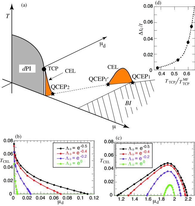
Figure 2: (Color online) Results in the presence of weak nematic order-parameter fluctuations. (a) Schematic phase diagram. The $d$PI phase is slightly suppressed by fluctuations. The wing obtained in Fig. 1(a) is broken into two pieces: one tiny wing close to $\mu_{d}=0$ and the other wing for a large $\mu_{d}$. The indices of QCEP₂ and QCEP${}_{1^{\prime}}$ imply that the system can be regarded to be two and quasi-one dimensional, respectively, at the QCEP. The dashed line corresponds to a crossover. The BI phase is assumed to be the same as the mean-field result. (b) and (c) The wings are projected on the plane of $\mu_{d}$ and $T$ for several choices of the cutoff $\Lambda_{0}$. (d) The critical anisotropy of the hopping integral to obtain the QCEP₂ as a function of the ratio of the tricritical temperature and its mean-field value.

Figure 2(a) is a schematic phase diagram in the presence of order-parameter fluctuations. The $d$PI phase diagram at zero anisotropy is slightly suppressed by fluctuations, but retains essentially the same features as the mean-field result. Applying the anisotropy $\mu_{d}$, the CEL is rapidly suppressed, leading to a tiny wing terminating at a QCEP₂. We then have a crossover region depicted by the dashed line. The order parameter of the $d$PI shows a rapid change, but without a jump, by crossing the dashed line. With further increasing $\mu_{d}$, another wing emerges with two QCEPs. While the Griffiths wing might seem to be broken up into two separate pieces by fluctuations, the two wings are actually connected via a crossover line [dashed line in Fig. 2(a)] as reminiscence of a single Griffiths wing in the absence of fluctuations

These results may be understood as originating from a unique feature of the mean-field result, namely the suppression of $T_{\rm CEL}$ in an intermediate region of $\mu_{d}$ in Fig. 1(b). Given that $\phi$ enters the renormalized dispersion Eq. (6), it is easily expected that fluctuations of $\phi$ blur the van Hove singularity and yield the suppression of the density of states. Consequently, relatively low $T_{\rm CEL}$ obtained in the mean-field theory is easily suppressed to become zero, leading to the breaking of the Griffiths wing.

In Figs. 2(b) and (c) two Griffiths wings are projected on the plane of $\mu_{d}$ and $T$. The results are shown for several choices of the cutoff $\Lambda_{0}$, which controls the strength of fluctuations; a larger $\Lambda_{0}$ means stronger fluctuations. When $\Lambda_{0}$ becomes larger, the CELs are suppressed more as expected. This suppression is, however, quite remarkable. To quantify the suppression, we consider the critical external anisotropy, $\Delta t_{c}/t=\frac{t_{x}-t_{y}}{t_{x}+t_{y}}=\mu_{d}/2t$, to obtain a QCEP. We plot $\Delta t_{c}/t$ in Fig. 2(d) as a function of the ratio of the tricritical temperature and its mean-field value ($T_{\rm TCP}/T_{\rm TCP}^{\rm MF}$) as the strength of fluctuations. We see that when $T_{\rm TCP}$ is suppressed by fluctuations, for example, by half, a very small anisotropy ($\Delta t_{c}/t\approx 0.01)$ is sufficient to yield a QCEP. Furthermore the strength of fluctuations to realize the QCEP is weak in the sense that the $d$PI phase diagram at $\mu_{d}=0$ is still well captured by mean-field theory. Therefore we conclude that the Griffiths wing is very sensitive to fluctuations and the QCEP₂ can be reached with a weak anisotropy even though the transition is of first order at zero anisotropy. This is sharply different from the mean-field result [Fig. 1(a)] where a QCEP can be reached with a very strong anisotropy, i.e., $\Delta t_{c}/t\approx 1.2$ for $T_{\rm TCP}/T_{\rm TCP}^{\rm MF}=1$.

V Discussions

As mentioned in Sec. II, our Hamiltonian (1) is a low-energy effective model of an electronic nematic phase transition in the presence of $xy$ anisotropy. It addresses a situation where a nematic tendency becomes dominant at low energy, independent of microscopic details. Usually mean-field theory is powerful to discuss actual materials at least about qualitative features. However, the Griffiths wing turns out to be sensitive even to weak fluctuations, leading to the phase diagram (Fig. 2) qualitatively different from the mean-field phase diagram (Fig. 1). Since we may always have at least weak fluctuations of the order parameter in actual materials, Fig. 2 is expected to be more realistic than Fig. 1. Hence we bear Fig. 2 in mind and discuss relevance to various systems as well as theoretical implications for future studies.

Cuprates. Neutron scattering experiments showed that the magnetic excitation spectrum becomes anisotropic in momentum space. The anisotropy observed in YBa₂Cu₃O_6.85 and YBa₂Cu₃O_6.6 Hinkov et al. (2004); V. Hinkov, P. Bourges, S. Pailhès, Y. Sidis, A. Ivanov, C. D. Frost, T. G. Perring, C. T. Lin, D. P. Chen, and B. Keimer (2007) is relatively weak and is well captured in terms of competition of the tendency toward the $d$PI and pairing correlations Yamase and Metzner (2006). For YBa₂Cu₃O_6.45, however, Ref. V. Hinkov, D. Haug, B. Fauqué, P. Bourges, Y. Sidis, A. Ivanov, C. Bernhard, C. T. Lin, and B. Keimer, 2008 reported a very strong anisotropy, which could not be interpreted in the same theory as Ref. Yamase and Metzner, 2006. Instead two different theories were proposed: one invoking the presence of a nematic quantum critical point E.-A. Kim, M. J. Lawler, P. Oreto, S. Sachdev, E. Fradkin, and S. A. Kivelson (2008) and the other invoking a dominant nematic tendency over the pairing tendency Yamase (2009). The point is that the observed anisotropy seems to suddenly change by crossing the oxygen concentration around $6.45$.

Microscopic models of cuprates such as $t$-$J$ and Hubbard exhibit the $d$PI tendency as shown by various approximation schemes: slave-boson mean-field theory yam (a), exact diagonalization Miyanaga and Yamase (2006), variational Monte Carlo B. Edegger, V. N. Muthukumar, and C. Gros (2006), dynamical mean-field theory S. Okamoto, D. Sénéchal, M. Civelli, and A.-M. Tremblay (2010), dynamical cluster approximation S.-Q. Su and T. A. Maier (2011), and a large-$N$ expansion M. Bejas, A. Greco, and H. Yamase (2012). Furthermore our low-energy effective interaction [the second term in Eq. (1)] can be obtained from those microscopic models yam (a); Halboth and Metzner (2000); Valenzuela and Vozmediano (2001). The $t$-$J$ model yam (a); B. Edegger, V. N. Muthukumar, and C. Gros (2006); M. Bejas, A. Greco, and H. Yamase (2012) actually exhibits a nematic tendency very similar to the present mean-field result [Fig. 1 for $\mu_{d}=0$]. The nematicity in the $t$-$J$ model is strongly enhanced by approaching half-filling, which corresponds to van Hove filling of the spinon dispersion in the slave-boson mean-field theory P. A. Lee, N. Nagaosa, and X.-G. Wen (2006). While a competition with other tendencies is beyond the scope of the present theory, our low-energy theory is expected to capture the essential feature at least associated with the nematicity.

Superconducting samples of Y-based cuprates have an intrinsic $xy$ anisotropy coming from the CuO chain structure and its anisotropy is estimated around $\mu_{d}=0.03$-$0.04$ Yamase and Metzner (2006). Hence Y-based cuprates are located along the axis of a small $\mu_{d}$ in Fig. 2(a). With decreasing $\mu$ (hole picture), namely decreasing the oxygen concentration, the system can cross the tiny wing or pass close to the QCEP₂, which may explain a sudden change of the anisotropy observed in the magnetic excitation spectrum V. Hinkov, D. Haug, B. Fauqué, P. Bourges, Y. Sidis, A. Ivanov, C. Bernhard, C. T. Lin, and B. Keimer (2008). In this context, it is interesting to explore a possibility that the presence of a nematic quantum critical point assumed in previous studies E.-A. Kim, M. J. Lawler, P. Oreto, S. Sachdev, E. Fradkin, and S. A. Kivelson (2008); Y. Huh and S. Sachdev (2008) can be associated with the QCEP₂.

Ruthenates. The strontium ruthenate Sr₃Ru₂O₇ exhibits an electronic nematic instability around a magnetic field 8 T A. P. Mackenzie, J. A. N. Bruin, R. A. Borzi, A. W. Rost, and S. A. Grigera (2012). The system is tetragonal, namely $\mu_{d}=0$. The band structure calculations show six Fermi surfaces at zero magnetic field Hase and Nishihara (1997); Singh and Mazin (2001). There is a two-dimensional Fermi surface very close to the momenta $(\pi,0)$ and $(0,\pi)$, which contribute to the large density of states near the Fermi energy. Hence focusing on such a two-dimensional band near van Hove filling, the nematic instability in Sr₃Ru₂O₇ is frequently discussed in terms of a one-band model. The interaction term in Hamiltonian (1) is employed in various theoretical studies for Sr₃Ru₂O₇ Kee and Kim (2005); Doh et al. (2007); C. Puetter, H. Doh, and H.-Y. Kee (2007); yam (b); Ho and Schofield (2008); M. H. Fischer, and M. Sigrist (2010), which indeed capture major aspects of the experimental phase diagram except for a slope of the first order transition Yamase and Katanin (2007); Yamase (2007). Although the Zeeman field is not considered in the present theory, it simply splits the Fermi surfaces of the spin-up and spin-down band and then tunes the Fermi surface of either spin closer to van Hove filling, a very similar role to the chemical potential. In fact, explicit calculations including the Zeeman field confirm this consideration Kee and Kim (2005); Yamase and Katanin (2007); Yamase (2007); H. Yamase (2013). Therefore, on the basis of the present study (Fig. 2), we predict an emergence of a tiny Griffiths wing close to $\mu_{d}=0$ by applying a strain along the $x$ or $y$ direction in Sr₃Ru₂O₇ mis (d). If the system gains an anisotropy of in-plane lattice constants by $x$%, the anisotropy of $t$ is expected around $3.5x$% when hybridization between the Ru $d$ and O $p$ states is a major contribution to $t$ Harrison (1989). Since a required anisotropy of $t$ to reach a QCEP can become very small [see Fig. 2(d)], not only the rapid drop of the CEL, but also the QCEP can be observed in experiments.

Quasi-one-dimensional metals. A piece of the broken Griffiths wings is also realized for a strong anisotropy in Figs. 2(a) and (c). Such a strong anisotropy is intrinsically realized in quasi-one-dimensional metals. In this case, when the system is located close to van Hove filling, our theory predicts that the anisotropy of the electronic system can change dramatically by controlling a uniaxial pressure or carrier density. Although we are not aware of experiments discussing such a phenomenon, there are theoretical works reporting it in a different context qui and their meta-nematic transition can be interpreted as originating from a Griffiths wing. While $xy$ anisotropy of physical quantities in an already strongly anisotropic system was not likely recognized as something related to nematicity, we have revealed that the Griffiths wing interpolates between a two- and one-dimensional system. Moreover, various microscopic interactions can generate an attractive interaction of the $d$PI yam (a); Halboth and Metzner (2000); Valenzuela and Vozmediano (2001); J. Quintanilla, M. Haque, and A. J. Schofield (2008); N. Lin, E. Gull, and A. Millis (2010). Therefore we may reasonably wait for further experiments.

Cold atom systems. Each condensed matter system is characterized by a certain value of $\mu_{d}$, which is determined by an intrinsic property of the material such as a crystal structure and cannot be changed much externally. However, $\mu_{d}$ is fully tunable for optical lattices in a cold atom system I. Bloch, J. Dalibard, and W. Zwerger (2008); qui by changing the strength of laser beams between the $x$ and $y$ direction. One may employ cold fermions with a large dipolar moment and align the dipole along the $z$ direction. Dipolar interaction then yields a repulsive interaction between fermions, which leads to an attractive interaction of the $d$PI, i.e., the second term in Eq. (1) Valenzuela and Vozmediano (2001); C. Lin, E. Zhao, and W. V. liu (2010). The Griffiths wings are then expected near van Hove filling at temperatures well below the Fermi energy [Fig. 2(a)]. Such low temperatures are now accessible in experiments K. Aikawa, A. Frisch, M. Mark, S. Baier, R. Grimm, and F. Ferlaino (2014).

Anomalous ground state. Our obtained results (Fig. 2) contain interesting insights into electronic nematicity and will likely promote further theoretical studies. A non-Fermi liquid ground state is stabilized at a quantum critical point of the $d$PI Oganesyan et al. (2001); Metzner et al. (2003); Garst and Chubukov (2010). It is plausible to expect an anomalous ground state also at a QCEP of the $d$PI. In an intermediate region between the QCEP₂ and QCEP${}_{1^{\prime}}$, the dashed line in Fig. 2(a), quantum fluctuations completely wash out the wing even close to van Hove filling. If the system remains a Fermi liquid there, the density of states would diverge at van Hove filling. We would then expect a Griffiths wing there because our Hamiltonian (1) has an attractive interaction of the $d$PI. However, we have obtained a crossover around the dashed line in Fig. 2(a). This consideration hints a possible non-Fermi liquid ground state at van Hove filling; the same conclusion was obtained also by Dzyaloshinskii in a different context Dzyaloshinskii (1996). Therefore $xy$ anisotropy can lead to an anomalous ground state in a wide parameter space spanned by $\mu$ and $\mu_{d}$, even though the quantum phase transition is a first order at zero anisotropy. This possibility is very interesting because usually a non-Fermi liquid can be stabilized only at a certain point at zero temperature such as a quantum critical point, except for purely one-dimensional systems.

VI conclusions

Electronic nematic order couples directly to $xy$ anisotropy. The anisotropy can be controlled by applying a uniaxial pressure and a strain. Moreover, actual materials often contain intrinsic anisotropy due to a crystal structure such as orthorhombicity. The present theory addresses such a situation in a rather general setup by including the $d$-wave chemical potential $\mu_{d}$ in a low-energy effective Hamiltonian of an electronic nematic instability [see Eq. (1)]. Although the nematic physics is frequently discussed in a two-dimensional system, the present theory shows that the nematic physics is important also in an anisotropic system. We have shown that the Griffiths wing associateds with the nematicity interpolates between two- and (nearly) one-dimensional systems by changing the anisotropy (Figs. 1 and 2). In fact, a recent theoretical work qui reports a meta-nematic phenomena in an anisotropic system, which can be interpreted as coming from the Griffiths wing. The Griffiths wing of the nematicity is found to be quite unique in the sense that it exhibits a non-monotonic temperature dependence (Fig. 1), in sharp contrast to the cases of He³-He⁴ mixtures R. B. Griffiths (1970) and ferromagnetic systems D. Belitz, T. R. Kirkpatrick, and J. Rollbühler (2005); H. Kotegawa, V. Taufour, D. Aoki, G. Knebel, and J. Flouqet (2011); D. Aoki, T. Combier, V. Taufour, T. D. Matsuda, G. Knebel, H. Kotegawa, and J. Flouquet (2011). The Griffiths wing turns out to be very sensitive to nematic order-parameter fluctuations, leading to a phase diagram (Fig. 2) topologically different from the mean-field phase diagram: a QCEP close to zero anisotropy, a crossover region, and a broken Griffiths wing terminated with two QCEPs in a strong anisotropy. This suggests that even if fluctuations are relatively weak and the phase diagram is still well captured by mean-field theory at zero anisotropy, fluctuation effects can be dramatic once $xy$ anisotropy is introduced. Hence the effect of fluctuations is definitely important to the Griffiths wing. Given that order-parameter fluctuations are present to a greater or lesser extent in actual materials, our Fig. 2 is expected to be more realistic than Fig. 1. Not only at three QCEPs, but also in the crossover region, the ground state may feature non-Fermi liquid behavior. This possibility is very interesting since a non-Fermi liquid state can extend in a wide parameter space at zero temperature. We hope that the present theory serves as a fundamental basis of the nematic physics in various materials such as high-$T_{c}$ cuprates, double-layered ruthenates, quasi-one-dimensional metals, and cold atoms, and will promote further theoretical studies.

Appendix A

In this Appendix we present technical details of our fRG framework.

Our formalism of the fRG partly overlaps with previous works P. Jakubczyk, W. Metzner, and H. Yamase (2009); H. Yamase, P. Jakubczyk, and W. Metzner (2011), which studied how nematic fluctuations change the mean-field phase diagram for $\mu_{d}=0$. Compared with previous calculations P. Jakubczyk, W. Metzner, and H. Yamase (2009); H. Yamase, P. Jakubczyk, and W. Metzner (2011), we did the following extension. i) Introduction of two cutoffs, one is the physical cutoff $\Lambda_{0}$ which gives the upper cutoff to the summation in Eq. (8) as emphasized by adding the prime to the symbol $\Sigma$, and the other is the ultraviolet cutoff $\Lambda^{\rm UV}$ which is in principle infinite. In the previous formalism P. Jakubczyk, W. Metzner, and H. Yamase (2009); H. Yamase, P. Jakubczyk, and W. Metzner (2011) $\Lambda^{UV}$ was assumed to be identical to $\Lambda_{0}$. ii) No additional approximations to compute the right hand side of flow equations, that is, we take account of quantum fluctuations in the anomalous dimension $\eta=-\frac{{\partial}\log Z}{{\partial}\log\Lambda}$, the contribution from the term $\frac{\partial Z}{\partial\Lambda}$, and an additional term coming from the momentum derivative of the regular for the flow of $Z$.

The resulting flow equations become different from those in Refs. P. Jakubczyk, W. Metzner, and H. Yamase, 2009 and H. Yamase, P. Jakubczyk, and W. Metzner, 2011:

$$\Lambda\partial_{\Lambda}U(\phi)=\frac{T}{4\pi}\frac{1}{1+\frac{U^{\prime\prime}}{Z\Lambda^{2}}}\left\{\frac{2-\eta}{2}\left[\hat{\Lambda}^{2}+2\sum_{n=1}^{n_{\rm max}}(\hat{q}_{2}^{2}-\hat{q}_{1}^{2})\right]+\frac{\eta}{4\Lambda^{2}}\left[\hat{\Lambda}^{4}+2\sum_{n=1}^{n_{\rm max}}(\hat{q}_{2}^{4}-\hat{q}_{1}^{4})\right]\right\},$$ (11)

$$\Lambda\partial_{\Lambda}Z=-\eta Z,$$ (12)

and

$$\eta=\left\{\begin{array}[]{l}\frac{\displaystyle\frac{T}{4\pi}\frac{(U^{\prime\prime\prime})^{2}}{Z^{3}\Lambda^{6}(1+\frac{U^{\prime\prime}}{Z\Lambda^{2}})^{4}}\left[{\Lambda}^{2}+3\displaystyle\sum_{n=1}^{n_{\rm max}}(\hat{q}_{2}^{2}-\hat{q}_{1}^{2})\right]}{\displaystyle 1+\frac{T}{8\pi}\frac{(U^{\prime\prime\prime})^{2}}{Z^{3}\Lambda^{6}(1+\frac{U^{\prime\prime}}{Z\Lambda^{2}})^{4}}\displaystyle\sum_{n=1}^{n_{\rm max}}(\hat{q}_{2}^{2}-\hat{q}_{1}^{2})\left[4-\frac{3}{\Lambda^{2}}(\hat{q}_{2}^{2}+\hat{q}_{1}^{2})\right]}\quad{\rm for}\,\Lambda\leq\Lambda_{0},\\ 0\quad{\rm for}\,\Lambda>\Lambda_{0}.\end{array}\right.$$ (13)

$U^{\prime\prime}(U^{\prime\prime\prime})$ denotes the second (third) derivative with respect to $\phi$; $n_{\rm max}$ is the maximum Matsubara frequency contributing to the flow equations and is given by $n_{\rm max}=\left[\frac{Z\hat{\Lambda}^{3}}{3\pi\sqrt{3}A_{0}T}\right]$; $\hat{q}_{1}(>0)$ and $\hat{q}_{2}(\geq\hat{q}_{1})$ are real roots of the equation

$$q^{3}-\hat{\Lambda}^{2}q+\frac{A_{0}}{Z}|\omega_{n}|=0\,;$$ (14)

and

$$\hat{\Lambda}=\left\{\begin{array}[]{l}\Lambda\quad{\rm for}\quad\Lambda\leq\Lambda_{0},\\ \Lambda_{0}\quad{\rm for}\quad\Lambda>\Lambda_{0}.\end{array}\right.$$ (15)

We solve the differential equations (11) and (12) numerically by reducing $\Lambda$ from $\Lambda^{\rm UV}$ to zero; the initial condition is given by the bare action Eq. (8). Since we cannot set $\Lambda^{\rm UV}=\infty$ numerically, we first did calculations for various choices of large $\Lambda^{\rm UV}$ and checked that our conclusions do not depend on the value of $\Lambda^{\rm UV}(\geq\Lambda_{0})$. In addition, our conclusions also do not depend on a precise choice of $A_{0}$ and $Z_{0}$. We took $\Lambda^{\rm UV}=\Lambda_{0}$, $A_{0}=1$, and $Z_{0}=10$ in Fig. 2.

References

- M. P. Lilly, K. B. Cooper, J. P. Eisenstein, L. N. Pfeiffer, and K. W. West (1999) M. P. Lilly, K. B. Cooper, J. P. Eisenstein, L. N. Pfeiffer, and K. W. West, Phys. Rev. Lett. 82, 394 (1999).
- R. R. Du, D. C. Tsui, H. L. Stormer, L. N. Pfeiffer, K. W. Baldwin, K. W. West (1999) R. R. Du, D. C. Tsui, H. L. Stormer, L. N. Pfeiffer, K. W. Baldwin, K. W. West, Solid State Commun. 109, 389 (1999).
- Kivelson et al. (2003) S. A. Kivelson, I. P. Bindloss, E. Fradkin, V. Oganesyan, J. M. Tranquada, A. Kapitulnik, and C. Howald, Rev. Mod. Phys. 75, 1201 (2003).
- M. Vojta (2009) M. Vojta, Adv. Phys. 58, 699 (2009).
- I. R. Fisher, L. Degiorgi, and Z. X. Shen (2011) I. R. Fisher, L. Degiorgi, and Z. X. Shen, Rep. Prog. Phys. 74, 124506 (2011).
- A. P. Mackenzie, J. A. N. Bruin, R. A. Borzi, A. W. Rost, and S. A. Grigera (2012) A. P. Mackenzie, J. A. N. Bruin, R. A. Borzi, A. W. Rost, and S. A. Grigera, Physica C 481, 207 (2012).
- R. Okazaki, T. Shibauchi, H. J. Shi, Y. Haga, T. D. Matsuda, E. Yamamoto, Y. Onuki, H. Ikeda, and Y. Matsuda (2011) R. Okazaki, T. Shibauchi, H. J. Shi, Y. Haga, T. D. Matsuda, E. Yamamoto, Y. Onuki, H. Ikeda, and Y. Matsuda, Science 331, 439 (2011).
- J.-H. Chu, H.-H. Kuo, J. G. Analytis, and I. R. Fisher (2012) J.-H. Chu, H.-H. Kuo, J. G. Analytis, and I. R. Fisher, Science 337, 710 (2012).
- yam (a) H. Yamase and H. Kohno, J. Phys. Soc. Jpn. 69, 332 (2000); 69, 2151 (2000).
- Halboth and Metzner (2000) C. J. Halboth and W. Metzner, Phys. Rev. Lett. 85, 5162 (2000).
- Khavkine et al. (2004) I. Khavkine, C.-H. Chung, V. Oganesyan, and H.-Y. Kee, Phys. Rev. B 70, 155110 (2004).
- Yamase et al. (2005) H. Yamase, V. Oganesyan, and W. Metzner, Phys. Rev. B 72, 035114 (2005).
- R. B. Griffiths (1970) R. B. Griffiths, Phys. Rev. Lett. 24, 715 (1970).
- D. Belitz, T. R. Kirkpatrick, and J. Rollbühler (2005) D. Belitz, T. R. Kirkpatrick, and J. Rollbühler, Phys. Rev. Lett. 94, 247205 (2005).
- H. Kotegawa, V. Taufour, D. Aoki, G. Knebel, and J. Flouqet (2011) H. Kotegawa, V. Taufour, D. Aoki, G. Knebel, and J. Flouqet, J. Phys. Soc. Jpn. 80, 083703 (2011).
- D. Aoki, T. Combier, V. Taufour, T. D. Matsuda, G. Knebel, H. Kotegawa, and J. Flouquet (2011) D. Aoki, T. Combier, V. Taufour, T. D. Matsuda, G. Knebel, H. Kotegawa, and J. Flouquet, J. Phys. Soc. Jpn. 80, 094711 (2011).
- Metzner et al. (2003) W. Metzner, D. Rohe, and S. Andergassen, Phys. Rev. Lett. 91, 066402 (2003).
- Valenzuela and Vozmediano (2001) B. Valenzuela and M. A. H. Vozmediano, Phys. Rev. B 63, 153103 (2001).
- J. Quintanilla, M. Haque, and A. J. Schofield (2008) J. Quintanilla, M. Haque, and A. J. Schofield, Phys. Rev. B 78, 035131 (2008).
- C. Lin, E. Zhao, and W. V. liu (2010) C. Lin, E. Zhao, and W. V. liu, Phys. Rev. B 81, 045115 (2010).
- Miyanaga and Yamase (2006) A. Miyanaga and H. Yamase, Phys. Rev. B 73, 174513 (2006).
- B. Edegger, V. N. Muthukumar, and C. Gros (2006) B. Edegger, V. N. Muthukumar, and C. Gros, Phys. Rev. B 74, 165109 (2006).
- M. Bejas, A. Greco, and H. Yamase (2012) M. Bejas, A. Greco, and H. Yamase, Phys. Rev. B 86, 224509 (2012).
- (24) I. Grote, E. Körding, and F. Wegner, J. Low Temp. Phys. 126, 1385 (2002); V. Hankevych, I. Grote, and F. Wegner, Phys. Rev. B 66, 094516 (2002).
- S. Okamoto, D. Sénéchal, M. Civelli, and A.-M. Tremblay (2010) S. Okamoto, D. Sénéchal, M. Civelli, and A.-M. Tremblay, Phys. Rev. B 82, 180511 (2010).
- S.-Q. Su and T. A. Maier (2011) S.-Q. Su and T. A. Maier, Phys. Rev. B 84, 220506(R) (2011).
- N. Lin, E. Gull, and A. Millis (2010) N. Lin, E. Gull, and A. Millis, Phys. Rev. B 82, 045104 (2010).
- Yamase (2007) H. Yamase, Phys. Rev. B 76, 155117 (2007).
- H. Yamase (2013) H. Yamase, Phys. Rev. B 87, 195117 (2013).
- P. Jakubczyk, W. Metzner, and H. Yamase (2009) P. Jakubczyk, W. Metzner, and H. Yamase, Phys. Rev. Lett. 103, 220602 (2009).
- H. Yamase, P. Jakubczyk, and W. Metzner (2011) H. Yamase, P. Jakubczyk, and W. Metzner, Phys. Rev. B 83, 125121 (2011).
- Oganesyan et al. (2001) V. Oganesyan, S. A. Kivelson, and E. Fradkin, Phys. Rev. B 64, 195109 (2001).
- Garst and Chubukov (2010) M. Garst and A. V. Chubukov, Phys. Rev. B 81, 235105 (2010).
- Yamase and Metzner (2012) H. Yamase and W. Metzner, Phys. Rev. Lett. 108, 186405 (2012).
- Hinkov et al. (2004) V. Hinkov, S. Pailhès, P. Bourges, Y. Sidis, A. Ivanov, A. Kulakov, C. T. Lin, D. Chen, C. Bernhard, and B. Keimer, Nature (London) 430, 650 (2004).
- V. Hinkov, P. Bourges, S. Pailhès, Y. Sidis, A. Ivanov, C. D. Frost, T. G. Perring, C. T. Lin, D. P. Chen, and B. Keimer (2007) V. Hinkov, P. Bourges, S. Pailhès, Y. Sidis, A. Ivanov, C. D. Frost, T. G. Perring, C. T. Lin, D. P. Chen, and B. Keimer, Nat. Phys. 3, 780 (2007).
- V. Hinkov, D. Haug, B. Fauqué, P. Bourges, Y. Sidis, A. Ivanov, C. Bernhard, C. T. Lin, and B. Keimer (2008) V. Hinkov, D. Haug, B. Fauqué, P. Bourges, Y. Sidis, A. Ivanov, C. Bernhard, C. T. Lin, and B. Keimer, Science 319, 597 (2008).
- Yamase and Metzner (2006) H. Yamase and W. Metzner, Phys. Rev. B 73, 214517 (2006).
- Yamase (2009) H. Yamase, Phys. Rev. B 79, 052501 (2009).
- R. Daou, J. Chang, D. LeBoeuf, O. Cyr-Choinière, F. Laliberté, N. Doiron-Leyraud, B. J. Ramshaw, R. Liang, D. A. Bonn, W. H. Hardy, and L. Taillefer (2010) R. Daou, J. Chang, D. LeBoeuf, O. Cyr-Choinière, F. Laliberté, N. Doiron-Leyraud, B. J. Ramshaw, R. Liang, D. A. Bonn, W. H. Hardy, and L. Taillefer, Nature (London) 463, 519 (2010).
- Hackl and Vojta (2009) A. Hackl and M. Vojta, Phys. Rev. B 80, 220514(R) (2009).
- mis (a) Figure 1(a) does not depend on the value of and we took in Figs. 1(b) and (c).
- mis (b) In the presence of a small (), the BI is realized for for and for .
- mis (c) If is included, the system always allows a hopping along the diagonal direction. Hence the anisotropy of does not necessary mean that the system becomes fully one dimensional.
- Hertz (1976) J. A. Hertz, Phys. Rev. B 14, 1165 (1976).
- W. Metzner, M. Salmhofer, C. Honerkamp, V. Meden, and K. Schönhammer (2012) W. Metzner, M. Salmhofer, C. Honerkamp, V. Meden, and K. Schönhammer, Rev. Mod. Phys. 84, 299 (2012).
- Wetterich (1993) C. Wetterich, Phys. Lett. B 301, 90 (1993).
- D. F. Litim (2001) D. F. Litim, Phys. Rev. D 64, 105007 (2001).
- P. Jakubczyk, P. Strack, A. A. Katanin, and W. Metzner (2008) P. Jakubczyk, P. Strack, A. A. Katanin, and W. Metzner, Phys. Rev. B 77, 195120 (2008).
- E.-A. Kim, M. J. Lawler, P. Oreto, S. Sachdev, E. Fradkin, and S. A. Kivelson (2008) E.-A. Kim, M. J. Lawler, P. Oreto, S. Sachdev, E. Fradkin, and S. A. Kivelson, Phys. Rev. B 77, 184514 (2008).
- P. A. Lee, N. Nagaosa, and X.-G. Wen (2006) P. A. Lee, N. Nagaosa, and X.-G. Wen, Rev. Mod. Phys. 78, 17 (2006).
- Y. Huh and S. Sachdev (2008) Y. Huh and S. Sachdev, Phys. Rev. B 78, 064512 (2008).
- Hase and Nishihara (1997) I. Hase and Y. Nishihara, J. Phys. Soc. Jpn. 66, 3517 (1997).
- Singh and Mazin (2001) D. J. Singh and I. I. Mazin, Phys. Rev. B 63, 165101 (2001).
- Kee and Kim (2005) H.-Y. Kee and Y. B. Kim, Phys. Rev. B 71, 184402 (2005).
- Doh et al. (2007) H. Doh, Y. B. Kim, and K. H. Ahn, Phys. Rev. Lett. 98, 126407 (2007).
- C. Puetter, H. Doh, and H.-Y. Kee (2007) C. Puetter, H. Doh, and H.-Y. Kee, Phys. Rev. B 76, 235112 (2007).
- yam (b) H. Yamase, Phys. Rev. Lett. 102, 116404 (2009); Phys. Rev. B 80, 115102 (2009).
- Ho and Schofield (2008) A. F. Ho and A. J. Schofield, Europhys. Lett. 84, 27007 (2008).
- M. H. Fischer, and M. Sigrist (2010) M. H. Fischer, and M. Sigrist, Phys. Rev. B 81, 064435 (2010).
- Yamase and Katanin (2007) H. Yamase and A. A. Katanin, J. Phys. Soc. Jpn. 76, 073706 (2007).
- mis (d) While an anisotropy is also generated by introducing a magnetic field along the or direction A. P. Mackenzie, J. A. N. Bruin, R. A. Borzi, A. W. Rost, and S. A. Grigera (2012), the coupling to electrons is different from our anisotropic field of .
- Harrison (1989) W. A. Harrison, Electronic structure and the properties of solids (Dover, 1989).
- (64) J. Quintanilla, S. T. Carr, and J. J. Betouras, Phys. Rev. A 79, 031601(R) (2009); S. T. Carr, J. Quintanilla, and J. J. Betouras, Phys. Rev. B 82, 045110 (2010).
- I. Bloch, J. Dalibard, and W. Zwerger (2008) I. Bloch, J. Dalibard, and W. Zwerger, Rev. Mod. Phys. 80, 885 (2008).
- K. Aikawa, A. Frisch, M. Mark, S. Baier, R. Grimm, and F. Ferlaino (2014) K. Aikawa, A. Frisch, M. Mark, S. Baier, R. Grimm, and F. Ferlaino, Phys. Rev. Lett. 112, 010404 (2014).
- Dzyaloshinskii (1996) I. Dzyaloshinskii, J. Phys. I France 6, 119 (1996).