The Formation and Evolution of Small Star Clusters

Abstract

Recent observations show that small, young, stellar groupings of $\sim 10$ to 40 members tend of have a centrally-located most massive member, reminiscent of mass segregation seen in large clustered systems. Here, we analyze hydrodynamic simulations which form small clusters and analyze their properties in a manner identical to the observations. We find that the simulated clusters possess similar properties to the observed clusters, including a tendency to exhibit mass segregation. In the simulations, the central location of the most massive member is not due to dynamical evolution, since there is little interaction between the cluster members. Instead, the most massive cluster member appears to form at the center. We also find that the more massive stars in the cluster form at slightly earlier times.

1 Introduction

Stars typically do not form in isolation but rather within groups of a hundred or more stars (Lada & Lada, 2003). Even star-forming regions that have low-stellar densities, e.g., Taurus, contain clear groups of 10 or more stars (Kirk & Myers 2011, hereafter KM11). The pervasiveness of stellar clustering from the very earliest embedded phase of star formation (e.g., Gutermuth et al 2009, hereafter G09) to old, dense globular clusters (e.g., Meylan & Heggie 1997) indicates that the nature of stellar distributions holds clues about the formation and dynamical evolution of stars.

In local star-forming regions, Bressert et al. (2010) find that the distribution of protostellar separations has no characteristic scale. One interpretation of this result is that there is no obvious preferred scale to separate “clustered” stars from “non-clustered” stars. Simulations suggest that clustering can be dynamically erased rapidly or may, when present, provide no distinctive signature in the separation distribution (Gieles et al., 2012; Parker & Meyer, 2012). However, singling out higher density concentrations is nonetheless instructive because the most densely distributed stars are most likely to gravitationally interact and evolve as an ensemble.

A variety of definitions exist to dictate what is a stellar cluster. Lada & Lada (2003) propose a minimum of 35 “physically related” stars with total mass density $>1.0{\rm M}_{\mathord{\odot}}$ pc^-3. This definition is derived by requiring that a grouping survive evaporation for 10⁸ years. To be applied in practice, the Lada & Lada (2003) cluster definition and other similar approaches (e.g., Jørgensen et al., 2008) use stellar surface density thresholds to determine cluster membership. A number of authors have recently utilized a different method, the minimal spanning tree (MST), to define stellar groups (Cartwright & Whitworth, 2004; Gutermuth et al., 2009; Allison et al., 2009; Maschberger et al., 2010; Maschberger & Clarke, 2011; Kirk & Myers, 2011; Parker & Meyer, 2012). An MST is essentially a structure which connects all points together through their minimum distances, much like the sketch of a constellation. We adopt the MST method for identifying stellar groups for easier comparison with observational results. Ultimately, all methods work to identify regions of relatively high stellar density but are subject to some subjective decision about the location of the cluster boundary.

Inspection of the highest stellar density regions indicates that the most massive stars tend to be located closer to cluster centers and in the highest stellar density regions (Hillenbrand & Hartmann, 1998a; Gouliermis et al., 2004). This appears to be true also for clusters where the most massive star is only a few solar masses (KM11). Since it is only possible to assign stellar mass after an age of a couple million years, at which point most of the natal cloud gas has been accreted or expelled, it is difficult to determine the primordial distribution of masses.

Numerical simulations thus provide an important avenue for exploring early cluster properties. Early work modeled the dynamical evolution of small clusters by beginning with a set of stellar seeds in a gas potential (Bonnell et al., 1997, 2001; Delgado-Donate et al., 2003). In later work, simulations also followed the formation of individual stars from the gravitational collapse of dense gas cores (e.g., Klessen 2001; Bate et al. 2003; Bonnell et al. 2004; Offner et al. 2008; Girichidis et al. 2011). However, even with the aid of simulations it remains unclear whether observed mass segregation is primordial or dynamical and depends partially on the assumed model and initial conditions (e.g., Bonnell & Davies, 1998). For example, N-body simulations of clumpy, subvirial (i.e., collapsing) clusters find that mass segregation can occur within a global dynamical time of the full system (Allison et al., 2009; Parker et al., 2013). In contrast, Maschberger et al. (2010) find that marginally bound hydrodynamic simulations produce mass segregation within 0.5 Myr of formation. Girichidis et al. (2012) find that the steepness of the initial large-scale gas density profile from which stars are formed also affects the final spatial distribution of stellar masses.

In principle, the details of clustering and mass segregation can be used to differentiate between theoretical models. In practice, however, it is uncertain whether observed early mass segregation favors the turbulent core model (Krumholz et al., 2007) or competitive accretion model (Bonnell et al., 2001). In the former scenario, massive stars form from high-column density gas, which is incidentally often centrally located. In the latter scenario, stars forming at the cloud center are deep within the gravitational well and thus have the largest reservoir of available gas, which allows them to grow to higher masses.

Most simulation analyses have focussed on systems representing larger-cluster formation, including the formation of massive stars and high stellar density environments. We focus here on the less-explored regime of the formation of small ($N$=10-40), sparse (1-10’s $pc^{-2}$) intermediate mass ($M<4$ M_⊙) stellar groups comparable to those in KM11. In this regime, stellar dynamics might be expected to play a smaller role, although KM11 do observe mass segregation at an early age. We also investigate the effect of global cloud properties, such as Mach number, temperature, and turbulent driving scale, on cluster properties.

Our work extends previous studies in several important ways. First, we quantitatively define subclusters within the simulation and then follow the evolution of these groups and their properties over several cluster dynamical times for a range of cloud properties. Second, we apply observational constraints and quantitatively compare the simulated cluster properties with observations of similar clusters. Finally, we analyze simulations with continuous turbulent energy injection rather than simulations of isolated clouds wherein turbulence is allowed to decay. The former picture is more similar to the “distributed” star formation in nearly regions, which have relatively low stellar surface densities and are not strongly centrally condensed.

In Section 2 we describe our simulation parameter study. In Section 3 we discuss the identification of stellar groups using minimal spanning trees (MST). We analyze the cluster properties in Section 4, including the details of the mass distributions and member separations. In Section 5 we compare with observations of young clusters. Finally, we summarize our conclusions in Section 6.

2 Numerical Simulations

We analyze six simulations of molecular clouds forming stars. We perform all simulations with the ORION adaptive mesh refinement (AMR) code (Truelove et al., 1998; Klein, 1999). The simulations do not include magnetic fields and five assume a simple isothermal equation of state. The simulation procedure is described in Offner et al. (2009) and Offner et al. (2013), so we give only a brief summary here.

We initialize the simulations with uniform density and then perturb the gas for two to three crossing times using a random velocity field. This field has a flat power spectrum over wavenumbers $k_{1}$ to $k_{2}$ (see Table 1), and we renormalize the perturbations to maintain a constant cloud velocity dispersion. After the initial driving phase that produces a well-mixed turbulent distribution, we turn on gravity and allow collapse to proceed.

The simulations each have a 256³ base grid and four levels of AMR refinement, where we automatically add new grids to satisfy the Jeans criterion and adopt a Jeans number of 0.125 (Truelove et al., 1997). We introduce a sink particle when the Jeans condition is violated on the finest level (Krumholz et al., 2004). These particles approximately represent young stellar objects, and henceforth, we shall refer to them as “stars.” Since we do not include mass loss due to protostellar outflows, the simulated particle masses should be considered upper limits. We also merge particles if they approach within four fine cells and if one has $m_{*}\leq 0.1~{}{\rm M}_{\mathord{\odot}}$. The sink particle-gas interaction is smoothed on scales of one fine cell, such that the dynamics of closely approaching particles, especially when their mass is comparable to the cell gas mass, is not well modeled. In any event, we expect the formation of small fragments to be suppressed with the addition of either radiative transfer or magnetic fields (e.g, Offner et al., 2009; Commerçon et al., 2011). Thus, our stars may also sometimes represent binary or multiple star systems rather than individual stars.

Table 1 displays the simulation parameters. The parameters of the fiducial Rm6 simulation are set such that the cloud is virialized:

$$\alpha=\frac{5\sigma^{2}(L/2)}{GM}=1,$$ (1)

where $L$ is the cloud size, $M$ is the cloud mass, and $\sigma=\mathcal{M}c_{s}/\sqrt{3}$ is the one-dimensional velocity dispersion, where $c_{s}$ is the sound speed. The fiducial simulation also obeys the observed linewidth-size relation (e.g., Solomon et al., 1987; McKee & Ostriker, 2007):

$$\sigma=0.72\left(\frac{R}{1{\rm pc}}\right)^{0.5}{\rm km~{}s}^{-1}.$$ (2)

The other simulations vary in temperature, Mach number, driving scale, and physics. Table 1 illustrates that the differences lead to significant statistical differences in the number density of stars. For reference, simulation Rm6s has parameters identical to Rm6 but uses a different turbulent random seed and produces a similar surface density of stars, $n_{*}$, to the Rm6 simulation.

Table 1: Simulation Properties

Runa	$L$a	$M$a	Ta	$\mathcal{M}$ a	$k_{1}..k_{2}$a	$n_{*}$b	t${}_{end}^{c}$	$N_{*}^{c}$	$SFE^{c}$
	(pc)	(${\rm M}_{\mathord{\odot}}$)	(K)			(pc-2)	(Myr)		(%)
Rm6d	2	600	10	6.6	1..2	18.2	0.95	88	17.6
Rm6s	2	600	10	6.6	1..2	18.8	0.95	100	18.1
Rm9d	2	600	10	8.9	1..2	3.2	0.95	17	3.5
Rm4d	2	600	10	4.2	1..2	13.8	0.89	80	10.4
Rk34	2	600	10	6.6	3..4	3.2	0.91	14	2.6
Rt20	2	600	20	6.6	1..2	1.5	0.95	17	3.8
Rrte	0.65	185	10	6	1..2	30.6	0.32	18	7.2

^aSimulation ID, box length, total initial gas mass, initial gas temperature, and Mach number, respectively.

^bThe projected number density of stars after one freefall time including only those stars with $m_{*}>0.03~{}{\rm M}_{\mathord{\odot}}$.

^cThe time elapsed in the simulation after gravity was turned on, and the total number of stars, and star formation efficiency (stellar mass divided by total mass) at this final time.

^dProperties of this simulation were previously analysed in Offner et al. (2013).

^eThis simulation from Offner et al. (2009) includes radiative transfer; it models heating due to accretion and nuclear burning.

3 Cluster Identification

3.1 Simulated Stellar Catalogs

Our method of cluster identification was designed to mimic that in KM11. The location of stars formed within the simulations was first projected onto three planes ($xy$, $xz$, and $yz$), as an observer would view the simulated region from a large distance away along the $z$, $y$, and $x$ axes. Since the simulations are performed within a periodic box, we replicate the simulated stellar distribution to a total of three by three boxes, to ensure any clusters with members across a box edge are properly identified. In our final analysis, only clusters identified which have centres within the inner box are included, to ignore duplicate clusters.

In real molecular clouds, dense, star-forming cores are estimated to lose about two-thirds of their mass to protostellar outflows and winds before the final mass of the star is set, assuming that there is a one-to-one mapping between the dense core and initial stellar mass function (e.g., Alves et al., 2007). Since outflows are not included in these simulations, we reduce the masses of the sink particles formed by two thirds; the exact factor used has little effect on our final results, the majority of which involve relative stellar masses. We eliminate any sink particles which have re-scaled masses of $<0.03$ M_⊙. Observationally, YSOs at very low masses become difficult to detect; the surveys analyzed by KM11 suffer from incompleteness around 0.01 to 0.03 M_⊙. Finally, in each of the three projected views, we remove the lower mass member of any pairs separated by less than 1000 AU. This separation corresponds to the approximate resolution limit of the stellar catalogs analyzed by KM11. Since the observed stellar masses were derived from spectral types, any low-mass companions closer than the minimum resolution would not have been counted in the observational mass estimate. Note that our results are not strongly sensitive to the precise choice in cutoff values; the main effect is to slightly change the value of L_crit used to define clusters (discussed in the following section). In Appendix A, we demonstrate that our final results are robust to changes in L_crit. We note that the simulations without radiative feedback likely over-estimate the amount of fragmentation on small scales (Offner et al., 2009; Bate, 2009). By excluding very small stars and the smaller member of close pairs, which we do in order to adhere to observational limits, we also correct for this effect.

3.2 MST Identification

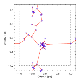
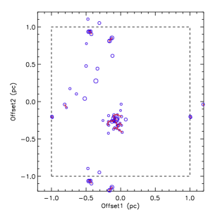
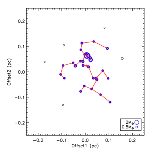
With this final set of simulated stellar catalogs, we identify small stellar clusters for each of the three projections using minimum spanning trees. An MST represents the minimum total length by which all points can be connected (e.g. Barrow et al., 1985); each connecting line segment is referred to as a branch. Once the full MST structure is calculated, we follow the procedure of G09 and KM11 to identify clusters. Figure 1 shows an example of this full procedure.

Figure 1: The minimal spanning tree structure computed for the Rm6 simulation at the final time step (0.95 Myr) when viewed along the $z$ axis ($xy$ projection). The original simulation is contained within the dashed square, while the outer borders show part of the replicated boxes. The blue circles show the locations of the sink particles, with their size scaling with mass (see legend in right panel), while the red lines show the MST structure. Note that additional clustered structure occurs across the original simulation boundaries. Left: The full MST structure. Middle: The MST structure remaining after branches with lengths larger than $L_{crit}$ (here 0.07 pc) have been removed. Groupings of more than ten sink particles which remain connected are classified as clusters. Right: A close-up view of the single cluster found in this example. Here, non-members are shown in black, and the cluster centre is indicated by the red plus sign.

In the left panel of Figure 1, the full MST structure is shown for the $xy$ projection of the Rm6 simulation at its final time step (0.95 Myr). Since the simulation has been replicated three times in either direction to allow us to account for the effect of periodic boundaries, several structures can be seen more than once. For clarity, only a small portion of the outer replicated simulation boxes are displayed.

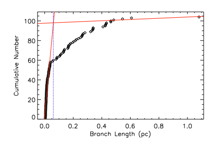
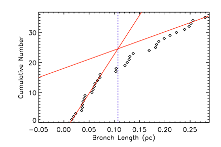
Within the full MST structure, clusters are visually apparent as regions of small star-star separations, i.e., stars connected by short branches. Clusters can therefore be defined as stars all interconnected by branch lengths less than some value, the critical branch length, L_crit. G09 found that nearby clustered regions have MSTs with a characteristic cumulative distribution of branch lengths: a steep rise at small branch lengths followed by a turn-over to a shallow slope, illustrated in Figure 10. Given this characteristic cumulative branch length distribution, the branch length of the turn-over is an obvious choice for L_crit, and that is effectively what G09 and KM11 adopt. Appendix A discusses the determination of L_crit in more detail. With such a procedure, regions which have different mean clustering properties have different L_crit values, which more naturally captures the local stellar overdensities than adopting a constant value would do. In KM11, there is a factor of a few difference between L_crit found for the sparse stellar distribution in Taurus compared with the much denser clustered IC 348.

For our analysis of the simulations, if we followed an identical method, we would potentially have a different L_crit measured for each simulation, at each time step, in each of the three viewing angles. With the analysis in Appendix A, we demonstrate that it is sufficient for our purposes to adopt a single constant value of L_crit for each simulation (i.e., no variation with time or viewing angle). We do not find strong evidence for real variations in L_crit within each simulation, and maintaining a single L_crit allows for easier intercomparisons within each simulation. Allowing for a different L_crit between the various simulations is important, as different initial conditions can result in different clustering properties. The L_crit adopted for each simulation is given in Table 2.

Table 2: MST statistics

Sim	Lcrit a	Medianb	Meanb	Minb	Maxb	Lratc
	(pc)	(pc)	(pc)	(pc)	(pc)
Rk34	0.12	0.21	0.34	0.007	1.2	0.027
Rm4	0.06	0.05	0.13	0.004	1.1	0.013
Rm6	0.07	0.04	0.10	0.005	0.95	0.016
Rm6s	0.07	0.05	0.09	0.005	0.6	0.013
Rm9	0.1d	0.40	0.37	0.005	0.75	0.022
Rrt	0.1d	0.12	0.12	0.016	0.3	0.061
Rt20	0.1	0.14	0.25	0.005	1.2	0.025

^aThe critical branch length used for identifying clusters in the simulation (all projections, all time steps).
^bThe median, mean, minimum, and maximum branch lengths in the final time step of each simulation, averaged over all three projections.
^cThe ratio of $L_{crit}$ to the maximum projected separation between sources in the final time step of each simulation, averaged over all three projections.
^d$L_{crit}$ is poorly determined due to the small number of sources.

As can be seen in Table 2, L_crit varies by a factor of about two between the different simulations, ranging from 0.06 pc to 0.12 pc. In KM11, the relatively sparse Taurus stars have an L_crit of 0.52 pc, while the tightly clustered stars in IC348 have an L_crit of 0.083 pc; G09 found L_crit values between 0.086 pc and 0.7 pc in their sample. The values of L_crit measured in the simulations span a smaller range than these two observational surveys, and tend to be small. The L_crit values are, however, larger than that used in Maschberger et al. (2010) (of 0.025 pc) for the analysis of a competitive accretion simulations showing the formation of a larger, more densely clustered region. The MST analysis in Girichidis et al. (2012) is restricted to the $\Lambda_{MST}$ method of Allison et al. (2009), which, in the case of large-$N$ clusters without substructure, can be an effective method to measure mass segregation. The $\Lambda_{MST}$ method does not require L_crit to be determined, however, a small L_crit would be expected, given the high stellar densities in the simulations.

A second statistic associated with L_crit is the ratio of L_crit to the maximum separation between stars. In observed clusters, regions with sparser clusters such as Taurus tend to have a larger L_crit values as well as a larger maximum separation between stars. In denser clusters, both L_crit and the maximum separation between stars are smaller, and L_crit (and by definition, also the maximum separation) has also been found to increase when a more extended, sparser, region around a cluster is included in the analysis (Masiunas et al., 2012). We find that the ratio of L_crit to the maximum separation between stars is relatively constant in the observations, ranging from 1% to 3% for the clusters in KM11. Performing a comparable measurement on the simulations reveals that they are generally consistent with the observations, as shown in Table 2. All of the simulations except for Rrt have ratios between 1% and 3%, while in Rrt, the ratio is 6%. Rrt was one of two simulations where the value of L_crit measured was highly uncertain, so the poorer agreement with observations is perhaps unsurprising.

Once L_crit is determined, and the initial full MST structure is “pruned” of all branches longer than L_crit(middle panel of Figure 1); stars which remain connected through short branches are potential clusters. KM11 impose an additional criterion that clusters have more than ten members to allow for meaningful analysis of cluster properties. The right panel of Figure 1 shows a zoomed-in view of the cluster identified in the middle panel with the red plus showing the cluster’s centre. As in KM11, we define the centre as the median position of all cluster members; this is less prone to bias than, e.g., the mass-weighted mean position for measurements of mass segregation. In Appendix B we demonstrate that using instead the mean cluster member position as the cluster’s centre has little impact on our results.

4 Results

4.1 Mass Distribution

Figure 2: The distribution of stellar masses at the final time step of each simulation. The two runs of Rm6 with differing initial turbulent seeds are plotted in the same panel, with Rm6s shown by the dashed blue line. The dotted red line in each figures shows the the Kroupa IMF distribution (as given in Weidner et al., 2010), scaled to the same total number of stars, and given the same minimum mass cutoff. The numbers in the top right corner show the probability that the mass distribution in the simulation is drawn from the same parent sample as the Kroupa IMF.

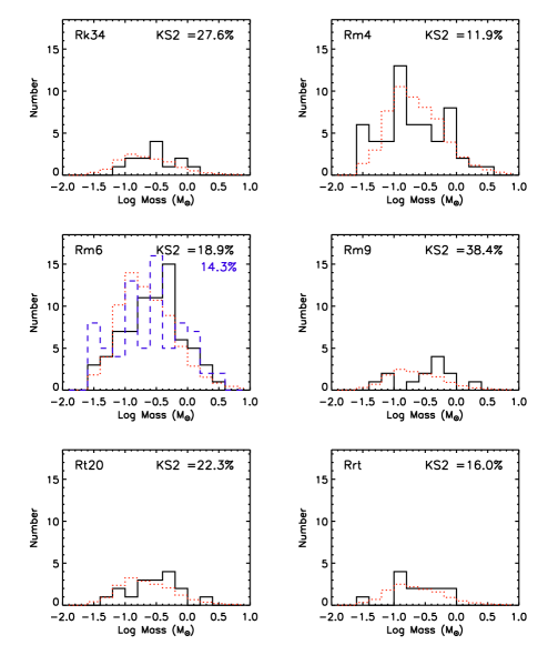
Figure 2 shows the stellar masses at the final time step in each simulation, with the masses reduced by a factor of 3 from the sink cell masses, and the observational limit of 0.03 M_⊙ applied. Earlier time steps generally follow the same trend but with fewer sources. Observed young stellar mass functions tend to be consistent with the standard IMF, with the possible exception of Taurus, which has a relative excess of sub-solar, K7-M1 type stars (e.g., Luhman et al., 2009). Figure 2 shows the stellar mass distributions (solid black lines) compared to the Kroupa IMF (red dotted line). The simulation mass distributions are consistent with a Kroupa IMF; a two-sided Kolmogorov-Smirnov test (e.g., Conover, 1999) gives probabilities between 10 and 40% that the two are drawn from the same parent sample. We note that earlier time steps in the simulations give a similar result, and the two runs of Rm6 are statistically similar. For reference, the Jeans mass of Rm6 is $M_{J}=8.0{\rm M}_{\mathord{\odot}}$, where $M_{J}=4/3\pi\bar{\rho}(L_{J}/2.0)^{3}$ and the Jeans length is defined as $L_{J}=c_{s}[\pi/(G\bar{\rho})]^{1/2}$. This is slightly higher than the mean stellar mass we find in the simulations.

4.2 Mass Evolution

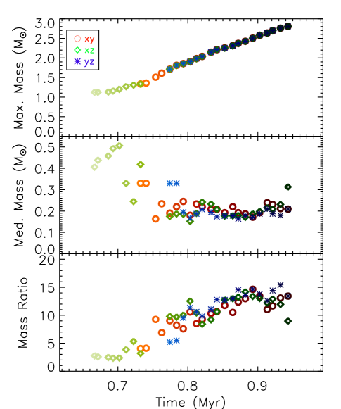
We next examine the stellar mass properties within each cluster identified. Figure 3 shows the evolution of the mass of the most massive cluster member for the Rm6 simulation, for each of the three projections, every 0.01 Myr (top panel). Note that only one cluster with more than 10 members was identified in each projection. The most massive star formed in this simulation is located within a bona-fide 3D clustering of sources, and hence the same point is plotted for the clusters identified in all three projected views. At early times, the cluster has fewer members, and due to the small motions of the stars near the cluster’s periphery, the grouping tends to alternate between meeting and not meeting the cluster definition (more than 10 members all connected by MST branch lengths of less than L_crit). This leads to some apparent gaps in the time-sampling plotted.

Figure 3 shows that the most massive cluster member tends to grow with time due to accretion, in this case, following a roughly linear trend. Accretion also occurs in the other stars in the simulation, however, this is less apparent when examining the median cluster member mass as a function of time (middle panel of Figure 3). At earlier times in particular, this accretion signature is masked by the addition of new cluster members. The majority of new cluster members are new stars which formed in the simulation (or stars which have now accreted sufficient material to surpass the observational threshold), and their addition to the cluster tends to decrease the median cluster mass. This effect is largest at the earlier times when the total number of cluster members is small. Other simulations have also been shown to produce time-independent IMFs that agree with the observed IMF (Krumholz et al., 2012; Bate, 2012). This is generally attributed to either stellar feedback or dynamical interactions regulating stellar masses. Since the IMF is observed to be robust to variation across a broad range of initial conditions and environments (Bastian et al., 2010), it is unlikely to have a preferred characteristic timescale.

The ratio of the mass of the most massive and median cluster members (the “mass ratio” shown in the bottom panel of Figure 3) gives a rough sense of how gravitationally dominant the most massive cluster member is expected to be in terms of the cluster’s dynamical evolution. We find that the mass ratio tends to increase slowly with time, spanning a slightly smaller range of values than the mass ratios found in KM11. This is discussed in more detail in Section 5.

Figure 3: The variation in maximum mass, median mass, and mass ratio in the Rm6 simulation as a function of time. Red circles, green diamonds, and blue asterisks show the results for the three projections, and earlier times are shown with lighter colours. The simulations were sampled every 0.01 Myr to provide more readable plots.

4.3 Separation Distribution

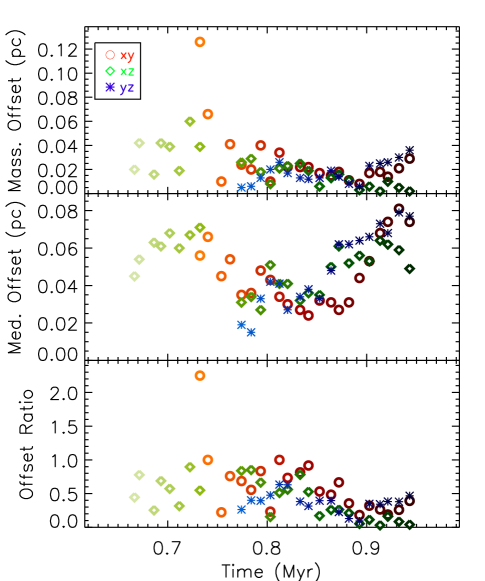
We similarly analyze the evolution of the spatial positions of the cluster members. The top panel of Figure 4 shows the evolution of the separation of the most massive cluster member in the Rm6 simulation from their cluster centres. From this figure, it is clear that the separation neither monotonically increases nor decreases – rather, it is variable. Much of this variability, and all instances of large changes between adjacent time steps, are caused by variations in cluster membership, rather than substantial motion of the most massive cluster member. Particularly at earlier times, when the total number of cluster members is small, the addition or subtraction of a cluster member on the outskirts (with a separation of roughly L_crit to its nearest neighbour), can cause a significant change in the cluster centre position. On rare occasions, a star near the cluster boundary may itself be separated from one or two additional non-cluster members by less than L_crit, in which case, when it becomes less than L_crit from an existing cluster member, either through motion or the appearance of a new star inbetween, the cluster gains several new members, and the cluster centre is more strongly influenced. The reverse situation can also occur – one or several cluster members near the outskirts which are separated by nearly L_crit from the next cluster members may move slightly farther away, reducing the overall cluster membership and changing the cluster centre accordingly. The motion of the most massive cluster member itself, contributes relatively little to the changes observed in Figure 4, and we discuss this in more detail in the following section.

The middle panel of Figure 4 shows the variation in the median value of all cluster member’s offsets from the centre with time. This variation is primarily due to the change in the cluster centre, induced by cluster membership changes. As with the most massive member’s offset, the large, sudden variation tend to be when multiple stars became members (non-members) due to small motions taking them below (above) the L_crit separation from the next nearest cluster member. Several of the large-scale variations in the median offset can also be seen in the massive star offset.

The bottom panel of Figure 4 shows the ratio of the most massive member’s offset to the median offset, the ‘offset ratio’, as a function of time. This ratio gives an indication of how centrally-located the most massive cluster member is: ratios much less than one imply that the most massive cluster member lies near the cluster centre, while ratios much larger than one would imply the opposite; randomly located most massive members tend to have offset ratios around one (KM11). The offset ratio shown in Figure 4 shows significant scatter, although slightly less than either the most massive star’s or median stars’ offsets individually, since both can be affected by changes to the location of the cluster centre in a similar manner. It is notable that the offset ratio tends to be less than one at all times in the simulation, for all projections, and there is no obvious evolution with time. These points will be discussed in more detail in Section 5.

Figure 4: The variation in offset from the cluster centre for the most massive member, the median cluster value, and the ratio of the two (the ‘offset ratio’) in the Rm6 simulation as a function of time, sampled every 0.01 Myr. Red circles, green diamonds, and blue asterisks show the clusters identified in each of the three projections, and lighter shades indicate earlier time steps.

4.4 Dynamical Evolution of Cluster Members

The previous results show significant mass segregation from the earliest times clusters are identified. A cluster by our definition, however, must have a minimum of eleven members, so it is possible that some dynamical evolution occurs prior to the times analyzed above. To assess the amount of dynamical evolution, in this section we investigate the motion of the most massive cluster members beginning from their time of formation. If the most massive member moves significantly and interacts dynamically with other stars, then the mass segregation displayed by the MST clusters may not in fact be primordial.

There are two timescales that are relevant to the process of dynamical mass segregation. An estimate for the mass segregation timescale is given by the time it takes the most massive member to migrate to the cluster center. For a star of mass $M$ in a cluster with $N$ stars this can be expressed:

$$t_{\rm seg}(m)\simeq\frac{{\langle M\rangle}}{M}t_{\rm relax}\simeq\frac{{\langle M\rangle}}{M}\frac{N}{8{~{}\rm ln}(N)}\frac{R}{{\langle v\rangle}},$$ (3)

where ${\langle v\rangle}$ is the average velocity of a star and $R$ is the cluster radius. (Spitzer, 1969; Allison et al., 2009). For stars initially moving with ${\langle v\rangle}\simeq c_{s}$, $N=15$, ${\langle M\rangle}=0.6{\rm M}_{\mathord{\odot}}$ and $R=0.2$ pc, a star of $3~{}{\rm M}_{\mathord{\odot}}$ will migrate to the cluster center in $t_{\rm seg}\sim 0.14$ Myr.

This estimate implicitly assumes that the system is gas free and that the gravitational potential is dominated by the stars. However, the simulated systems here are gas dominated, which acts to damp the effect of two-body interactions. Overall, less than 20% of the total gas in the simulations turns into stars by 1 $t_{\rm ff}$, although the volume restricted to the cluster itself likely has a higher mass fraction in stars. In a gas dominated system, the characteristic dynamical timescale can be approximated by the freefall time:

$$t_{\rm ff}=\left(\frac{3\pi}{32G\rho}\right)^{1/2},$$ (4)

where $\rho=\mu_{p}n$ is the mass density and $\mu_{p}=2.33m_{\rm H}$ is the mean particle mass. For a mean clump number density of $n=10^{4}$ cm^-3, $t_{\rm ff}=0.34$ Myr, which is slightly longer than the N-body dynamical times. Protostars form from the dense gas ($n>10^{5}$ cm^-3), which has a small relative offset velocity from the lower density core envelope gas (e.g., Kirk et al. 2007; Offner et al. 2009; Kirk et al. 2010), so a single star shouldn’t have a significantly different velocity than the gas it forms from. The core itself, however, may have some advection velocity, $t_{\rm adv}$, that is comparable to the sound speed or slightly higher. Protostars retaining their natal sonic velocity might migrate $\sim 0.2$ pc in 0.5 Myr.

These times are significantly shorter than the time over which the simulations form stars ($\sim$ 0.6-1.0 Myr), so in principle, the stars have sufficient time to become mass segregated due to dynamical interactions. We examine this point in both the observed projected view of clusters and the full 3D view.

Figure 5: The evolution of the projected member positions along the $x$, $y$, and $z$ axes for each cluster member as a function of time for two clusters in Rm6. The most-massive member is indicated with a black circle that grows as a function of time. The top cluster was identified from the $y$ projection (middle panel) and the bottom cluster was identified from the $z$ projection (right panel). Positions are shown only every 0.01 Myr for clarity.

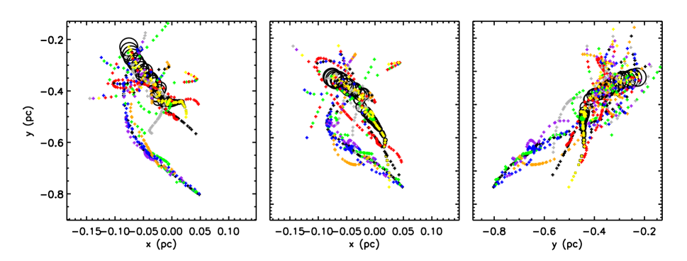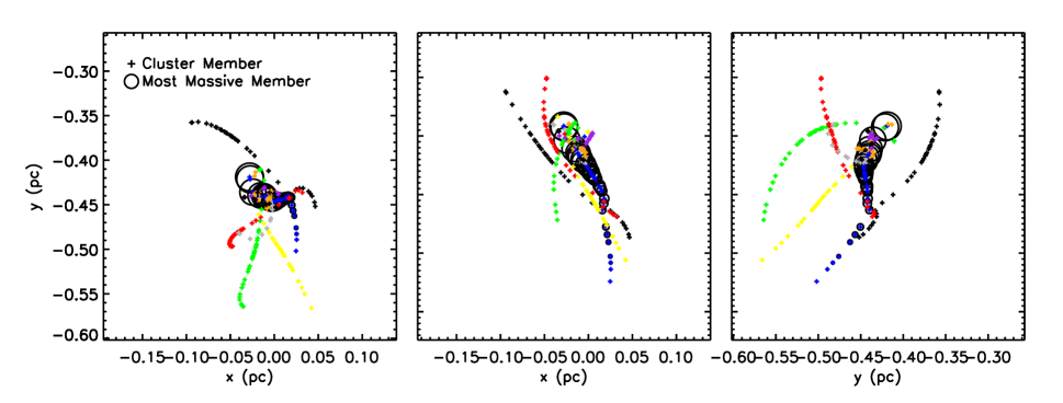
Figure 5 shows the projected positions of two clusters as a function of time for views along the $x$, $y$, and $z$ axes ($yz$, $xz$, and $xy$ projections). In these figures, we take the list of cluster members at a given time and projection and plot the 2D views of the cluster member positions sampled every 0.01 Myr. Cluster member positions are indicated by the coloured plus signs, while the most massive cluster member is shown with the circle, whose size scales with time. The direction of motion of the most massive member can be inferred by following the circle from small to larger sizes. The top panel shows a small cluster which only satisfied all MST cluster criteria for several time steps in the $xz$ projection. Several points can be taken from this plot: first, the three projected views have a fairly similar appearance, implying that many of the cluster members are indeed clustered in 3D space. Second, many of the stars remain clustered at early times in the simulation – the largest motion seen is the bulk motion of the entire group. The most massive cluster member moves very little with respect to the surrounding stars: only several lower mass stars have significant relative motions as they join (or are expelled from) the cluster.

The lower panel of Figure 5 shows a similar view for a larger cluster, identified in the $xz$ projection, which satisfied the MST cluster definition for a large fraction of the simulation in multiple views. These views are ‘messier’, showing greater interactions between cluster members. Despite this, the most massive cluster member usually appears near the middle of the stars, rather than moving there due to early dynamical interactions. Finally, note that this figure illustrates that (larger) clusters may include members which are only associated along the line of sight: in the bottom left panel of Figure 5, at earlier times (lower right of plot), there are clearly two highly separated groupings of stars (similar position in $x$ but not $y$), which appear as a single grouping in the middle plot (similar $x$ and $z$ at the lower right). Figure 5 also demonstrates that the cluster evolution proceeds without the merging of small clusters (e.g., Maschberger et al., 2010), although individual stars may join. The stellar densities in the simulations are sufficiently low that only 1 or 2 clusters are present at once, so it is unlikely for clusters to interact and merge.

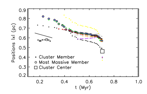
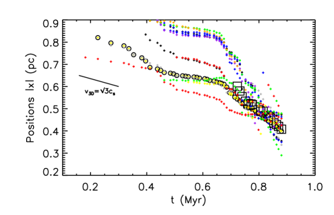
Rather than relying solely on projected views, we can also consider the full 3D picture at once. Figure 6 shows the root-mean-squared three-dimensional trajectory of the cluster members as a function of time for the same two clusters as shown in Figure 5. In this figure, the most massive cluster member’s 3D position is shown as a large circle at each time step, while other cluster members are indicated by small coloured plusses. At time steps when the stars meet our criteria for a cluster, a proxy for the 3D cluster center is shown by the square. In the upper panel, the stars only meet the MST cluster definition for a short time, while in the bottom panel, the cluster definition is satisfied for a longer period of time, although still less than half of the time in which stars have formed.

Several important points are quickly apparent from these figures. First, the most massive member typically forms early; see Section 4.5. Additional protostars which are eventually included in the MST-defined cluster form later, sometimes in close proximity to the most massive member and sometimes further away, migrating towards the position of the most massive member. Second, the motion of the most massive member is $\lesssim\sqrt{3}c_{s}$ and is relatively constant. This is significant because dynamical interactions between cluster members may “heat” up the velocities as the cluster becomes virialized (Proszkow & Adams, 2009). Finally, although cluster members do appear to be dynamically interacting (e.g., top panel Figure 6), the most massive member is already close to the MST-defined center often several $0.1$ Myr before a cluster is identified and before many close interactions occur.

Some 2D-defined clusters contain members not associated in 3D space. In Figure 6, this results in an offset of the three-dimensional center position relative to the most-massive member. Interestingly, these more distant members do not effect the conclusion that the protostars are primordially mass segregated. If anything, the random projected placement of these MST members would make the clusters appear less mass segregated than they actually are, by shifting the apparent cluster centre away from its true location. Observed mass-segregated clusters are thus likely to be more mass segregated than they appear due to the inclusion of unrelated stars due to chance alignments.

Figure 6: The three-dimensional position ($|{\bf x}|=\sqrt{x^{2}+y^{2}+z^{2}}$) of all cluster members for the same two clusters as in Figure 5. The most massive member is indicated by the black circles. The boxes show the cluster center computed from the MST. The line gives the trajectory for a particle moving with an rms velocity of $\sqrt{3}c_{\rm s}=0.35$ km s^-1.

4.5 Stellar Formation Times

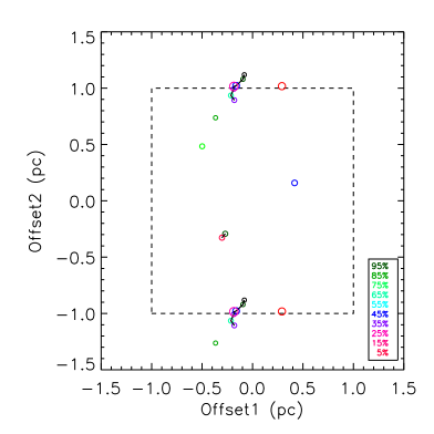
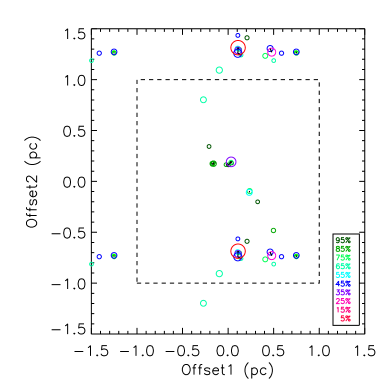
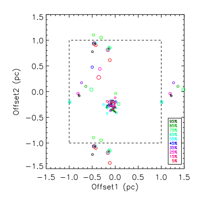
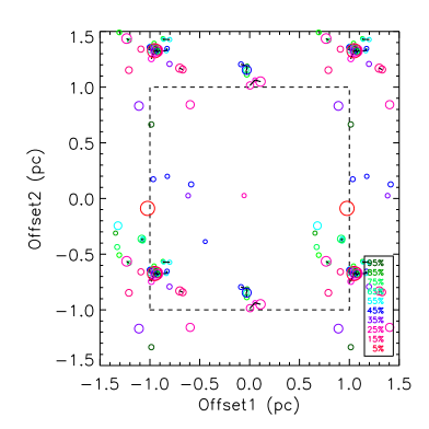
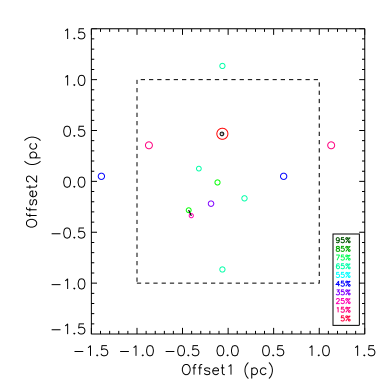
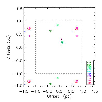
As noted in Section 4.4, the most massive member of each cluster tends to form early in the simulation. Figure 7 illustrates the relative formation times of the stars in the simulation, showing the final time step of each simulation except Rrt (excluded since it forms the fewest stars), viewed in the $xy$ projection. The stars are shown as the coloured circles, with the circle size scaling with mass, and the MST structure is shown with the black lines. The colours assigned to each star represent how early in the simulation they first formed: red and purple indicate earlier times, while green and light blue indicate later times, all calculated as the fraction of time elapsed since the first star formed in the simulation. What is immediately apparent from this figure is that the most massive stars all started forming early in the simulations – less than one third of the time since the first star formed. Some low mass stars also formed early, but other low mass stars continue to form throughout the simulation, as shown by the blue and green circles. In Rm6 and Rm6s, where MST clusters of more than ten members were identified using the best fit L_crit, the most massive star formed is a member of a cluster in at least one projection. This trend does not extend much further in the mass-ranking, however, in several instances somewhat massive stars appear to be associated with smaller (N$\leq$10 member) groups for at least some time steps. We emphasize that although the massive stars may start forming early, this does not imply that they also stop forming early. Since there is no stellar feedback included in the simulation, which could reduce or halt accretion, it is not surprising that stars continue to accrete. A longer formation time for higher mass stars is consistent with certain types of analytic accretion models in which accretion rates depend weakly or are independent of stellar mass (Bate & Bonnell, 2005; Myers, 2009; McKee & Offner, 2010). A tendency for more massive stars to begin forming early has also been noted in some previous simulations (e.g., Klessen 2001; Bate et al. 2003; Bonnell et al. 2004; Maschberger et al. 2010). Furthermore, Smith et al. (2009) find that the dense cores in which massive stars form out of tend form first as well.

Figure 7: The relative ages of stars formed in each of the simulations. For each simulation the $xy$ projection is shown at the final time step, with the same plotting convention for the stars and MST structure as previous figures, e.g., Figure 1. The colour assigned to each star indicates when it formed in the simulation as a fraction of the time elapsed since the first star in the simulation formed (see legend on bottom right); larger percentages thus indicate younger (more recently formed) stars. The simulations shown are, from left to right, top row: Rk34 and Rm4, middle row: Rm6 and Rm6s, bottom row: Rm9, Rt20. Rrt formed the fewest stars and is omitted for brevity.

5 Comparison with Observations

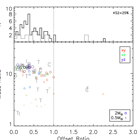
KM11 found in their observational survey of young, small, and nearby clusters, that the most massive cluster member tended to be centrally located (offset ratios of $<$1), with no dependence on other cluster properties, such as number of members, mass, or mass ratio. Figure 8 shows the mass and offset ratios found in the Rm6 clusters compared with those in the observational survey. In the lower panel of Figure 8, circles show the simulated clusters, with the circle size varying with the mass of the most massive cluster member, colour varying with projected view, and shading varying with the time, sampled every 0.01 Myr. The grey letters indicate the observed cluster values in KM11 for Taurus, Lupus3, ChaI, and IC348. The simulated clusters here clearly match the observations well – nearly all have offset ratios less than one, and similar, though smaller range of mass ratios. There is no trend in the offset ratio varying with the mass ratio or most massive cluster member’s mass. The histogram in the top panel of Figure 8 shows the distribution of offset ratios for both the simulation (black line) and observations (grey line) - both are similar. A KS test shows the probability that both observed and simulated offset distributions are drawn from the same parent sample is 25% (top right corner); the two distributions are clearly consistent.

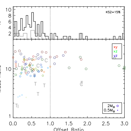
Figure 9 shows the comparable results for the Rm6s simulation, showing the same broad characteristics: the majority of offset ratios are much less than 1, and mass ratios around 10 to 20. Rm6s appears to have generally slightly higher mass ratios, and a broader distribution of offset ratios. The small differences between the two thus reflect the difference between the two random turbulent seeds.

None of the other simulations had any clusters with more than 10 members using their best-fit L_crit. Rm4 would have had a cluster identified at many time steps if a smaller minimum number of members were adopted for the cluster definition (e.g., $>5$ members). All of the other simulations require both a smaller minimum number of members and a larger L_crit in order for a cluster to be identified in more than one or two time steps and a single projection. We explore the effect of a more relaxed cluster definition in Appendix A.3, and find that the Rm6 and Rm6s clusters follow the same general behaviour as seen in Figure 8 and 9, and ‘clusters’ identified in the remaining simulations also behave similarly (see Figure 13). This implies that neither the specific cluster definition used nor the initial conditions has a strong influence on our results. At least in the regime of small-cluster formation, our results suggest an interesting conclusion. Changing the initial conditions in the simulation from the fiducial values which best match observations, to a larger or smaller Mach number, higher temperature, smaller turbulent driving scale, or including radiative effects has a significant impact on the number of stars formed, and their general clustering properties (stellar density, visual appearance, etc). Despite this, the most massive stars tend to form in what will become the centre of the cluster, suggesting that the mechanism for this is broadly applicable.

We note that the degree of mass segregation in local star-forming regions appears to be somewhat sensitive to how mass segregation is defined. For example, Parker et al. (2011) and Parker et al. (2012) do not find mass segregation in Taurus and $\rho-$Ophiuchi, respectively. In fact, Parker et al. (2011) claim to find inverse mass segregation in Taurus. These results initially appear to be in conflict with our MST analysis and the results of KM11, who also analyze Taurus, but the difference can be understood by comparing the two samples. Parker et al. (2011) include all the stars in their analysis, essentially assuming that the entire region behaves as one cluster, while KM11 make a point of identifying groupings within the sample, i.e., small-N analogs of higher mass clusters. We assert that subdivision is natural in regions such as Taurus, where star formation is distributed and stars in different areas appear to evolve with little knowledge of other subgroups.

Figure 8: The mass ratio and offset ratio for clusters identified in the Rm6 simulation, every 0.01 Myr, compared with observed cluster properties. Bottom panel: Red, green, and blue symbols show clusters identified for each projection, and lighter shades indicate earlier times in the simulation. The size of the circle indicates the mass of the most massive cluster member. The grey symbols indicate the ratios measured in KM11. Top panel: The distribution of offset ratios in the simulation (black) and from KM11 (grey). The probability that the two distributions are drawn from the same parent sample is given in the upper right corner. Randomly located most massive cluster members would lie around an offset ratio of 1 (dotted vertical line).

Figure 9: The mass and offset ratios for clusters in the Rm6s simulation every 0.01 Myr. See Figure 8 for the plotting conventions used.

6 Conclusions

Recent observations have shown that small stellar groupings of $\sim 10-40$ members and only 1-2 Myr old, have a centrally-located most massive member (Kirk & Myers, 2011), reminiscent of the mass segregation which is often claimed to be observed in larger, denser stellar clusters such as the Orion Nebula Cluster (Hillenbrand & Hartmann, 1998b). In both cases, this leads to the larger question of whether such mass segregation is primordial, or if it is a result of dynamical interactions between cluster members early in the cluster’s history. For large clusters, there is also debate about whether observational biases (e.g., from stellar crowding in the cluster centre) causes some or all of the apparent mass segregation (Ascenso et al., 2009). Even if the mass segregation is real, some amount of dynamical evolution is likely for larger clusters, since they tend to be both older and have smaller stellar interaction timescales. Observational bias is not present, however, for the small, sparse clusters in Kirk & Myers (2011), and here we verify that dynamical evolution is also unlikely to significantly impact or enhance mass segregation once a cluster has been identified.

Most previous simulations have focussed on higher density systems, where dynamical interactions are expected to play an important role in producing mass segregation. We analyze a suite of numerical simulations with varying initial conditions which form small clustered systems, in order to investigate the early dynamics of such systems. We examine the effect of variations in the Mach number, temperature, and driving scale on clustering, including one case which includes radiative transfer. We analyze the small stellar clusters formed in these simulations in the same manner as applied to the observations. At each time step, we “observe” the simulation from three viewing angles, removing the lower-mass companions in tight pairs which would be unresolved and any stars with masses below the completeness limit in Kirk & Myers (2011). We identify clusters using the minimal spanning tree (MST) formalism (e.g., Gutermuth et al., 2009), and then apply the same analyses as in Kirk & Myers (2011). Ours is the first study which applies the MST analysis to simulations in an identical manner to observational work, although Maschberger et al. (2010) and Girichidis et al. (2012) do apply an MST without observational cutoffs for their analysis.

Only the fiducial simulation and a second random realization of the same initial conditions result in clusters satisfying the observational requirements (more than 10 members connected in an MST by branch lengths of less than the locally-measured L_crit). Relaxing the observational requirements allows clusters in the other simulations to also be identified. In all cases, we find the simulated clusters mimic the observations: the most massive cluster member tends to be centrally located. We furthermore find that the most massive cluster member’s position within the cluster shows little to no evolution with time. ‘Mass segregation’, such as it can be observed in such small clusters, is primordial in the simulations. This agrees well with various other lines of evidence suggesting that dynamics do not play a significant role in small, young, stellar clusters. For example, observations of low-mass cores show that core relative motions are small compared to the local turbulent velocity (Kirk et al., 2007; André et al., 2007; Rosolowsky et al., 2008). Furthermore, dense core gas and envelope gas (as traced by, e.g., N₂H⁺ and C¹⁸O, respectively) also have similar line-of-sight velocities (Kirk et al., 2010). Both findings suggest that stars are not formed with initially ballistic motions relative to the surrounding gas. Some turbulent simulations are able to reproduce the observed low core-to-core velocity dispersions (Offner et al., 2008). Such simulations also demonstrate that protostellar velocities are initially subvirial relative to the gas (Offner et al., 2009). If stars inherit their motions from the dense gas and, consequently, are slow-moving, then mass segregation observed after 1-2 Myr in low-mass star forming regions is likely predominantly primordial. Observations of protostellar luminosities in local star forming regions find that brighter sources are preferentially located in higher protostellar density regions, which may indicate early mass segregation (Kryukova et al., 2012). This conclusion could also be confirmed by examining the distribution of core masses; assuming a one-to-one mapping between dense cores and protostars, mass segregation should then also be detectable at the dense core stage. Note, however, that in more clustered environments, individual dense cores become difficult to separate, and objects identified are likely to be multiple dense cores blended together, despite the fact that these composite objects may have a similar mass function to the IMF (Reid et al., 2010; Michel et al., 2011).

Finally, we note that there is a tendency for the most massive cluster member to form relatively early in the simulation. Maschberger et al. (2010) found a similar trend in their analysis of a numerical simulation of large cluster formation; there, they note that the most massive cluster member forms early, within subclusters that merge to form larger clustered systems. Having the most massive member starting to form early is perhaps not unexpected: it has the most mass to accrete, and therefore may need more time overall to do so (e.g., Myers, 2009).

Unlike the simulations we analyze, stars forming in high-stellar density regions likely undergo many interactions on a short time scale. Thus, our conclusions do not apply to massive star forming regions, which may evolve quite differently.

Appendix A Critical Length Determination

The analysis and results presented throughout this paper rely on the definition of a cluster adopted. Using the MST formalism, there are two parameters which control the identification of clusters: the critical length scale beyond which stars are not connected to a cluster, L_crit, and the minimum number of members to be classified as a cluster, $N_{min}$. For the simulations we analyze, L_crit has a greater influence on the clusters identified, because all of the clusters identified are small. $N_{min}$ therefore cannot be raised much above 11 for clusters to be identified in any simulation, and $N_{min}$ also cannot be lowered much below 11 before properties such as the cluster centre become difficult to measure. The effect of a lower $N_{min}$ is examined in more detail in Appendix A.3. In this section, we focus on the uncertainties associated with determining L_crit, and the impact of these on our results.

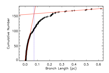
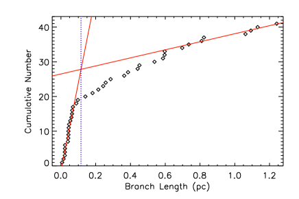
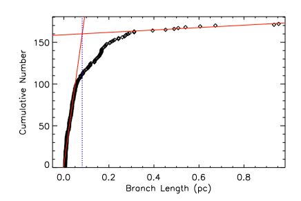
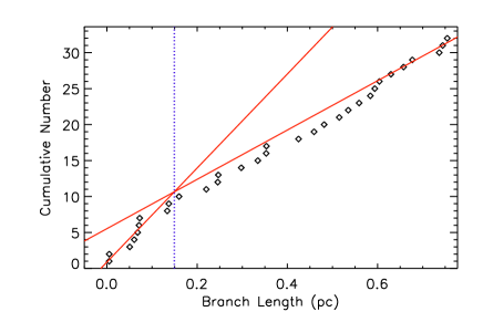
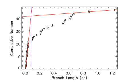
As discussed in Section 3, we determined L_crit following the procedure used in G09 and KM11. G09 found that MSTs in clustered star-forming regions tend to have a characteristic cumulative branch length distribution: a sharp, roughly linear rise at small lengths, followed by a turn-over, and a roughly linear shallow rise at large branch lengths. This is illustrated in Figure 10, showing the cumulative branch length distribution for the Rm6s simulation at the final timestep. G09 performed a linear fit to the steep and shallow slopes of the distribution, defining L_crit as the intersection between these two best-fit lines. This point gives an approximation of the turn-over location in the cumulative branch length distribution. We followed the same procedure in our analysis; the linear fits for Rm6s are shown in Figure 10. Note that while our full MSTs from the simulations contain the nine replications of the initial simulated box (to account for edge effects within the periodic boundaries), we took care to remove any duplicate branches prior to fitting. More accurate fits are obtained with a larger number of branches, and so we included all three projections at once for our critical length measurement. Examination of the branch length distribution for each projection separately revealed similar critical lengths when there were sufficient points for a good fit. Figure 11 shows the cumulative branch length distributions and L_crit determinations for the remaining six simulations. Qualitatively, many of the simulations have a markedly different shape to the cumulative branch length distribution than is observed – Rm6s appears the most similar to observed distributions, while simulations such as Rm9 are notably different, with too-steep slopes at both small and large branch lengths. This difference may be partially attributable to the small number of branches in several of the simulations, or it may be indicative of differences in the clustering properties.

Figure 10: The distribution of MST branch lengths for Rm6s. The red sold lines show the linear fits to the two edges of the distribution, and the blue dotted line shows the critical length measured, $\sim 0.07$ pc.

Figure 11: The distribution of MST branch lengths for all of the remaining simulations. Top row: Rk34, Rm4, middle row: Rm6, Rm9, and bottom row: Rt20, Rrt. The red solid lines show the linear fits to the two edges of the branch length distribution, and the blue dotted line shows the critical length measured. The critical lengths are given in Table 2.

A.1 Uncertainties

For cumulative branch length distributions where the slope of the steeper slope is not extreme, such as in Rm6s or Rm6, KM11 found that the uncertainty in L_crit is roughly 10%. In the case of the steepest branch length distributions (e.g., Rk34), the uncertainty in L_crit is likely larger. Examining the cumulative branch length distributions, however, also suggests that a change of that magnitude in L_crit will have a relatively minor impact on the clusters identified. Moving the dashed blue L_crit line in Figures 10 and 11 by 10% or even 20% does not result in a large change in the cumulative number (vertical axis) of MST branches which could be connecting stars in a cluster. This is an upper limit to the number of stars whose cluster membership would start (end) with the increase (decrease) in L_crit; some of the stars indicated by these points would be associated with groupings of stars which are too small to meet the minimum cluster size. Only a few stars at a cluster’s periphery are therefore likely to change their cluster membership status within reasonable variations of L_crit. KM11 found similar results in their observational survey.

A.2 Time Evolution

The cumulative branch length distributions shown in Figures 10 and 11 are all from the final time step that each simulation was run. In principle, a similar analysis should be made at each time step for each simulation. Where the number of branches was sufficiently large to perform accurate fits, we searched for evidence of time evolution of L_crit or the shape of the cumulative branch length distribution. For Rm9 and Rrt, too few sources were ever present to allow for a good determination of L_crit, as noted in Table 2. For Rk34 and Rt20, the paucity of sources, particularly at earlier time steps, was sufficient to lead to a $>$10% scatter in L_crit, although the general shape of the cumulative branch length distribution does not change significantly after the first few time steps examined. For Rm4, Rm6, and Rm6s, which had the greatest number of sources, the overall shape of the cumulative branch length distribution appears to change little over time. There is some variation in the values of the L_crit fit, but no definitive evidence for systematic increase or decrease in L_crit with time. At the earliest times when the number of sources is smallest, both the shape of the cumulative branch length distribution and the fit L_crit tends to be more variable, often appearing more similar to, e.g., the Rm9 distribution in Figure 11. At the time steps examined, L_crit for Rm6 tended to lie between 0.06 pc and 0.08 pc, although in a few cases, the best fit values had more extreme values (between 0.05 pc and 0.09 pc to 0.1 pc). Rm6s showed a slightly larger scatter in L_crit values, but similarly most values were between 0.06 pc and 0.08 pc.

Given these findings, we argue it is reasonable to adopt a single, constant value of L_crit for each simulation; there is no strong evidence for evolution of L_crit with time which might potentially bias our results. In Appendix A.3 we further demonstrate that our results are robust to the precise L_crit adopted; we find similar results even when L_crit is increased beyond the uncertainty discussed here.

A.3 Maximal Cluster Membership

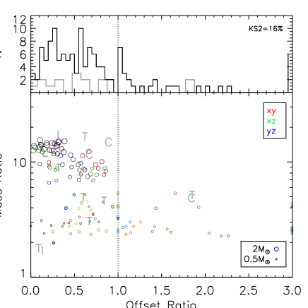
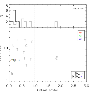
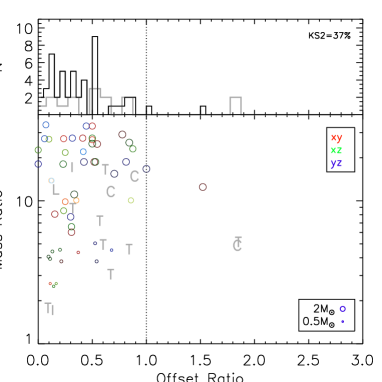
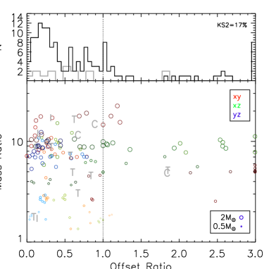
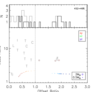
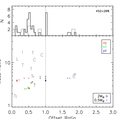
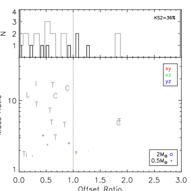
To further test the effects of our cluster definition on our results, we re-run the analysis shown in Section 5 with a more inclusive cluster definition. We change our cluster definition to a minimum of 6 stars (from 11). When a cluster has few stars, the centre position is poorly defined, generating a larger scatter in the offset ratios measured. We also increase L_crit to the maximum allowable before all stars in the simulation are connected in a single cluster, 0.15 pc for Rm4, Rm6, Rm6s, and Rrt, 0.3 pc for Rt20, and 0.5 pc for Rk34 and Rm9; these are at least 50% larger than the best fit values for each. [Note that since the simulations have periodic boundary conditions, defining the cluster centre would become problematic if all stars belong to the same cluster.]

Figures 12 and 13 show the resulting mass and offset ratios. In order to increase the amount of data available to plot, the 0.01 Myr time sampling has only been applied to Rm4, Rm6, and Rm6s; for the other simulations, all time steps are displayed. For Rm6 and Rm6s, these figures can be compared directly to their counterparts in Figures 8 and 9. Despite the substantial change in L_crit, as well as allowing clusters to be up to half as small, it is clear that the results are qualitatively similar. For both cluster definitions, the majority of offset ratios are less than 1, and the distributions are consistent with the observed clusters. The mass ratios extend to smaller values with the maximally inclusive cluster definition, since the smallest, sparsest, ‘clusters’ now added to the sample tend to lack the more massive stars present in the original cluster sample.

After Rm6 and Rm6s, Rm4 produces the most clusters, and clearly follows a similar trend to the former. The remaining simulations, despite the extremely relaxed cluster criteria adopted, still form very few clusters. Most of these have offset ratios of less than one. The one exception is Rm9, which appears equally split between offset ratios below and above one. Here, only two clusters were identified (one each in the xy and yz projections). Both groupings are small, and sufficiently sparse that they would likely not have been visually selected as clusters. Most of the identified members have similarly small masses, which is a regime in which the offset ratios could be expected to be random. In the $xy$ projection (red points), at early times, a more massive star is separated by just under 0.5 pc from the cluster outskirts, leading to the larger offset and mass ratios, both of which drop significantly when that star drifts slightly further away.

Figure 12: The mass and offset ratio for clusters identified in the Rm6 simulation, with the value of $L_{crit}$ increased to 0.15 pc from 0.07 pc, and the minimum number of members required to be classified as a cluster reduced to 6 (from 11). Clusters with offset ratios of more than 3 are all plotted as having a value of precisely 3. The same trends are followed as in Figure 8 are found for this relaxed cluster definition. See Figure 8 for the plotting conventions used.

Figure 13: The mass and offset ratios for clusters identified with relaxed cluster definitions. Top row: Rk34 and Rm4, middle row: Rm6s and Rm9, bottom row: Rt20 and Rrt with L_crit values of 0.5, 0.15, 0.15, 0.5, 0.5, and 0.15 pc respectively, and a minimum of 6 members required. Clusters with offset ratios above 3 are plotted with a value of 3. For all simulations except Rm4 and Rm6s, all time slices in the simulation are included to increase the total number of data points. See Figure 8 for the plotting conventions used.

Appendix B Cluster Centre Definition

The ratio of the offset of the most massive cluster member from the centre to the median cluster member offset, the offset ratio, is influenced by one factor in addition to the cluster definition examined in Appendix A, the definition of the cluster’s centre. We demonstrate here that this does not strongly influence on our results.

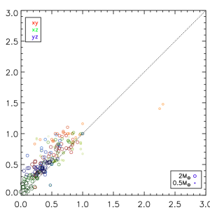
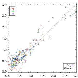
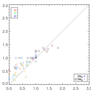
Following KM11, in our main analysis, we adopt the median cluster position as the centre, as the median is less influenced than the mean by outliers in small-number samples. Here, we show the effect of instead adopting the mean position for the centre. Figure 14 shows a comparison of the offset ratios measured using the median- and mean-determined centres, using L_crit from Table 2 and $N_{min}$ of 11 for Rm6 and Rm6s, and 6 for Rm4. Figure 14 shows significant scatter between the two offset ratios, but no tendency for the mean-determined offset ratio to be systematically higher than the median-determined offset ratio (points lying preferentially below the dashed line in Figure 14 ). Instead, any bias appears to be in the opposite direction, i.e., with a mean-defined cluster centre, we would have found preferentially lower offset ratios. The small excess of offset ratios of 1 is from clusters with an odd number of members, whose most massive member has an offset ratio at precisely the middle of the range of offset ratios.

Finally, we note that using the centre of mass of the cluster to define its centre, there would more strongly tend to give small offset ratios, since the central position would be biassed toward the location of the most massive cluster member. Our finding that the most massive cluster member tends to form (and remain) in the cluster centre is therefore robust to any reasonable variation imposed on the definition of a cluster (previous section) and its centre (this section).

Figure 14: A comparison of the offset ratios derived assuming the cluster centre is the median or mean cluster member position. From left to right: Rm6, Rm6s, and Rm4. The dashed line denotes a 1-1 relationship. As in Figure 8, the colours denote the projection in which the simulations are being viewed, the shading scales with the cluster’s evolution in time, and the size of the symbols scales with the mass of the most massive cluster member.

References

- Allison et al. (2009) Allison R. J., Goodwin S. P., Parker R. J., de Grijs R., Portegies Zwart S. F., Kouwenhoven M. B. N., 2009, ApJL, 700, L99
- Allison et al. (2009) Allison R. J., Goodwin S. P., Parker R. J., Portegies Zwart S. F., de Grijs R., Kouwenhoven M. B. N., 2009, MNRAS, 395, 1449
- Alves et al. (2007) Alves J., Lombardi M., Lada C. J., 2007, A&A, 462, L17
- André et al. (2007) André P., Belloche A., Motte F., Peretto N., 2007, A&A, 472, 519
- Ascenso et al. (2009) Ascenso J., Alves J., Lago M. T. V. T., 2009, A&A, 495, 147
- Barrow et al. (1985) Barrow J. D., Bhavsar S. P., Sonoda D. H., 1985, MNRAS, 216, 17
- Bastian et al. (2010) Bastian N., Covey K. R., Meyer M. R., 2010, ARA&A, 48, 339
- Bate (2009) Bate M. R., 2009, MNRAS, 392, 1363
- Bate (2012) Bate M. R., 2012, MNRAS, 419, 3115
- Bate & Bonnell (2005) Bate M. R., Bonnell I. A., 2005, MNRAS, 356, 1201
- Bate et al. (2003) Bate M. R., Bonnell I. A., Bromm V., 2003, MNRAS, 339, 577
- Bonnell et al. (1997) Bonnell I. A., Bate M. R., Clarke C. J., Pringle J. E., 1997, MNRAS, 285, 201
- Bonnell et al. (2001) Bonnell I. A., Bate M. R., Clarke C. J., Pringle J. E., 2001, MNRAS, 323, 785
- Bonnell & Davies (1998) Bonnell I. A., Davies M. B., 1998, MNRAS, 295, 691
- Bonnell et al. (2004) Bonnell I. A., Vine S. G., Bate M. R., 2004, MNRAS, 349, 735
- Bressert et al. (2010) Bressert E., Bastian N., Gutermuth R., Megeath S. T., Allen L., Evans II N. J., Rebull L. M., Hatchell J., Johnstone D., Bourke T. L., Cieza L. A., Harvey P. M., Merin B., Ray T. P., Tothill N. F. H., 2010, MNRAS, 409, L54
- Cartwright & Whitworth (2004) Cartwright A., Whitworth A. P., 2004, MNRAS, 348, 589
- Commerçon et al. (2011) Commerçon B., Hennebelle P., Henning T., 2011, ApJL, 742, L9
- Conover (1999) Conover W. J., 1999, Practical Nonparametric Statistics, 3rd edn. Wiley, New York
- Delgado-Donate et al. (2003) Delgado-Donate E. J., Clarke C. J., Bate M. R., 2003, MNRAS, 342, 926
- Gieles et al. (2012) Gieles M., Moeckel N., Clarke C. J., 2012, MNRAS, 426, L11
- Girichidis et al. (2012) Girichidis P., Federrath C., Allison R., Banerjee R., Klessen R. S., 2012, MNRAS, 420, 3264
- Girichidis et al. (2011) Girichidis P., Federrath C., Banerjee R., Klessen R. S., 2011, MNRAS, 413, 2741
- Gouliermis et al. (2004) Gouliermis D., Keller S. C., Kontizas M., Kontizas E., Bellas-Velidis I., 2004, A&A, 416, 137
- Gutermuth et al. (2009) Gutermuth R. A., Megeath S. T., Myers P. C., Allen L. E., Pipher J. L., Fazio G. G., 2009, ApJS, 184, 18
- Hillenbrand & Hartmann (1998a) Hillenbrand L. A., Hartmann L. W., 1998a, ApJ, 492, 540
- Hillenbrand & Hartmann (1998b) Hillenbrand L. A., Hartmann L. W., 1998b, ApJ, 492, 540
- Jørgensen et al. (2008) Jørgensen J. K., Johnstone D., Kirk H., Myers P. C., Allen L. E., Shirley Y. L., 2008, ApJ, 683, 822
- Kirk et al. (2007) Kirk H., Johnstone D., Tafalla M., 2007, ApJ, 668, 1042
- Kirk & Myers (2011) Kirk H., Myers P. C., 2011, ApJ, 727, 64
- Kirk et al. (2010) Kirk H., Pineda J. E., Johnstone D., Goodman A., 2010, ApJ, 723, 457
- Klein (1999) Klein R. I., 1999, Journal of Computational and Applied Mathematics, 109, 123
- Klessen (2001) Klessen R. S., 2001, ApJ, 556, 837
- Krumholz et al. (2007) Krumholz M. R., Klein R. I., McKee C. F., 2007, ApJ, 656, 959
- Krumholz et al. (2012) Krumholz M. R., Klein R. I., McKee C. F., 2012, ApJ, 754, 71
- Krumholz et al. (2004) Krumholz M. R., McKee C. F., Klein R. I., 2004, ApJ, 611, 399
- Kryukova et al. (2012) Kryukova E., Megeath S. T., Gutermuth R. A., Pipher J., Allen T. S., Allen L. E., Myers P. C., Muzerolle J., 2012, AJ, 144, 31
- Lada & Lada (2003) Lada C. J., Lada E. A., 2003, ARA&A, 41, 57
- Luhman et al. (2009) Luhman K. L., Mamajek E. E., Allen P. R., Cruz K. L., 2009, ApJ, 703, 399
- Maschberger & Clarke (2011) Maschberger T., Clarke C. J., 2011, MNRAS, 416, 541
- Maschberger et al. (2010) Maschberger T., Clarke C. J., Bonnell I. A., Kroupa P., 2010, MNRAS, 404, 1061
- Masiunas et al. (2012) Masiunas L. C., Gutermuth R. A., Pipher J. L., Megeath S. T., Myers P. C., Allen L. E., Kirk H. M., Fazio G. G., 2012, ApJ, 752, 127
- McKee & Offner (2010) McKee C. F., Offner S. S. R., 2010, ApJ, 716, 167
- McKee & Ostriker (2007) McKee C. F., Ostriker E. C., 2007, ARA&A, 45, 565
- Meylan & Heggie (1997) Meylan G., Heggie D. C., 1997, A&A Rev., 8, 1
- Michel et al. (2011) Michel M., Kirk H., Myers P. C., 2011, ApJ, 735, 51
- Myers (2009) Myers P. C., 2009, ApJ, 706, 1341
- Offner et al. (2013) Offner S. S. R., Bisbas T. G., Viti S., Bell T. A., 2013, ApJ, 770, 49
- Offner et al. (2009) Offner S. S. R., Hansen C. E., Krumholz M. R., 2009, ApJL, 704, L124
- Offner et al. (2008) Offner S. S. R., Klein R. I., McKee C. F., 2008, ApJ, 681, 375
- Offner et al. (2009) Offner S. S. R., Klein R. I., McKee C. F., Krumholz M. R., 2009, ApJ, 703, 131
- Offner et al. (2008) Offner S. S. R., Krumholz M. R., Klein R. I., McKee C. F., 2008, AJ, 136, 4040
- Parker et al. (2011) Parker R. J., Bouvier J., Goodwin S. P., Moraux E., Allison R. J., Guieu S., Güdel M., 2011, MNRAS, 412, 2489
- Parker et al. (2012) Parker R. J., Maschberger T., Alves de Oliveira C., 2012, MNRAS, 426, 3079
- Parker & Meyer (2012) Parker R. J., Meyer M. R., 2012, MNRAS, 427, 637
- Parker et al. (2013) Parker R. J., Wright N. J., Goodwin S. P., Meyer M. R., 2013, ArXiv e-prints
- Proszkow & Adams (2009) Proszkow E.-M., Adams F. C., 2009, ApJS, 185, 486
- Reid et al. (2010) Reid M. A., Wadsley J., Petitclerc N., Sills A., 2010, ApJ, 719, 561
- Rosolowsky et al. (2008) Rosolowsky E. W., Pineda J. E., Foster J. B., Borkin M. A., Kauffmann J., Caselli P., Myers P. C., Goodman A. A., 2008, ApJS, 175, 509
- Smith et al. (2009) Smith R. J., Clark P. C., Bonnell I. A., 2009, MNRAS, 396, 830
- Solomon et al. (1987) Solomon P. M., Rivolo A. R., Barrett J., Yahil A., 1987, ApJ, 319, 730
- Spitzer (1969) Spitzer Jr. L., 1969, ApJL, 158, L139
- Truelove et al. (1997) Truelove J. K., Klein R. I., McKee C. F., Holliman II J. H., Howell L. H., Greenough J. A., 1997, ApJL, 489, L179+
- Truelove et al. (1998) Truelove J. K., Klein R. I., McKee C. F., Holliman II J. H., Howell L. H., Greenough J. A., Woods D. T., 1998, ApJ, 495, 821
- Weidner et al. (2010) Weidner C., Kroupa P., Bonnell I. A. D., 2010, MNRAS, 401, 275