Embedding Graphs under Centrality Constraints for Network Visualization

Abstract

Visual rendering of graphs is a key task in the mapping of complex network data. Although most graph drawing algorithms emphasize aesthetic appeal, certain applications such as travel-time maps place more importance on visualization of structural network properties. The present paper advocates two graph embedding approaches with centrality considerations to comply with node hierarchy. The problem is formulated first as one of constrained multi-dimensional scaling (MDS), and it is solved via block coordinate descent iterations with successive approximations and guaranteed convergence to a KKT point. In addition, a regularization term enforcing graph smoothness is incorporated with the goal of reducing edge crossings. A second approach leverages the locally-linear embedding (LLE) algorithm which assumes that the graph encodes data sampled from a low-dimensional manifold. Closed-form solutions to the resulting centrality-constrained optimization problems are determined yielding meaningful embeddings. Experimental results demonstrate the efficacy of both approaches, especially for visualizing large networks on the order of thousands of nodes.

1 Introduction

Graphs offer a valuable means of encoding relational information between entities of complex systems, arising in modern communications, transportation and social networks, among others [1], [2]. Although graph embedding serves a number of tasks including data compression and a means to geometrically solve computationally hard tasks, information visualization remains its most popular application. However, the rising complexity and volume of networked data presents new opportunities and challenges for visual analysis tools that capture global patterns and use visual metaphors to convey meaningful structural information like hierarchy, similarity and natural communities [13].

Most traditional visualization algorithms trade-off the clarity of structural characteristics of the underlying data for aesthetic requirements like minimal edge crossing and fixed inter-node distance; e.g., [6, 8, 14, 15, 16, 17, 18, 19, 20]. Although efficient for relatively small graphs (hundreds of nodes), embeddings for larger graphs using these techniques are seldom structurally informative. To this end, several approaches have been developed for embedding graphs while preserving specific structural properties.

Pioneering methods (e.g. [33]) have resorted to MDS, which seeks a low-dimensional depiction of high-dimensional data in which pairwise Euclidean distances between embedding coordinates are close (in a well-defined sense) to the dissimilarities between the original data points [31], [38]. In this case, the vertex dissimilarity structure is preserved through pairwise distance metrics between vertices.

Principal component analysis (PCA) of the graph adjacency matrix is advocated in [3], leading to a spectral embedding whose vertices correspond to entries of the leading component vectors. The structure preserving embedding algorithm [4] solves a semidefinite program with linear topology constraints so that a nearest neighbor algorithm can recover the graph edges from the embedding.

Visual analytics approaches developed in [7] and [12] emphasize community structures with applications to community browsing in graphs. Concentric graph layouts developed in [39] and [30] capture notions of node hierarchy by placing the highest ranked nodes at the center of the embedding.

Although the graph embedding problem has been studied for years, development of fast and optimal visualization algorithms with hierarchical constraints is challenging and existing methods typically resort to heuristic approaches. The growing interest in analysis of very large networks has prioritized the need for effectively capturing hierarchy over aesthetic appeal in visualization. For instance, a hierarchy-aware visual analysis of a global computer network is naturally more useful to security experts trying to protect the most critical nodes from a viral infection. Layouts of metro-transit networks that clearly show terminals routing the bulk of traffic convey a better picture about the most critical nodes in the event of a terrorist attack.

In this paper, hierarchy is captured through well-defined measures of node importance collectively known as centrality in the network science community (see e.g.,  [22], [23]). For instance, betweenness centrality describes the extent to which information is routed through a specific node by measuring the fraction of all shortest paths traversing it; see e.g., [1, p. 89]. Other measures include closeness, eigenvalue, and Markov centrality. Motivated by the desire for more effective approaches to capture centrality structure, dimensionality reduction techniques are leveraged to develop graph embedding algorithms that adhere to hierarchy.

1.1 Contributions

The present paper incorporates centrality structure by explicitly constraining MDS and LLE embedding criteria and developing efficient algorithms that yield structurally informative visualizations. First, an MDS (so-termed stress [31, Chap. 3]) optimization criterion with radial constraints that place nodes of higher centrality closer to the origin of the graph embedding is adopted. The novel approach exploits the block separability inherent to the proposed model and introduces successive approximations to determine the optimal embedding via coordinate descent iterations. In addition, edge crossings are minimized by regularizing the stress cost with a smoothness promoting term weighted by a tuning parameter.

The second approach develops a centrality-constrained LLE visualization algorithm. Closed-form solutions for the weight determination step and low-complexity coordinate descent iterations for the dimensionality reduction step are developed yielding a fast algorithm that scales linearly with the graph size. Moreover, the LLE approach inherently preserves local structure under centrality constraints eliminating the need for a smoothness regularization penalty.

1.2 Related work

Although the graph embedding problem has generally been studied for some time, the use of centralities to guide visualization is recent and has been addressed predominantly in the context of scale-free networks. The derivatives of centrality metrics [5] are used to visualize social networks in a way that captures the sensitivity of nodes to changes in degree of a given node. Edge filtering based on betweenness centrality is used by [9] to improve the layout of large graphs. Similar filtering approaches in [10] and [11] remove edges with high betweenness centrality leading to clearer layouts that capture the structure of the network.

Closer to the objectives of the present paper is work involving radial visualizations [30] generated by iteratively solving an MDS stress function with centrality-based weights. However, the proposed algorithm is sensitive to initialization and offers no convergence guarantee, a limitation that is addressed in this paper. In another study whose results have been used extensively for internet visualization, the $k$-core decomposition is used to hierarchically place nodes within concentric “onion-like” shells [39]. Although effective for large-scale networks, it is a heuristic method with no optimality associated with it.

1.3 Structure of the paper

The rest of this paper is organized as follows. Section 2 states the graph embedding problem and Section 3 casts it as MDS with centrality constraints. BCD iterations are used to solve the MDS problem in Section 4 and a smoothness penalty is included in Section 5. Section 6 solves the embedding problem via LLE, whereas Sections 7 and 8 discuss centrality measures and node dissimilarities relevant as inputs to the proposed algorithms respectively. Experimental results are presented in Section 9, and concluding remarks are given in Section 10.

Notation. Upper (lower) bold face letters denote matrices (column vectors) and calligraphic letters denote sets; ${\mathbf{X}}^{T}$ denotes transpose of ${\mathbf{X}}$; $\text{Tr}\left({\mathbf{X}}\right)$ is the trace operator of matrix ${\mathbf{X}}$; $\|{\mathbf{x}}\|_{2}$ is the Euclidean norm of ${\mathbf{x}}$; ${\mathbf{e}}_{i}$ is the $i$-th column of the identity matrix, $\mathbf{I}$. ${\mathbf{X}}_{\mathcal{I},\mathcal{J}}$ is the submatrix of ${\mathbf{X}}$ obtained by retaining the common elements in rows indexed by the elements of $\mathcal{I}$ and columns indexed by $\mathcal{J}$. Lastly, $\partial f(.)$ denotes the subdifferential of $f(.)$.

2 Preliminaries

Consider a network represented by a graph $\mathcal{G}=(\mathcal{V},\mathcal{E})$, where $\mathcal{E}$ denotes the set of edges, and $\mathcal{V}$ the set of vertices with cardinality $|\mathcal{V}|=N$. It is assumed that $\mathcal{G}$ is undirected, unweighted and has no loops or multi-edges between node pairs. Let $\delta_{ij}$ denote the real-valued pairwise dissimilarity between two nodes $i$ and $j$ computed via a well-defined criterion. The dissimilarities are assumed to satisfy the following properties: (i) $\delta_{ij}\geq 0$; (ii) $\delta_{ij}=\delta_{ji}$; and, (iii) $\delta_{ii}=0$. Consequently, it suffices to know the set $\mathcal{D}:=\{\{\delta_{ij}\}_{j=1}^{N}\}_{i=j+1}^{N}$ with cardinality $|\mathcal{D}|=N(N-1)/2$. Let $c_{i}$ denote a centrality measure assigned to node $i$, and consider the set $\mathcal{C}:=\{c_{i}\}_{i=1}^{N}$ with cardinality $|\mathcal{C}|=N$. Node centralities can be obtained using a number of algorithms [1, Chap. 4].

Given $\mathcal{G}$, $\mathcal{D}$, $\mathcal{C}$, and the prescribed embedding dimension $p$ (typically $p\in\{2,3\}$), the graph embedding task amounts to finding the set of $p\times 1$ vectors $\mathcal{X}:=\left\{{\mathbf{x}}_{i}\right\}_{i=1}^{N}$ which “respect” the network structure characteristics encoded through $\mathcal{D}$ and $\mathcal{C}$. The present paper puts forth two approaches, based upon dimensionality reduction, which ensure that $\mathcal{X}$ adheres to these constraints from different but related viewpoints.

3 Centrality-constrained MDS

MDS amounts to finding vectors $\left\{{\mathbf{x}}_{i}\right\}_{i=1}^{N}$ so that the embedding coordinates ${\mathbf{x}}_{i}$ and ${\mathbf{x}}_{j}$ satisfy $\|{\mathbf{x}}_{i}-{\mathbf{x}}_{j}\|_{2}\approx\delta_{ij}$ by solving the following problem:

$$(\text{P}0)\;\;\;\;\hat{\mathcal{X}}=\underset{{\mathbf{x}}_{1},\dots,{\mathbf{x}}_{N}}{\operatorname{arg\,min}}\text{ }\frac{1}{2}\sum_{i=1}^{N}\sum_{j=1}^{N}[\left\|\mathbf{x}_{i}-\mathbf{x}_{j}\right\|_{2}-\delta_{ij}]^{2}.$$ (1)

Centrality structure will be imposed on (1) by constraining ${\mathbf{x}}_{i}$ to have a centrality-dependent radial distance $f(c_{i})$, where $f(.)$ is a monotone decreasing function. For instance, $f(c_{i})=\alpha e^{-\beta c_{i}}$ where $\alpha$ and $\beta$ are positive constants. The resulting constrained optimization problem now becomes

$$(\text{P}1)\;\;\;\;\hat{\mathcal{X}}=\underset{{\mathbf{x}}_{1},\dots,{\mathbf{x}}_{N}}{\operatorname{arg\,min}} \frac{1}{2}\sum\limits_{i=1}^{N}\sum\limits_{j=1}^{N}\left[\left\|\mathbf{x}_{i}-\mathbf{x}_{j}\right\|_{2}-\delta_{ij}\right]^{2}$$

s. to $$\left\|\mathbf{x}_{i}\right\|_{2}=f(c_{i}),\text{ }i=1,\dots,N.$$ (2)

Although $\text{P}0$ is non-convex, standard solvers rely on gradient descent iterations but have no guarantees of convergence to the global optima [49]. Lack of convexity is exacerbated in $\text{P}1$ by the non-convex constraint set rendering its solution even more challenging than that of $\text{P}0$. However, considering a single embedding vector ${\mathbf{x}}_{i}$, and fixing the rest $\{{\mathbf{x}}_{j}\}_{j\neq i}$, the constraint set simplifies to $\|{\mathbf{x}}_{i}\|_{2}=f(c_{i})$, for which an appropriate relaxation can be sought. Key to the algorithm proposed next lies in this inherent decoupling of the centrality constraints.

Remark 1.

A number of stress costs with well-documented merits have been reported for MDS. The choice made in $P0$ is motivated by convenience of adaptation to BCD iterations discussed in Section 4. Moreover, more general forms include weights, which have been ignored without loss of generality.

4 BCD successive approximations

By exploiting the separable nature of the cost as well as the norm constraints in (3), BCD will be developed in this section to arrive at a solution approaching the global optimum. To this end, the centering constraint $\sum_{i=1}^{N}{\mathbf{x}}_{i}={\bf 0}$, typically invoked to fix the inherent translation ambiguity, will be dropped first so that the problem remains decoupled across nodes. The effect of this relaxation can be compensated for by computing the centroid of the solution of (3), and subtracting it from each coordinate. The $N$ equality norm constraints are also relaxed to $\|{\mathbf{x}}_{i}\|_{2}\leq f(c_{i})$. Although the entire constraint set is non-convex, each relaxed constraint is a convex and closed Euclidean ball with respect to each node in the network.

Let ${\mathbf{x}}_{i}^{r}$ denote the minimizer of the optimization problem over block $i$, when the remaining blocks $\left\{{\mathbf{x}}_{j}\right\}_{j\neq i}$ are fixed during the BCD iteration $r$. By fixing the blocks $\left\{{\mathbf{x}}_{j}\right\}_{j\neq i}$ to their most recently updated values, the sought embedding is obtained as

$$\hat{{\mathbf{x}}}_{i} = \underset{{\mathbf{x}}}{\operatorname{arg\,min}}\frac{1}{2}\sum_{j\neq i}\left[\left\|\mathbf{x}-\mathbf{x}_{j}\right\|_{2}-\delta_{ij}\right]^{2}$$

s. to $$\left\|\mathbf{x}\right\|_{2}\leq f(c_{i})$$ (3)

or equivalently as

$$\underset{{\mathbf{x}}}{\arg\min} \frac{(N-1)}{2}\|{\mathbf{x}}\|_{2}^{2}-{\mathbf{x}}^{T}(\sum_{j<i}{\mathbf{x}}_{j}^{r}+\sum_{j>i}{\mathbf{x}}_{j}^{r-1})$$

$$-\sum_{j<i}\delta_{ij}\|{\mathbf{x}}-{\mathbf{x}}_{j}^{r}\|_{2}-\sum_{j>i}\delta_{ij}\|{\mathbf{x}}-{\mathbf{x}}_{j}^{r-1}\|_{2}$$

s. to $$\left\|{\mathbf{x}}\right\|_{2}\leq f(c_{i})$$ (4)

where $\sum_{j<i}(.):=\sum_{j=1}^{i-1}(.)$ and $\sum_{j>i}(.):=\sum_{j=i+1}^{N}(.)$. With the last two sums in the cost function of (4) being non-convex and non-smooth, convergence of the BCD algorithm cannot be guaranteed [45, p. 272]. Moreover, it is desired to have each per-iteration subproblem solvable to global optimality, in closed form and at a minimum computational cost. The proposed approach seeks a global upper bound of the objective with the desirable properties of smoothness and convexity. To this end, consider the function $\Psi({\mathbf{x}}):=\psi_{1}({\mathbf{x}})-\psi_{2}({\mathbf{x}})$, where

$$\psi_{1}({\mathbf{x}}):=\frac{(N-1)}{2}\|{\mathbf{x}}\|_{2}^{2}-{\mathbf{x}}^{T}(\sum\limits_{j<i}{\mathbf{x}}_{j}^{r}+\sum\limits_{j>i}{\mathbf{x}}_{j}^{r-1})$$ (5)

and

$$\psi_{2}({\mathbf{x}}):=\sum\limits_{j<i}\delta_{ij}\|{\mathbf{x}}-{\mathbf{x}}_{j}^{r}\|_{2}+\sum\limits_{j>i}\delta_{ij}\|{\mathbf{x}}-{\mathbf{x}}_{j}^{r-1}\|_{2}.$$ (6)

Note that $\psi_{1}({\mathbf{x}})$ is a convex quadratic function, and that $\psi_{2}({\mathbf{x}})$ is convex (with respect to ${\mathbf{x}}$) but non-differentiable. The first-order approximation of (6) at any point in its domain is a global under-estimate of $\psi_{2}({\mathbf{x}})$. Despite the non-smoothness at some points, such a lower bound can always be established using its subdifferential. As a consequence of the convexity of $\psi_{2}({\mathbf{x}})$, it holds that [45, p. 731]

$$\psi_{2}({\mathbf{x}})\geq\psi_{2}({\mathbf{x}}_{0})+\mathbf{g}^{T}({\mathbf{x}}_{0})({\mathbf{x}}-{\mathbf{x}}_{0}),\forall{\mathbf{x}}\in\text{dom}(\psi_{2})$$ (7)

where $\mathbf{g}({\mathbf{x}})\in\partial\psi_{2}({\mathbf{x}})$ is a subgradient within the subdifferential set, $\partial\psi_{2}({\mathbf{x}})$ of $\psi_{2}({\mathbf{x}})$. The subdifferential of $\|{\mathbf{x}}-{\mathbf{x}}_{j}\|_{2}$ with respect to ${\mathbf{x}}$ is given by

$$\partial_{{\mathbf{x}}}\|{\mathbf{x}}-{\mathbf{x}}_{j}\|_{2}=\begin{cases}\frac{{\mathbf{x}}-{\mathbf{x}}_{j}}{\|{\mathbf{x}}-{\mathbf{x}}_{j}\|_{2}},&\text{ if }{\mathbf{x}}\neq{\mathbf{x}}_{j}\\ \mathbf{s}\in\mathbb{R}^{p}:\text{ }\|\mathbf{s}\|_{2}\leq 1,&\text{ otherwise }\end{cases}$$ (8)

which implies that

$$\partial_{{\mathbf{x}}}\psi_{2}({\mathbf{x}})=\sum_{j=1}^{N}\delta_{ij}\partial_{{\mathbf{x}}}\|{\mathbf{x}}-{\mathbf{x}}_{j}\|_{2}.$$ (9)

Using (7), it is possible to lower bound (6) by

$$\psi_{2}^{\prime}({\mathbf{x}},{\mathbf{x}}_{0})=\sum\limits_{j<i}\delta_{ij}\left[\|{\mathbf{x}}_{0}-{\mathbf{x}}_{j}^{r}\|_{2}+(\mathbf{g}_{j}^{r})^{T}({\mathbf{x}}_{0})({\mathbf{x}}-{\mathbf{x}}_{0})\right]$$

$$+\sum\limits_{j>i}\delta_{ij}\left[\|{\mathbf{x}}_{0}-{\mathbf{x}}_{j}^{r-1}\|_{2}+(\mathbf{g}_{j}^{r-1})^{T}({\mathbf{x}}_{0})({\mathbf{x}}-{\mathbf{x}}_{0})\right].$$ (10)

Consider now $\Phi({\mathbf{x}},{\mathbf{x}}_{0}):=\psi_{1}({\mathbf{x}})-\psi_{2}^{\prime}({\mathbf{x}},{\mathbf{x}}_{0})$, and note that $\Phi({\mathbf{x}},{\mathbf{x}}_{0})$ is convex and globally upper bounds the cost in (4). The proposed BCD algorithm involves successive approximations using (4), and yields the following QCQP per block

$$(\text{P}2)\quad\quad\underset{\left\{{\mathbf{x}}:\left\|\mathbf{x}\right\|_{2}\leq f(c_{i})\right\}}{\operatorname{arg\,min}}\Phi({\mathbf{x}},{\mathbf{x}}_{0}).$$ (11)

For convergence, ${\mathbf{x}}_{0}$ must be selected to satisfy the following conditions [46]:

$$\Phi({\mathbf{x}}_{0},{\mathbf{x}}_{0}) = \Psi({\mathbf{x}}_{0}),\quad\forall{\mathbf{x}}_{0}\in\mathcal{F}$$ (12a)

$$\Phi({\mathbf{x}},{\mathbf{x}}_{0}) \geq \Psi({\mathbf{x}}),\quad\|{\mathbf{x}}\|_{2}\leq f(c_{i}),\forall i$$ (12b)

where $\mathcal{F}:=\bigcup_{i=1}^{N}\left\{{\mathbf{x}}:\|{\mathbf{x}}\|_{2}\leq f(c_{i})\right\}$. In addition, $\Phi({\mathbf{x}},{\mathbf{x}}_{0})$ must be continuous in $({\mathbf{x}},{\mathbf{x}}_{0})$.

Proposition 1.

The conditions for convergence in (12a) and (12b) are satisfied by selecting ${\mathbf{x}}_{0}={\mathbf{x}}^{r-1}$.

The proof of Proposition 1 involves substituting ${\mathbf{x}}_{0}={\mathbf{x}}^{r-1}$ in (12a) and (12b) (see Appendix A). Taking successive approximations around ${\mathbf{x}}^{r-1}$ in $\text{P}2$, ensures the uniqueness of

$${\mathbf{x}}_{i}^{r} = \underset{\left\{{\mathbf{x}}:\left\|\mathbf{x}\right\|_{2}\leq f(c_{i})\right\}}{\operatorname{arg\,min}}\frac{(N-1)}{2}{\mathbf{x}}^{T}{\mathbf{x}}$$ (13)

$$-{\mathbf{x}}^{T}\Big{[}\sum\limits_{j<i}({\mathbf{x}}_{j}^{r}+\delta_{ij}\mathbf{g}_{j}^{r}({\mathbf{x}}^{r-1}))$$

$$+\sum\limits_{j>i}({\mathbf{x}}_{j}^{r-1}+\delta_{ij}\mathbf{g}_{j}^{r-1}({\mathbf{x}}^{r-1}))\Big{]}.$$

Solving (13) amounts to obtaining the solution of the unconstrained QP, $({\mathbf{x}}^{*})^{r}$, and projecting it onto $\left\{{\mathbf{x}}:\left\|\mathbf{x}\right\|_{2}\leq f(c_{i})\right\}$; that is,

$${\mathbf{x}}_{i}^{r}=\begin{cases}\frac{({\mathbf{x}}^{*})^{r}}{\|({\mathbf{x}}^{*})^{r}\|_{2}}f(c_{i}),\;\;\text{if}\;\;\;\|({\mathbf{x}}^{*})^{r}\|_{2}>f(c_{i})\\ ({\mathbf{x}}^{*})^{r},\text{ otherwise }\end{cases}$$ (14)

where

$$({\mathbf{x}}^{*})^{r} = \frac{1}{N-1}\Bigg{[}\sum\limits_{j<i}({\mathbf{x}}_{j}^{r}+\delta_{ij}\mathbf{g}_{j}^{r}({\mathbf{x}}^{r-1}))$$ (15)

$$+\sum\limits_{j>i}({\mathbf{x}}_{j}^{r-1}+\delta_{ij}\mathbf{g}_{j}^{r-1}({\mathbf{x}}^{r-1}))\Bigg{]}.$$

It is desirable but not necessary that the algorithm converges because depending on the application, reasonable network visualizations can be found with fewer iterations. In fact, successive approximations merely provide a more refined graph embedding that maybe more aesthetically appealing.

Although the proposed algorithm is guaranteed to converge, the solution is only unique up to a rotation and a translation (cf. MDS). In order to eliminate the translational ambiguity, the embedding can be centered at the origin. Assuming that the optimal blocks determined within outer iteration $r$ are reassembled into the embedding matrix ${\mathbf{X}}^{r}:=\left[({\mathbf{x}}_{1}^{r})^{T},\dots,({\mathbf{x}}_{N}^{r})^{T}\right]^{T}$, the final step involves subtracting the mean from each coordinate using the centering operator as follows, ${\mathbf{X}}=(\mathbf{I}-N^{-1}{\mathbf{1}}{\mathbf{1}}^{T}){\mathbf{X}}^{r}$, where $\mathbf{I}$ denotes the $N\times N$ identity matrix, and ${\mathbf{1}}$ is the $N\times 1$ vector of all ones.

The novel centrality-constrained MDS (CC-MDS) graph embedding scheme is summarized as Algorithm 1 with matrix $\mathbf{\Delta}$ having $(i,j)$th entry the dissimilarity $\delta_{ij}$, and $\epsilon$ denoting a tolerance level.

Algorithm 1 CC-MDS

1:  Input: $\left\{c_{i}\right\}_{i=1}^{N}$, $\mathbf{\Delta}$, $\epsilon$

2:  Initialize ${\mathbf{X}}^{0}$, $r=0$

3:  repeat

4:     $r=r+1$

5:     for $i=1\dots N$ do

6:        Compute ${\mathbf{x}}_{i}^{r}$ according to (14) and (15)

7:        ${\mathbf{X}}^{r}(i,:)=({\mathbf{x}}_{i}^{r})^{T}$

8:     end for

9:  until $\|{\mathbf{X}}^{r}-{\mathbf{X}}^{r-1}\|_{F}\leq\epsilon$

10:  ${\mathbf{X}}=(\mathbf{I}-\frac{1}{N}{\mathbf{1}}{\mathbf{1}}^{T}){\mathbf{X}}^{r}$

5 Enforcing graph smoothness

In this section, the MDS stress in (4) is regularized through an additional constraint that encourages smoothness over the graph. Intuitively, despite the requirement that the node placement in low-dimensional Euclidean space respects inherent network structure, through preserving e.g., node centralities, neighboring nodes in a graph-theoretic sense (meaning nodes that share an edge) are expected to be close in Euclidean distance within the embedding. An example of an application where smoothness is well motivated is the visualization of transportation networks that are defined over geographical regions. Despite the interest in their centrality structure, embeddings that place nodes that are both geographically close and adjacent in the representative graph are more acceptable to users that are familiar with their conventional (and often geographically representative) maps. Such a requirement can be captured by incorporating a constraint that discourages large distances between neighboring nodes. In essence, this constraint enforces smoothness over the graph embedding.

A popular choice of a smoothness-promoting function is $h({\mathbf{X}}):=\text{Tr}({\mathbf{X}}^{T}{\mathbf{L}}{\mathbf{X}})$, where $\text{Tr}(.)$ denotes the trace operator, and ${\mathbf{L}}:={\mathbf{D}}-{\mathbf{A}}$ is the graph Laplacian with ${\mathbf{D}}$ a diagonal matrix whose $(i,i)$th entry is the degree of node $i$, and ${\mathbf{A}}$ the adjacency matrix. It can be shown that $h({\mathbf{X}})=(1/2)\sum\limits_{i=1}^{N}\sum\limits_{i=1}^{N}a_{ij}\|{\mathbf{x}}_{i}-{\mathbf{x}}_{j}\|_{2}^{2}$, where $a_{ij}$ is the $(i,j)$th entry of $\mathbf{A}$. Motivated by penalty methods in optimization, the cost in (3) will be augmented as follows

$$(\text{P}3)\;\;\;\quad\underset{{\mathbf{x}}_{1},\dots,{\mathbf{x}}_{N}}{\operatorname{arg\,min}} \frac{1}{2}\sum\limits_{i=1}^{N}\sum\limits_{j=1}^{N}\left[\left\|\mathbf{x}_{i}-\mathbf{x}_{j}\right\|_{2}-\delta_{ij}\right]^{2}$$

$$+\frac{\lambda}{2}\sum\limits_{i=1}^{N}\sum\limits_{j=1}^{N}a_{ij}\|{\mathbf{x}}_{i}-{\mathbf{x}}_{j}\|_{2}^{2}$$

s. to $$\left\|\mathbf{x}_{i}\right\|_{2}=f(c_{i}),i=1,\dots,N$$ (16)

where the scalar $\lambda\geq 0$ controls the degree of smoothness. The penalty term has a separable structure and is convex with respect to ${\mathbf{x}}_{i}$. Consequently, $\text{P}3$ lies within the framework of successive approximations required to solve each per-iteration subproblem. Following the same relaxations and invoking the successive upper bound approximations described earlier, yields the following QCQP

$${\mathbf{x}}_{i}^{r} =\underset{\left\{{\mathbf{x}}:\left\|\mathbf{x}\right\|_{2}\leq f(c_{i})\right\}}{\operatorname{arg\,min}}\frac{(N+\lambda d_{ii}-1)}{2}{\mathbf{x}}^{T}{\mathbf{x}}$$ (17)

$$-{\mathbf{x}}^{T}[\sum\limits_{j<i}((1+\lambda a_{ij}){\mathbf{x}}_{j}^{r}+\delta_{ij}\mathbf{g}_{j}^{r}({\mathbf{x}}^{r-1}))$$

$$+\sum\limits_{j>i}((1+\lambda a_{ij}){\mathbf{x}}_{j}^{r-1}+\delta_{ij}\mathbf{g}_{j}^{r-1}({\mathbf{x}}^{r-1}))]$$

with $d_{ii}:=\sum\limits_{j=1}^{N}a_{ij}$ denoting the degree of node $i$.
The solution of (17) can be expressed as [cf. (14)]

$$({\mathbf{x}}^{*})^{r} =\frac{1}{N+\lambda d_{ii}-1}[\sum\limits_{j<i}((1+\lambda a_{ij}){\mathbf{x}}_{j}^{r}+\delta_{ij}\mathbf{g}_{j}^{r}({\mathbf{x}}^{r-1}))$$ (18)

$$+\sum\limits_{j>i}((1+\lambda a_{ij}){\mathbf{x}}_{j}^{r-1}+\delta_{ij}\mathbf{g}_{j}^{r-1}({\mathbf{x}}^{r-1}))].$$

With $\lambda$ given, Algorithm 2 summarizes the steps to determine the constrained embedding with a smoothness penalty.

Algorithm 2 CC-MDS incorporating smoothness

1:  Input: ${\mathbf{A}}$, $\left\{c_{i}\right\}_{i=1}^{N}$, $\mathbf{\Delta}$, $\epsilon$, $\lambda$

2:  Initialize ${\mathbf{X}}^{0}$, $r=0$

3:  repeat

4:     $r=r+1$

5:     for $i=1\dots N$ do

6:        Compute ${\mathbf{x}}_{i}^{r}$ according to (14) and (18)

7:        ${\mathbf{X}}^{r}(i,:)=({\mathbf{x}}_{i}^{r})^{T}$

8:     end for

9:  until $\|{\mathbf{X}}^{r}-{\mathbf{X}}^{r-1}\|_{F}\leq\epsilon$

10:  ${\mathbf{X}}=(\mathbf{I}-\frac{1}{N}{\mathbf{1}}{\mathbf{1}}^{T}){\mathbf{X}}^{r}$

6 Centrality-constrained LLE

LLE belongs to a family of non-linear dimensionality reduction techniques which impose a low-dimensional manifold structure on the data with the objective of seeking an embedding that preserves the local structure on the manifold [38, Chap. 14]. In particular, LLE accomplishes this by approximating each data point by a linear combination of its neighbors determined by a well-defined criterion followed by construction of a lower dimensional embedding that best preserves the approximations. Suppose $\left\{{\mathbf{y}}_{i}\in\mathbb{R}^{q}\right\}_{i=1}^{N}$ are data points that lie close to a manifold in $\mathbb{R}^{q}$, the dimensionality reduction problem seeks the vectors $\left\{{\mathbf{x}}_{i}\in\mathbb{R}^{p}\right\}_{i=1}^{N}$ where $p\ll q$. In this case, the first step determines the $K$-nearest neighbors for each point, $i$, denoted by $\mathcal{N}_{i}$. Then each point is approximated by a linear combination of its neighbors by solving the following optimization problem

$$\underset{w_{i1},\dots,w_{iK}}{\operatorname{arg\,min}} \|{\mathbf{y}}_{i}-\sum\limits_{j\in\mathcal{N}_{i}}w_{ij}{\mathbf{y}}_{j}\|_{2}^{2}$$

s. to $$\sum\limits_{j\in\mathcal{N}_{i}}w_{ij}=1,\;\;i=1,\dots,N$$ (19)

where $\left\{w_{ij}\right\}_{j=1}^{K}$ are the $K$ reconstruction weights for point $i$ and the constraint enforces shift invariance. Setting $w_{ij}=0$ for $j\notin\mathcal{N}_{i}$, the final step determines $\left\{{\mathbf{x}}_{i}\in\mathbb{R}^{p}\right\}_{i=1}^{N}$ while preserving the weights by solving

$$\underset{{\mathbf{x}}_{1},\dots,{\mathbf{x}}_{N}}{\operatorname{arg\,min}} \sum\limits_{i=1}^{N}\|{\mathbf{x}}_{i}-\sum\limits_{j=1}^{N}w_{ij}{\mathbf{x}}_{j}\|_{2}^{2}$$

s. to $$\sum\limits_{i=1}^{N}{\mathbf{x}}_{i}=\mathbf{0},\quad\frac{1}{N}\sum\limits_{i=1}^{N}{\mathbf{x}}_{i}{\mathbf{x}}_{i}^{T}=\mathbf{I}$$ (20)

with the equality constraints introduced to center the embedding at the origin with a unit covariance.

6.1 Centrality constraints

This section proposes an adaptation of the LLE algorithm to the graph embedding problem by imposing a centrality structure through appropriately selected constraints. Since $\mathcal{G}$ is given, selection of neighbors for each node, $i$, is straightforward and can be accomplished by assigning $\mathcal{N}_{i}$ to the set of its $n$-hop neighbors. As a result, each node takes on a different number of neighbors, as dictated by the topology of the graph.

Associating with node $i$ a vector, ${\mathbf{y}}_{i}$, of arbitrary dimension $q\gg p$, and adding the centrality constraint $(\sum_{j\in\mathcal{N}_{i}}w_{ij}{\mathbf{y}}_{j})^{T}(\sum_{j\in\mathcal{N}_{i}}w_{ij}{\mathbf{y}}_{j})=f^{2}(c_{i})$ to (6) per node yields

$$\text{(P4)}\;\;\;\;\mathbf{w}_{i}=\underset{\left\{\mathbf{w}:\;\mathbf{1}^{T}\mathbf{w}=1\right\}}{\operatorname{arg\,min}} \|\mathbf{y}_{i}-\mathbf{Y}_{i}\mathbf{w}_{i}\|_{2}^{2}$$

s. to $$\|\mathbf{Y}_{i}\mathbf{w}_{i}\|_{2}^{2}=f^{2}(c_{i})$$ (21)

where $\mathbf{Y}_{i}:=[\mathbf{y}_{1}^{i},\dots,\mathbf{y}_{K}^{i}]$ contains the $K$ $n$-hop neighbors of $i$, $\left\{{\mathbf{y}}_{j}^{i}\right\}_{j=1}^{K}$, and $\mathbf{w}_{i}:=[w_{i1},\dots,w_{iK}]^{T}$. Similarly, the final LLE step is modified as follows

$$\text{(P5)}\;\;\;\;\underset{\mathbf{x}_{1},\dots,\mathbf{x}_{N}}{\operatorname{arg\,min}} \sum\limits_{i=1}^{N}\|\mathbf{x}_{i}-\sum\limits_{j=1}^{N}w_{ij}\mathbf{x}_{j}\|_{2}^{2}$$

s. to $$\|\mathbf{x}_{i}\|_{2}^{2}=f^{2}(c_{i}),\text{ }i=1,\dots,N$$ (22)

with the $\mathbf{0}$-mean constraint compensated for by a centering operation after the optimal vectors $\left\{{\mathbf{x}}_{i}\right\}_{i=1}^{N}$ have been determined. P4 is nonconvex due to the inclusion of a quadratic equality constraint. Relaxing the constraint to the inequality $(\sum_{j\in\mathcal{N}_{i}}w_{ij}{\mathbf{y}}_{j})^{T}(\sum_{j\in\mathcal{N}_{i}}w_{ij}{\mathbf{y}}_{j})\leq f^{2}(c_{i})$ leads to a convex problem which can be easily solved.

In general, $\left\{{\mathbf{y}}_{i}\right\}_{i=1}^{N}$ are unknown and a graph embedding must be determined entirely from $\mathcal{G}$. However, the terms in both the cost function and the constraint in (6.1) are inner products, ${\mathbf{y}}_{i}^{T}{\mathbf{y}}_{j}$ for all $i,j\in\left\{1,\dots,N\right\}$, which can be approximated using the dissimilarities $\{\{\delta_{ij}\}_{j=1}^{N}\}_{i=j+1}^{N}$. This is reminiscent of classical MDS which seeks vectors $\left\{{\mathbf{y}}_{i}\right\}_{i=1}^{N}$ so that $\|{\mathbf{y}}_{i}-{\mathbf{y}}_{j}\|_{2}\approx\delta_{ij}$ for any pair of points $i$ and $j$. To this end, (6.1) can be written as

$${\mathbf{w}}_{i}=\underset{\left\{{\mathbf{w}}:\;\mathbf{1}^{T}{\mathbf{w}}=1\right\}}{\operatorname{arg\,min}} {\mathbf{w}}^{T}{\mathbf{Y}}_{i}^{T}{\mathbf{Y}}_{i}{\mathbf{w}}-2{\mathbf{y}}_{i}^{T}{\mathbf{Y}}_{i}{\mathbf{w}}$$

s. to $${\mathbf{w}}^{T}{\mathbf{Y}}_{i}^{T}{\mathbf{Y}}_{i}{\mathbf{w}}\leq f^{2}(c_{i})$$ (23)

If $\bm{\mathcal{D}}$ denotes the $N\times N$ matrix whose $(i,j)$th entry is the square Euclidean distance between ${\mathbf{y}}_{i}$ and ${\mathbf{y}}_{j}$ i.e., $\left[\bm{\mathcal{D}}\right]_{ij}:=\|{\mathbf{y}}_{i}-{\mathbf{y}}_{j}\|_{2}^{2}$, and ${\mathbf{Y}}:=[{\mathbf{y}}_{1},\dots,{\mathbf{y}}_{N}]$, then

$$\bm{\mathcal{D}}=\bm{\psi}\mathbf{1}^{T}+\mathbf{1}\bm{\psi}^{T}-2{\mathbf{Y}}^{T}{\mathbf{Y}}$$ (24)

where $\bm{\psi}\in\mathbb{R}^{N}$ has entries $\psi_{i}=\|{\mathbf{y}}_{i}\|_{2}^{2}$. Denoting the centering matrix as $\mathbf{J}:=\mathbf{I}-N^{-1}\mathbf{11}^{T}$, and applying the double-centering operation to $\bm{\mathcal{D}}$ yields

$$-\frac{1}{2}\mathbf{J}\bm{\mathcal{D}}\mathbf{J} = -\frac{1}{2}\mathbf{J}\bm{\psi}\mathbf{1}^{T}\mathbf{J}-\frac{1}{2}\mathbf{J}\mathbf{1}\bm{\psi}^{T}\mathbf{J}+\mathbf{J}{\mathbf{Y}}^{T}{\mathbf{Y}}\mathbf{J}$$ (25)

$$= {\mathbf{Y}}^{T}{\mathbf{Y}}$$

which is the inner product matrix of the vectors $\left\{{\mathbf{y}}_{i}\right\}_{i=1}^{N}$, i.e., $[{\mathbf{Y}}^{T}{\mathbf{Y}}]_{ij}={\mathbf{y}}_{i}^{T}{\mathbf{y}}_{j}$, since ${\mathbf{Y}}^{T}{\mathbf{Y}}$ is already double-centered. Although $\bm{\mathcal{D}}$ is unknown, it is possible to estimate ${\mathbf{Y}}^{T}{\mathbf{Y}}\approx-\frac{1}{2}\mathbf{J}\mathbf{\Delta}^{\left(2\right)}\mathbf{J}$ from (25) using square dissimilarity measurements $[\mathbf{\Delta}^{\left(2\right)}]_{ij}=\delta_{ij}^{2}$ as surrogates to the square Euclidean distances. Since $\mathbf{\Delta}^{\left(2\right)}$ can be determined from the graph topology alone using graph-theoretic distance measures (e.g., shortest path distances), (6.1) can be determined in closed form as shown next. If $\mathbf{H}:=-\frac{1}{2}\mathbf{J}\mathbf{\Delta}^{\left(2\right)}\mathbf{J}$, and $\mathbf{H}_{i}$ denotes the estimate of ${\mathbf{Y}}_{i}^{T}{\mathbf{Y}}_{i}$, then $\mathbf{H}_{i}=\mathbf{H}_{\mathcal{N}_{i},\mathcal{N}_{i}}$. Similarly, the estimate of ${\mathbf{Y}}_{i}^{T}{\mathbf{y}}_{i}$ is $\mathbf{h}_{i}=\mathbf{H}_{\mathcal{N}_{i},i}$. Using this notation, the first step of LLE in the proposed approach seeks the solution to the convex constrained QP

$$\text{(P6)}\;\;{\mathbf{w}}_{i}=\underset{\left\{{\mathbf{w}}:\;\mathbf{1}^{T}{\mathbf{w}}=1\right\}}{\operatorname{arg\,min}} {\mathbf{w}}^{T}\mathbf{H}_{i}{\mathbf{w}}-2\mathbf{h}_{i}^{T}{\mathbf{w}}$$

s. to $${\mathbf{w}}^{T}\mathbf{H}_{i}{\mathbf{w}}\leq f^{2}(c_{i}),i=1,\dots,N$$ (26)

.

Remark 2.

Since the entries of $\mathbf{H}$ are inner products, it is a kernel matrix and can be replaced by a graph kernel that reliably captures similarities between nodes in $\mathcal{G}$. The Laplacian pseudoinverse, $\mathbf{L}^{\dagger}$ is such a kernel in the space spanned by the graph nodes, where node $i$ is represented by $\mathbf{e}_{i}$ [40]. In fact, $(-1/2)\mathbf{J\Delta}^{(2)}\mathbf{J}$ and $\mathbf{L}^{\dagger}$ are equivalent when the entries of $\mathbf{\Delta}^{(2)}$ are average commute times, briefly discussed in Section 8.

In order to solve P6 per node, Lagrange multipliers $\gamma$ and $\mu$ corresponding to the inequality and equality constraints are introduced and lead to the Lagrangian

$$L({\mathbf{w}},\gamma,\mu) = {\mathbf{w}}^{T}{\mathbf{H}}_{i}{\mathbf{w}}-2{\mathbf{h}}_{i}^{T}{\mathbf{w}}-\gamma({\mathbf{w}}^{T}{\mathbf{H}}_{i}{\mathbf{w}}-f^{2}(c_{i}))$$ (27)

$$+\mu({\mathbf{1}}^{T}{\mathbf{w}}-1).$$

Assuming Slater’s condition is satisfied [44], a zero duality gap is achieved if the following KKT conditions are satisfied by the optimal primal and dual variables:

$${\mathbf{w}}^{T}{\mathbf{H}}_{i}{\mathbf{w}}-f^{2}(c_{i}) \leq 0\quad$$ (28a)

$${\mathbf{1}}^{T}{\mathbf{w}}-1 = 0\quad$$ (28b)

$$\gamma \geq 0\quad$$ (28c)

$$\gamma({\mathbf{w}}^{T}{\mathbf{H}}_{i}{\mathbf{w}}-f^{2}(c_{i})) = 0\quad$$ (28d)

$$\nabla L({\mathbf{w}},\gamma,\mu)=(1+\gamma){\mathbf{H}}_{i}{\mathbf{w}}+\frac{\mu}{2}{\mathbf{1}}-{\mathbf{h}}_{i} = 0.\quad$$ (28e)

Upon solving the KKT conditions (see Appendix B for derivation) it follows that

$$\mu^{*} = \frac{2({\mathbf{1}}^{T}{\mathbf{H}}_{i}^{-1}{\mathbf{h}}_{i})}{{\mathbf{1}}^{T}{\mathbf{H}}_{i}^{-1}{\mathbf{1}}}$$ (29)

$$+2\left\{\frac{{\mathbf{h}}_{i}^{T}{\mathbf{H}}_{i}^{-1}({\mathbf{1}}{\mathbf{1}}^{T}{\mathbf{H}}_{i}^{-1}{\mathbf{h}}_{i}-{\mathbf{h}}_{i}{\mathbf{1}}^{T}{\mathbf{H}}_{i}^{-1}{\mathbf{1}})}{({\mathbf{1}}^{T}{\mathbf{H}}_{i}^{-1}{\mathbf{1}})^{2}-({\mathbf{1}}^{T}{\mathbf{H}}_{i}^{-1}{\mathbf{1}})^{3}f^{2}(c_{i})}\right\}^{\frac{1}{2}}$$

and

$$\gamma^{*}={\mathbf{1}}^{T}{\mathbf{H}}_{i}^{-1}{\mathbf{h}}_{i}-\frac{\mu^{*}}{2}{\mathbf{1}}^{T}{\mathbf{H}}_{i}^{-1}{\mathbf{1}}-1.$$ (30)

The optimal value, ${\mathbf{w}}_{i}^{*}$, is determined as follows

$${\mathbf{w}}_{i}^{*}=\left\{\begin{array}[]{l l}\frac{1}{(1+\gamma^{*})}{\mathbf{H}}_{i}^{-1}\left({\mathbf{h}}_{i}-\frac{\mu^{*}}{2}{\mathbf{1}}\right),&\quad\text{if $\gamma^{*}\in\mathbb{R}_{+}$}\\ {\mathbf{H}}_{i}^{-1}\left({\mathbf{h}}_{i}-\frac{{\mathbf{1}}^{T}{\mathbf{H}}_{i}^{-1}{\mathbf{h}}_{i}-1}{{\mathbf{1}}^{T}{\mathbf{H}}_{i}^{-1}{\mathbf{1}}}{\mathbf{1}}\right),&\quad\text{otherwise}.\\ \end{array}\right.$$ (31)

Although $\mathbf{H}_{i}$ is provably positive semidefinite, it is not guaranteed to be non-singular as required by (29) - (31). Since $\mathbf{H}_{i}$ is an approximation to inner products, ensuring positive definiteness by uniformly perturbing the diagonal entries slightly is reasonable in this case, i.e., $\mathbf{H}_{i}\leftarrow\mathbf{H}_{i}+\sigma\mathbf{I}_{K}$, where $\sigma$ is a small number.

Setting all $w_{ij}=0$ for $j\notin\mathcal{N}_{i}$, the sought graph embedding is determined by solving P5 over $\left\{{\mathbf{x}}_{i}\right\}_{i=1}^{N}$. P5 is non-convex and global optimality is not guaranteed. However, the problem decouples over vectors $\left\{{\mathbf{x}}_{i}\right\}_{i=1}^{N}$ and this block separability can be exploited to solve it via BCD iterations. Inner iteration $i$ under outer iteration $r$ involves solving

$${\mathbf{x}}_{i}^{r}=\underset{{\mathbf{x}}}{\operatorname{arg\,min}} \|{\mathbf{x}}-\sum\limits_{j<r}w_{ij}{\mathbf{x}}_{j}^{r}-\sum\limits_{j>r}w_{ij}{\mathbf{x}}_{j}^{r-1}\|_{2}^{2}$$

s. to $$\|{\mathbf{x}}\|_{2}^{2}=f^{2}(c_{i}).$$ (32)

With $\mathbf{v}_{i}^{r}:=\sum_{j<r}w_{ij}{\mathbf{x}}_{j}^{r}+\sum_{j>r}w_{ij}{\mathbf{x}}_{j}^{r-1}$ and $\nu$ denoting a Lagrange multiplier, and minimization of the Lagrangian for (6.1), leads to

$${\mathbf{x}}_{i}^{r}=\underset{{\mathbf{x}}}{\operatorname{arg\,min}}\quad\|{\mathbf{x}}-\mathbf{v}_{i}^{r}\|_{2}^{2}+\nu(\|{\mathbf{x}}\|_{2}^{2}-f^{2}(c_{i}))$$ (33)

which yields

$${\mathbf{x}}_{i}^{r}=\frac{\mathbf{v}_{i}^{r}}{1+\nu}.$$ (34)

Substituting (34) into the equality constraint in (6.1) leads to the closed-form per-iteration update of ${\mathbf{x}}_{i}$

$${\mathbf{x}}_{i}^{r}=\begin{cases}\frac{\mathbf{v}_{i}^{r}}{\|\mathbf{v}_{i}^{r}\|_{2}}f(c_{i}),\quad\text{ if }\|\mathbf{v}_{i}^{r}\|_{2}>0\\ {\mathbf{x}}_{i}^{r-1},\quad\text{otherwise}.\end{cases}$$ (35)

Letting ${\mathbf{X}}^{r}$ denote the embedding matrix after $r$ BCD iterations, the operation ${\mathbf{X}}=(\mathbf{I}-N^{-1}\mathbf{11}^{T}){\mathbf{X}}^{r}$ centers $\left\{{\mathbf{x}}_{i}^{r}\right\}_{i=1}^{N}$ to the origin in order to satisfy the shift invariance property of the embedding.

Algorithm 3 summarizes the steps outlined in this section for the centrality-constrained LLE (CC-LLE) graph embedding approach. It is assumed that the only inputs to the algorithm are the graph topology $\mathcal{G}$, the centrality measures, $\left\{c_{i}\right\}_{i=1}^{N}$, the graph embedding dimension $p$, the square dissimilarity matrix $\mathbf{\Delta}^{(2)}$, and the number of hops to consider for neighborhood selection per node, $n$.

Algorithm 3 Graph embedding via CC-LLE

1:  Input: $\mathcal{G}$, $\left\{c_{i}\right\}_{i=1}^{N}$, $\mathbf{\Delta}^{(2)}$, $\epsilon$, $n$, $p$

2:  Set $\mathbf{H}=-\frac{1}{2}\mathbf{J}\mathbf{\Delta}^{(2)}\mathbf{J}$

3:  for $i=1\dots N$ do

4:     Set $\mathcal{N}_{i}$ to $n$-hop neighbors of $i$

5:     $\mathbf{H}_{i}=\mathbf{H}_{\mathcal{N}_{i},\mathcal{N}_{i}}$, $\mathbf{h}_{i}=\mathbf{H}_{\mathcal{N}_{i},i}$

6:     Compute $\mu$, $\gamma$ from (29), (30)

7:     Compute ${\mathbf{w}}_{i}$ from (31)

8:     Set $w_{ij}=0$ for $j\notin\mathcal{N}_{i}$

9:  end for

10:  Initialize ${\mathbf{X}}^{0}$, $r=0$

11:  repeat

12:     $r=r+1$

13:     for $i=1\dots N$ do

14:        Compute ${\mathbf{x}}_{i}^{r}$ according to (35)

15:        ${\mathbf{X}}^{r}(i,:)=({\mathbf{x}}_{i}^{r})^{T}$

16:     end for

17:  until $\|{\mathbf{X}}^{r}-{\mathbf{X}}^{r-1}\|_{F}\leq\epsilon$

18:  ${\mathbf{X}}=(\mathbf{I}-\frac{1}{N}{\mathbf{1}}{\mathbf{1}}^{T}){\mathbf{X}}^{r}$

7 Network Centrality Measures

Centrality measures offer a valuable means of quantifying the level of importance attributed to a specific node or edge within the network. For instance, such measures address questions pertaining to the most authoritative authors in a research community, the most influential web pages, or which genes would be most lethal to an organism if deleted. Such questions often arise in the context of social, information and biological networks and a plethora of centrality measures ranging from straightforward ones like the node degree to the more sophisticated ones like the PageRank [28] have been proposed in the network science literature. Although the approaches proposed in this paper presume that $\{c_{i}\}_{i=1}^{N}$ are known beforehand, this section briefly discusses two of the common centrality measures that will be referred to in a later section on numerical experiments.

Closeness centrality captures the extent to which a particular node is close to many other nodes in the network. Although several methods are available, the standard approach determines the inverse of the total geodesic distance between the node whose closeness centrality is desired and all the other nodes in the network [22]. If $c_{i}^{cl}$ denotes the closeness centrality of node $i$, then

$$c_{i}^{cl}:=\frac{1}{\sum_{j\in\mathcal{V}}d_{ij}}$$ (36)

where $d_{ij}$ is the geodesic distance (lowest sum of edge weights) between nodes $i$ and $j$. In the context of visualization requirements for large social networks, an embedding which encodes the level of influence of a paper in a citation network or an autonomous system in the internet would set $\{c_{i}\}_{i=1}^{N}$ to be the closeness centralities.

Betweenness centrality, on the other hand, summarizes the extent to which nodes are located between other pairs of nodes. It measures the fraction of shortest paths that traverse a node to all shortest paths in the network and is commonly defined as

$$c_{i}^{b}:=\frac{\sum_{j\neq k\neq i\in\mathcal{V}}\sigma_{j,k}^{i}}{\sum_{i\in\mathcal{V}}\sigma_{j,k}^{i}}$$ (37)

where $\sigma_{j,k}^{i}$ is the number of shortest paths between nodes $j$ and $k$ through node $i$ [23]. An immediate application of betweenness centrality to network visualization is envisaged in the context of exploratory analysis of transport networks (for instance a network whose nodes are transit and terminal stations and edges represent connections by rail lines). In such a network, a knowledge of stations that route the most traffic is critical for transit planning and visualizations that effectively capture the betweenness centrality are well motivated.

8 Node Dissimilarities

This section briefly discusses some of the dissimilarity measurements for the graph embedding task. Although $\mathcal{V}$ can represent a plethora of inter-related objects with well defined criteria for pairwise dissimilarities (e.g., $\delta_{ij}=\|{\mathbf{y}}_{i}-{\mathbf{y}}_{j}\|_{2}$, where vectors ${\mathbf{y}}_{i}$ and ${\mathbf{y}}_{j}$ corresponding to nodes $i$ and $j$ are available in Euclidean space), $\mathcal{D}$ must be determined entirely from $\mathcal{G}$ in order to obtain embeddings that reliably encode the underlying network topology. Node dissimilarity metrics can be broadly classified as: i) methods based on the number of shared neighbors, and ii) methods based on graph-theoretic distances.

8.1 Shared neighbors

Graph partitioning techniques tend to favor dissimilarities based on the number of shared neighbors [1]. Consider for instance

$$\delta_{ij}=\frac{|\mathcal{N}_{i}\triangle\mathcal{N}_{j}|}{d_{(|V|)}+d_{(|V|-1)}}$$ (38)

where $\mathcal{A}\triangle\mathcal{B}$ denotes the symmetric difference between sets $\mathcal{A}$ and $\mathcal{B}$; and $d_{(i)}$ denotes the $i$-th smallest element in the degree sequence of $\mathcal{G}$. The ratio in (38) yields a normalized metric over $[0,1]$, and computes the number of single-hop neighbors of $i$ and $j$ that are not shared. An alternative measure commonly used in hierarchical clustering computes the Euclidean distance between rows of the adjacency matrix, namely

$$\delta_{ij}=\sqrt{\sum_{k=1}^{N}(a_{ik}-a_{jk})^{2}}.$$ (39)

For unweighted graphs and ignoring normalization, (38) is equivalent to the square of (39) since $|\mathcal{N}_{i}\triangle\mathcal{N}_{j}|=\|\mathbf{a}_{i}\oplus\mathbf{a}_{j}\|_{1}$, where $\mathbf{a}_{i}:=[a_{i1},\dots,a_{iN}]^{T}$. A downside to these metrics is their tendency to disproportionately assign large dissimilarities to pairs of highly connected nodes that do not share single-hop neighbors.

8.2 Graph-theoretic distances

Graph-theoretic distances offer a more compelling option for visualization requirements because of their global nature and ability to capture meaningful relationships between nodes that do not share immediate neighbors. The shortest-path distance is popular and has been used for many graph embedding approaches because of its simplicity and the availability of algorithms for its determination. It is important to note that it assigns the same distance to node pairs separated by multiple shortest paths as those with a single shortest path yet intuition suggests that node pairs separated by multiple shortest paths are more strongly connected and therefore more similar.

This shortcoming is alleviated by dissimilarity measures based on Markov-chain models of random-walks, which have become increasingly important for tasks such as collaborative recommendation (see e.g., [40]). Nodes are viewed as states and a transition probability, $p_{ij}=a_{ij}/(\sum_{j=1}^{N}a_{ij})$, is assigned to each edge. The average commute time is defined as the quantity $n(i,j)=m(j|i)+m(i|j)$, where $m(j|i)$ denotes the average first-passage time, and equals the average number of hops taken by a random walker to reach node $j$ given that the starting node was $i$. Although $n(i,j)$ is a recursion defined in terms of transition probabilities, it admits the following closed form [40]

$$n(i,j)=\Omega\left({\mathbf{e}}_{i}-{\mathbf{e}}_{j}\right)^{T}{\mathbf{L}}^{\dagger}\left({\mathbf{e}}_{i}-{\mathbf{e}}_{j}\right)$$ (40)

where $\Omega=\sum_{i,j}a_{ij}$. Moreover, taking the spectral decomposition, $\mathbf{L}^{\dagger}=\mathbf{U\Lambda U}^{T}$, and expressing the canonical basis vector, $\mathbf{e}_{i}$, as $\mathbf{e}_{i}=\mathbf{Uz}_{i}$ with $\mathbf{z}_{i}^{\prime}:=\mathbf{\Lambda}^{1/2}\mathbf{z}_{i}$, yields

$$[n(i,j)]^{1/2}=\Omega\|\mathbf{z}_{i}^{\prime}-\mathbf{z}_{j}^{\prime}\|_{2}.$$ (41)

Evidently, $[n(i,j)]^{1/2}$ is an Euclidean distance in the space spanned by the vectors $\{\mathbf{e}_{i}\}_{i=1}^{N}$, each corresponding to a node in $\mathcal{G}$, and is known as the Euclidean commute-time distance (ECTD) (see [40]). For the graph embedding task, setting $\delta_{ij}=[n(i,j)]^{1/2}$ is convenient because $\mathcal{G}$ is treated as $N$-dimensional Euclidean space with a well-defined criterion for measuring pairwise dissimilarities.

9 Numerical Experiments

Graph	Type	Number of vertices	Number of edges
Karate club graph	undirected	34	78
London tube (underground)	undirected	307	353
ArXiv general relativity (AGR) network	undirected	5,242	28,980
Gnutella-04	directed	10,879	39,994
Gnutella-24	directed	26,518	65,369

TABLE I: Networks used for numerical experiments.

In this section, the proposed approaches are used to visualize a number of real-world networks shown in Table I. Appropriate centrality measures are selected to highlight particular structural properties of the networks.

9.1 Visualizing the London Tube

The first network under consideration is the London tube, an underground train transit network whose nodes represent stations whereas the edges represent the routes connecting them. A key objective of the experiment is a graph embedding that places stations traversed by most routes closer to the center, thus highlighting their relative significance in metro transit.

Such information is encoded by the betweenness centralities of the tube stations. It is worth mentioning that pursuit of this goal deviates from traditional metro transit map requirements which, albeit drawn using geographically inaccurate schemes, visually emphasize accessibility between adjacent stations. Figure 1a) shows the betweenness centrality histogram computed for the London tube. As expected from measurements performed on real networks, the distribution follows a power law with a small number of stations disproportionately accounting for the higher centrality values. Knowledge of the centrality distribution guides the selection of a transformation function, $f(c_{i})$, that will result in a well-spaced graph embedding. Bearing this in mind, the centrality values were transformed as follows:

$$f\left(c_{i}\right)=\frac{\text{diam}\left(\mathcal{G}\right)}{2}\left(1-\frac{c_{i}-\underset{i\in\mathcal{V}}{\operatorname{min}}\text{ }c_{i}}{\underset{i\in\mathcal{V}}{\operatorname{max}}\text{ }c_{i}-\underset{i\in\mathcal{V}}{\operatorname{max}}\text{ }c_{i}}\right)$$ (42)

with $\text{diam}(\mathcal{G})$ denoting the diameter of $\mathcal{G}$. Node dissimilarities were computed via ECTD.

The visual quality of the embeddings from CC-MDS and CC-LLE was evaluated against a recent centrality-based graph drawing algorithm, a ”More Flexible Radial Layout” (MFRL) [30], and the spring embedding (SE) [21] algorithm. The first column in Figure 4 depicts the embeddings obtained by running CC-MDS (without a smoothness penalty), CC-LLE, MFRL and SE emphasizing betweenness centrality. Interesting comparisons were drawn by running the four algorithms with closeness centrality and node degree input data. The resultant embeddings are depicted in the last two columns of the figure.

In order to compute the subgradients required in CC-MDS, vector $\mathbf{s}$ was set to $(1/\sqrt{2})[1,1]^{T}$ in (8). The color grading reflects the centrality levels of the nodes from highest (violet) to lowest (red). In general Algorithm 1 converged after approximately $150$ BCD iterations as depicted in Figure 2 plotted for the betweenness centrality embedding. CC-LLE was run by setting $n=1$ (single-hop neighbors) and the second row in Figure 4 depicts the resulting embeddings after $20$ BCD iterations in the final step. For the initialization of the BCD iterations, ${\mathbf{X}}^{0}$ was generated from a Gaussian distribution of unit covariance matrix, i.e., ${\mathbf{x}}_{i}^{0}\sim\mathcal{N}(\mathbf{0},\mathbf{I})$ for all $i=1,\dots,N$.

Visual inspection of the the approaches reveals that CC-LLE inherently minimizes the number of edge-crossings and yields drawings of superior quality for moderately sized networks. This behaviour is a direct result of the implicit constraint that the embedding vector assigned to each node is only influenced by the immediate neighbors. However, this benefit comes at the cost of the lack of a convergence guarantee for the BCD iterations. Although the MFRL algorithm requires pre-selection of the number of iterations, the criterion for this selection is unclear and experimental results demonstrate that visual quality is limited by edge-crossings even for medium-sized (hundreds of nodes) networks.

The last row in Figure 4 depicts the spring embedding for the London tube, a force-directed algorithm that models the network as a mass-spring system and the embedding task amounts to finding the positions in which the balls will settle after the system has been perturbed. Despite the success of force-directed methods for the visualization of small networks, it is clear that their ability to communicate meaningful hierachical structure rapidly degrades even for moderately sized networks.

9.2 Minimizing edge crossings

Turning attention to Algorithm 2, simulations were run for several values of $\lambda$ starting with $\lambda=0$, and the resultant embeddings were plotted as shown in Figure 3. Increasing $\lambda$ promotes embeddings in which edge crossings are minimized. This intuitively makes sense because forcing single-hop neighbors to lie close to each other, decreases the average edge length, leading to fewer edge crossings. In addition, increasing $\lambda$ yielded embeddings that were aesthetically more appealing under fewer iterations. For instance, setting $\lambda=10,000$ required only $30$ iterations for a visualization that is comparable to running $150$ iterations with $\lambda=0$.

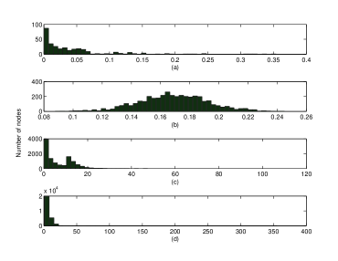
Figure 1: $50$-bin centrality histograms for a) London tube network (betweenness centrality), b) AGR network (closeness centrality), c) Gnutella-04 network (degree), and d) Gnutella-24 network (degree).

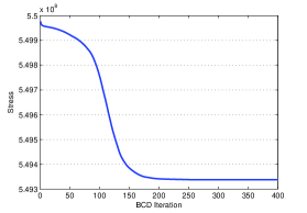
Figure 2: MDS stress vs. iterations.

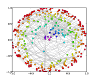
(a) $\lambda=0$

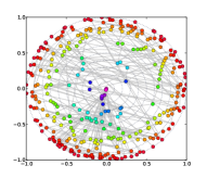
(b) $\lambda=1$

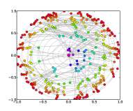
(c) $\lambda=100$

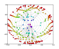
(d) $\lambda=10,000$

Figure 3: Effect of a smoothness penalty: varying $\lambda$ for the London tube visualization.

Algorithm	Betweenness centrality	Closeness centrality	Degree centrality
CC-MDS
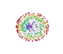
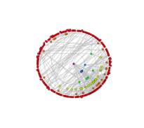
CC-LLE
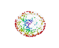
MFL
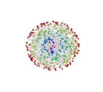
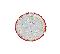
SE

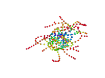
Figure 4: Embedding of the London tube graph emphasizing different centrality considerations.

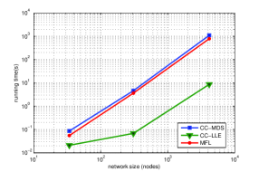
Figure 5: A comparison of running times.

9.3 Visualization of large networks

The primary focus in this subsection is large-scale network visualization and test results on three networks of varying size are considered. First among these is the ArXiv General Relativity (AGR) network, representing scientific collaborations between authors on papers submitted to the “General Relativity and Quantum Cosmology” category (January $1993$ to April $2003$) [50]. The nodes represent authors and an edge exists between nodes $i$ and $j$ if authors $i$ and $j$ co-authored a paper. Closeness centrality was used to visualize the network so that authors whose research is most related to the majority of the other authors are placed closer to the center. The distribution of closeness centrality for the AGR network is shown in Figure 1b). Node dissimilarities were based on pairwise shortest path distances between nodes.

Figure 6a) shows the embedding obtained after $30$ outer BCD iterations of running Algorithm 1. For clarity and emphasis of the node positions, edges were not included in the visualization. Drawings of graphs as large as the autonomous systems within the Internet typically thin out most of the edges. The color coding is adopted to reflect centrality variations.

CC-LLE was run for the same data yielding the network visualization depicted by Figure 6b). Only single-hop neighbors were considered ($n=1$) for the neighborhood selection. Although no claims of optimal placement or convergence are made for Algorithm 3, it is clear that the visualization succeeds at conveying the centrality structure of the collaboration network.

Next, large-scale degree visualizations of snapshots of the Gnutella peer-to-peer file-sharing network [50] were generated using CC-LLE. Nodes represent hosts and edges capture connections between them. Gnutella-$04$ and Gnutella-$24$ represent snapshots of the directed network captured in $2002$ on August $4$ and August $24$ respectively. Undirected renditions of the two networks were obtained by symmetrization of their adjacency matrices (i.e., $\mathbf{A}\leftarrow\mathbf{A}+\mathbf{A}^{\top}$). The centrality metric of interest was the node degree and dissimilarities for the two visualizations were computed based on the number of shared neighbors between any pair of hosts. Figures 6c) and 6d) depict the visualizations obtained via CC-LLE. It is clear that despite the dramatic growth of the network over a span of $20$ days, most new nodes had low degree and the number of nodes accounting for the highest degree was disproportinately small as shown in the histograms in Figures 1c) and 1d).

9.4 Running times

Running times for CC-MDS, CC-LLE and MFRL were compared for three of the networks of different dimensions. These include the karate club network ($34$ nodes), a small social network from a $1970$s study of long-term interactions between members of a U.S. university karate club. In addition, the London tube and the AGR network were considered. Figure 5 shows a log-plot of the run-times that led to embeddings with reasonably comparable visual quality. The main observation from the plot is the clear run-time advantage of CC-LLE over the other methods especially for large networks. In fact, this was the main motivation for using CC-LLE for visualizing the Gnutella networks yielding embeddings in $1,684$ s (Gnutella-$04$) and $5,639$ s (Gnutella-$24$).

10 Conclusion

In this paper, two approaches for embedding graphs with certain structural constraints were proposed. In the first approach, an optimization problem was formulated under centrality constraints that capture relative levels of importance between nodes. A block coordinate descent solver with successive approximations was developed to deal with the non-convexity and non-smoothness of the constrained MDS stress minimization problem. In addition, a smoothness penalty term was incorporated to minimize edge crossings in the resultant network visualizations. Tests on real-world networks were run and the results demonstrated that convergence is guaranteed, and large networks can be visualized relatively fast.

In the second proposed approach, LLE was adapted to the visualization problem by solving centrality-constrained optimization problems for both steps of the algorithm. The first step, which determines reconstruction weights per node, amounted to a QCQP that was solved in closed-form. The final step which determines the embedding that best preserves the weights turned out to decouple across nodes and was solved via BCD iterations with closed-form solutions per subproblem. Despite the lack of an optimality guarantee for this step, meaningful network visualizations were obtained after a few iterations making the developed algorithm attractive for large scale graph embeddings.

From an application perspective, the LLE approach is preferrable over MDS in settings where the network represents data sampled from an underlying manifold. For instance, consider a social network whose nodes represent people and edges encode self-reported friendship ties between them. It is assumed that friends have a number of similar attributes e.g., closeness in age, level of education, and income bracket. Although some of these attributes may be unknown, it is reasonable to assume that they lie near a low-dimensional nonlinear manifold, nicely motivating an LLE approach to graph embedding. Some real-world networks are heterogeneous with multi-typed nodes and edges e.g., a bibliographic network that captures the relationships between authors, conferences and papers. The manifold assumption does not apply here, but dissimilarity measures between multi-typed nodes have been developed [51], and an MDS approach is well justified.

In this work, it has been assumed that networks are static and their topologies are completely known. However, real-networks are dynamic and embeddings must be determined from incomplete data due to sampling and future research directions will incorporate these considerations.

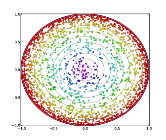
(a)

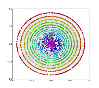
(b)

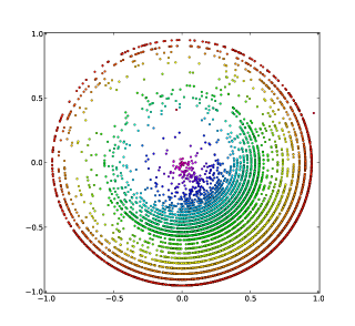
(c)

(d)

Figure 6: Visualization of large networks: a) AGR (CC-MDS), b) AGR (CC-LLE), c) Gnutella-04 (CC-LLE), and d) Gnutella-24 (CC-LLE).

Appendix A Proof of Proposition 1

Substituting ${\mathbf{x}}_{0}={\mathbf{x}}^{r-1}$ in the LHS of (12a) yields

$$\Phi({\mathbf{x}}^{r-1},{\mathbf{x}}^{r-1}) = \psi_{1}({\mathbf{x}}^{r-1})-\psi_{2}^{\prime}({\mathbf{x}}^{r-1},{\mathbf{x}}^{r-1})$$ (43)

$$= \frac{(N-1)}{2}\|{\mathbf{x}}^{r-1}\|_{2}^{2}$$

$$-({\mathbf{x}}^{r-1})^{T}(\sum_{j<i}{\mathbf{x}}_{j}^{r}+\sum_{j>i}{\mathbf{x}}_{j}^{r-1})$$

$$-\sum_{j<i}\delta_{ij}\|{\mathbf{x}}^{r-1}-{\mathbf{x}}_{j}^{r}\|_{2}$$

$$-\sum_{j>i}\delta_{ij}\|{\mathbf{x}}^{r-1}-{\mathbf{x}}_{j}^{r-1}\|_{2}.$$

Since

$$\Psi({\mathbf{x}}^{r-1}) = \psi_{1}({\mathbf{x}}^{r-1})-\psi_{2}({\mathbf{x}}^{r-1})$$ (44)

$$= \frac{(N-1)}{2}\|{\mathbf{x}}^{r-1}\|_{2}^{2}$$

$$-({\mathbf{x}}^{r-1})^{T}(\sum_{j<i}{\mathbf{x}}_{j}^{r}+\sum_{j>i}{\mathbf{x}}_{j}^{r-1})$$

$$-\sum_{j<i}\delta_{ij}\|{\mathbf{x}}^{r-1}-{\mathbf{x}}_{j}^{r}\|_{2}$$

$$-\sum_{j>i}\delta_{ij}\|{\mathbf{x}}^{r-1}-{\mathbf{x}}_{j}^{r-1}\|_{2},$$

condition (12a) is satisfied by the equivalence of (43) and (44). The second condition, (12b), is automatically satisfied for ${\mathbf{x}}_{0}={\mathbf{x}}^{r-1}$ by (7).

Appendix B Solving the KKT conditions

This appendix derives (28a) - (28e) from the KKT conditions in (29) - (31). From (28e), one obtains

$$2{\mathbf{H}}_{i}{\mathbf{w}}_{i}^{*}-2{\mathbf{h}}_{i}+2\gamma^{*}{\mathbf{H}}_{i}{\mathbf{w}}_{i}^{*}+\mu^{*}{\mathbf{1}}=\mathbf{0}.$$ (45)

Solving for ${\mathbf{w}}_{i}^{*}$ in terms of $\gamma^{*}$ and $\mu^{*}$ from (45)

$${\mathbf{w}}_{i}^{*}=\frac{1}{(1+\gamma^{*})}{\mathbf{H}}_{i}^{-1}\left({\mathbf{h}}_{i}-\frac{\mu^{*}}{2}{\mathbf{1}}\right).$$ (46)

Upon applying the result in (46) to the primal feasibility condition in (28b), it turns out that

$${\mathbf{1}}^{T}\left[\frac{{\mathbf{H}}_{i}^{-1}}{(1+\mu^{*})}\left({\mathbf{h}}_{i}-\frac{\mu^{*}}{2}{\mathbf{1}}\right)\right]=1.$$ (47)

Thus,

$$\gamma^{*}={\mathbf{1}}^{T}{\mathbf{H}}_{i}^{-1}{\mathbf{h}}_{i}-\frac{\mu^{*}}{2}{\mathbf{1}}^{T}{\mathbf{H}}_{i}^{-1}{\mathbf{1}}-1.$$ (48)

Assuming the inequality constraint is inactive at optimality, then $\gamma^{*}=0$, which upon solving (48) yields

$$\mu^{*}=\frac{2\left({\mathbf{1}}^{T}{\mathbf{H}}_{i}^{-1}{\mathbf{h}}_{i}-1\right)}{{\mathbf{1}}^{T}{\mathbf{H}}_{i}^{-1}{\mathbf{1}}}.$$ (49)

Combining (49) and (46) gives

$${\mathbf{w}}_{i}^{*}={\mathbf{H}}_{i}^{-1}\left[{\mathbf{h}}_{i}-\frac{{\mathbf{1}}^{T}{\mathbf{H}}_{i}^{-1}{\mathbf{h}}_{i}-1}{{\mathbf{1}}^{T}{\mathbf{H}}_{i}^{-1}{\mathbf{1}}}{\mathbf{1}}\right].$$ (50)

If the inequality constraint is active at optimality, then

$${\mathbf{w}}_{i}^{*T}{\mathbf{H}}_{i}{\mathbf{w}}_{i}^{*}=f^{2}(c_{i}).$$ (51)

Substituting for ${\mathbf{w}}_{i}^{*}$ from (46) results in

$$\left(2{\mathbf{h}}_{i}-\mu^{*}{\mathbf{1}}\right)^{T}{\mathbf{H}}_{i}^{-1}\left(2{\mathbf{h}}_{i}-\mu^{*}{\mathbf{1}}\right)=4f^{2}(c_{i})(1+\gamma^{*})^{2}$$ (52)

which upon simplification yields

$${\mathbf{h}}_{i}^{T}{\mathbf{H}}_{i}^{-1}{\mathbf{h}}_{i}-\mu^{*}{\mathbf{1}}^{T}{\mathbf{H}}_{i}^{-1}{\mathbf{h}}_{i}+\frac{\mu^{*2}}{4}{\mathbf{1}}^{T}{\mathbf{H}}_{i}^{-1}{\mathbf{1}}$$

$$=f^{2}(c_{i})(1+\gamma^{*})^{2}.$$ (53)

Substituting for $\gamma^{*}$ results in the following quadratic equation in $\mu^{*}$

$${\mathbf{h}}_{i}^{T}{\mathbf{H}}_{i}^{-1}{\mathbf{h}}_{i}-\mu^{*}{\mathbf{1}}^{T}{\mathbf{H}}_{i}^{-1}{\mathbf{h}}_{i}+\frac{\mu^{*2}}{4}{\mathbf{1}}^{T}{\mathbf{H}}_{i}^{-1}{\mathbf{1}}$$

$$=f^{2}(c_{i})\left({\mathbf{1}}^{T}{\mathbf{H}}_{i}^{-1}{\mathbf{h}}_{i}-\frac{\mu^{*}}{2}{\mathbf{1}}^{T}{\mathbf{H}}_{i}^{-1}{\mathbf{1}}\right)^{2}.$$ (54)

Finally, solving for $\mu^{*}$ from (B) and taking one root yields

$$\mu^{*}=2\frac{{\mathbf{1}}^{T}{\mathbf{H}}_{i}^{-1}{\mathbf{h}}_{i}}{{\mathbf{1}}^{T}{\mathbf{H}}_{i}^{-1}{\mathbf{1}}}$$

$$+2\left\{\frac{{\mathbf{h}}_{i}^{T}{\mathbf{H}}_{i}^{-1}({\mathbf{1}}{\mathbf{1}}^{T}{\mathbf{H}}_{i}^{-1}{\mathbf{h}}_{i}-{\mathbf{h}}_{i}{\mathbf{1}}^{T}{\mathbf{H}}_{i}^{-1}{\mathbf{1}})}{({\mathbf{1}}^{T}{\mathbf{H}}_{i}^{-1}{\mathbf{1}})^{2}-({\mathbf{1}}^{T}{\mathbf{H}}_{i}^{-1}{\mathbf{1}})^{3}f^{2}(c_{i})}\right\}^{\frac{1}{2}}.$$ (55)

References

- [1] E. D. Kolaczyk, Statistical Analysis of Network Data: Methods and Models, Springer, New York, NY, USA, 2009.
- [2] M. E. J. Newman, “The structure and function of complex networks,” SIAM review, vol. 45, pp. 167–256, June 2003.
- [3] B. Luo, R. C. Wilson, and E. R. Hancock, “Spectral embedding of graphs,” Pattern Recognition, vol. 36, pp. 2213–2230, January 2003.
- [4] B. Shaw and T. Jebara, “Structure preserving embedding,” International Conference of Machine Learning, Montreal, Canada, June 2009.
- [5] C. D. Correa, T. Crnovrsanin, and K.-L. Ma, ”Visual reasoning about social networks using centrality sensitivity,” IEEE Transactions on Visualization and Computer Graphics, vol. 18, pp. 106–120, January 2012.
- [6] U. Dogrusoz, M. E. Belviranli, and A. Dilek, ”CiSE: A circular spring embedder layout algorithm,” IEEE Transactions on Visualization and Computer Graphics, vol. 19, pp. 953–966, June 2013.
- [7] J. Yang, Y. Liu, X. Zhang, X. Yuan, Y. Zhao, S. Barlowe, and S. Liu, ”PIWI: Visually exploring graphs based on their community structure,” IEEE Transactions on Visualization and Computer Graphics, vol. 19, pp. 1034–1047, June 2013.
- [8] J. Abello, F. V. Ham, and N. Krishnan, ”ASK-GraphView : A large scale graph visualization system,” IEEE Transactions on Visualization and Computer Graphics, vol. 12, pp. 669–676, September 2006.
- [9] M. Girvan and M. E.J. Newman, ”Community structure in social and biological networks,” Proc. of the National Academy of Sciences U.S.A., vol. 99, pp. 7821–7826, April 2002.
- [10] Y. Jia, J. Hoberock, M. Garland, and J. Hart, ”On the visualization of social and other scale-free networks,” IEEE Transactions on Visualization and Computer Graphics, vol. 14, pp. 1285–1292, October 2008.
- [11] F. V. Ham and M. Wattenberg, ”Centrality based visualization of small world graphs,” Computer Graphics Forum, vol. 27, pp. 975–982, May 2008.
- [12] E. Giacomo, W. Didimo, L. Grilli, and G. Liotta, ”Graph visualization techniques for web clustering engines,” IEEE Transactions on Visualization and Computer Graphics, vol. 13, pp. 294–304, March 2007.
- [13] L. Harrison and A. Lu, “The future of security visualization: Lessons from network visualization,” IEEE Network, vol. 26, pp. 6–11, December 2012.
- [14] J. Ignatowicz, “Drawing force-directed graphs using optigraph,” Proceedings of DIMACS International Workshop, vol. 894, pp. 333–336, October 1994.
- [15] A. Papakostas and I. Tollis, “Algorithms for area-efficient orthogonal drawings,” Computational Geometry: Theory and Applications, vol. 9, pp. 83–110, January 1998.
- [16] E. Reingold and J. Tilford, “Tidier drawing of trees,” IEEE Trans. on Software Engineering, vol. 7, pp. 223–228, March 1981.
- [17] K. Supowit and E. Reingold, “The complexity of drawing trees nicely,” Acta Informatica, vol. 18, pp. 359–368, January 1983.
- [18] C. Wetherell and A. Shannon, “Tidy drawing of trees,” IEEE Trans. on Software Engineering, vol. 5, pp. 514–520, September 1979.
- [19] T. Biedl and G. Kant, “A better heuristic for orthogonal graph drawings,” Proceedings of the Second Annual European Symposium on Algorithms, vol. 855, pp. 24–35, September 1994.
- [20] D. Tunkelang, “A numerical optimization approach to general graph drawing,” PhD Thesis, Carnegie Mellon University School of Computer Science, January 1999.
- [21] T. Fruchterman, and E. Reingold, ”Graph drawing by force-directed placement,” Software – Practice and Experience, vol. 21, pp. 1129–-1164, November 1991.
- [22] G. Sabidussi, “The centrality index of a graph,” Psychometrika, vol. 31, pp. 581–-683, December 1966.
- [23] L. C. Freeman, “A set of measures of centrality based on betweenness,” Sociometry, vol. 40, pp. 35–41, March 1977.
- [24] P. Jaccard, “Étude comparative de la distribution florale dans une portion des Alpes et des Jura,” Bulletin de la Societé Vaudoise des Sceience Naturelles, vol. 37, pp. 547–579, November 1901.
- [25] E. Ravasz, A. L. Somera, D. A. Mongru, Z. N. Oltvai, A. L. Barabási, “Hierarchical organization of modularity in metabolic networks”, Science, vol. 297, pp. 1551–1555, August 2002.
- [26] E. A. Leicht, P. Holme, M. E. J. Newman, “Vertex similarity in networks”, Physical Review E, vol. 73, 026120, February 2006.
- [27] D. J. Klein, M. Randic, “Resistance distance”, Journal of Mathematical Chemistry, vol. 12, pp. 81–95, December 1993.
- [28] L. Page, S. Brin, R. Motwani, and T. Winograd, “The PageRank citation ranking: bringing order to the web.”, Stanford InfoLab, November 1999.
- [29] W. Liu, L. Lü, Jin, T. Zhou, “Link prediction based on local random walk,” Europhysics Letters, vol. 89, 58007, March 2010.
- [30] U. Brandes and C. Pich, “More flexible radial layout,” Journal of Graph Algorithms and Applications, vol. 15, pp. 157–173, February 2011.
- [31] I. Borg and P. J. Groenen, Modern Multidimensional Scaling: Theory and Applications, Springer, New York, NY, 2005.
- [32] M. Belkin and P. Niyogi, “Laplacian eigenmaps for dimensionality reduction and data representation,” em Neural computation, vol. 15, pp. 1373–1396, June 2003.
- [33] T. Kamada and S. Kawai, “An algorithm for drawing general undirected graphs,” Information Processing Letters, vol. 31, pp. 7–15, April 1989.
- [34] L. K. Saul, and S. T. Roweis, “Think globally, fit locally: unsupervised learning of low dimensional manifolds,” Journal of Machine Learning Research, vol. 4, pp. 119–155, June 2003.
- [35] J. B. Tenenbaum, V. de Silva, and J. C. Langford, “A global geometric framework for nonlinear dimensionality reduction,” Science, vol. 290, pp. 2319–2323, December 2000.
- [36] D. De Ridder, O. Kouropteva, O. Okun, M. Pietikainen, and R. Duin, “Supervised locally linear embedding,” Artificial Neural Networks and Neural Information Processing-ICANN/ICONIP, pp. 175–175, June 2003.
- [37] H. Chang and Y. Dit-Yan, “Robust locally linear embedding,” Pattern Recognition, vol. 39, pp. 1053–1065, June 2006.
- [38] T. Hastie, R. Tibshirani, and J. Friedman, The Elements of Statistical Learning: Data Mining, Inference, and Prediction, Springer, New York, NY, USA, 2001.
- [39] J. Alvarez-Hamelin, L. Dall’Asta, A. Barrat, and A. Vespignani, “Large scale networks fingerprinting and visualization using the k-core decomposition,” Advances in Neural Information Processing Systems, vol. 18, pp. 41–50, May 2006.
- [40] F. Fouss, A. Pirotte, J. M. Renders, and M. Saerens, “Random-walk computation of similarities between nodes of a graph with application to collaborative recommendation,” IEEE Transactions on Knowledge and Data Engineering, vol. 19, pp. 355–369, March 2007.
- [41] S. L. France and J. D. Carroll, “Two-way multidimensional scaling: a review,” IEEE Transactions on Systems, Man, and Cybernetics, vol. 41, pp. 644–661, September 2011.
- [42] K. Q. Weinberger and L. K. Saul, “Unsupervised learning of image manifolds by semidefinite programming,” Proceedings of the IEEE Computer Society Conference on Computer Vision and Pattern Recognition, vol. 2, pp. 988–995, July 2004.
- [43] K. Q. Weinberger, B. D. Packer, and L. K. Saul, “Nonlinear dimensionality reduction by semidefinite programming and kernel matrix factorization,” Proceedings of the 10th International Workshop on Artificial Intelligence and Statistics, pp. 381–388, January 2005.
- [44] S. Boyd and L. Vandenberghe, Convex Optimization, Cambridge University Press, New York, NY, 2004.
- [45] D. P. Bertsekas, Nonlinear programming, Athena Scientific, Belmont, MA, 1999.
- [46] M. Razaviyayn, M. Hong, and Z. Q. Luo, “A unified convergence analysis of block successive minimization methods for nonsmooth optimization,” arXiv preprint arXiv:1209.2385v1, September 2012.
- [47] B. Baingana, and G. B. Giannakis, “Centrality-constrained graph embedding,” Proc. of the 38th Intern. Conf. on Acoust., Speech and Signal Proc., Vancouver, Canada, May 26–31, 2013.
- [48] K. Q. Weinberger, F. Sha, Q. Zhu, and L. K. Saul, “Graph Laplacian regularization for large-scale semidefinite programming,” Advances in Neural Information Processing Systems, vol. 19, pp. 1489–1496, September 2007.
- [49] A. Buja, D. F. Swayne, M. L. Littman, N. Dean, H. Hofmann, and L. Chen, “Data visualization with multidimensional scaling,” Journal of Comp. and Graph. Stats., pp. 444–472, June 2008.
- [50] J. Leskovec, J. Kleinberg, and C. Faloutsos, “Graph evolution: Densification and shrinking diameters,” ACM Transactions on Knowledge Discovery from Data, vol. 1, article 2, March 2007.
- [51] C. Shi, X. Kong, P. S. Yu, S. Xie, and B. Wu, “Relevance search in heterogeneous networks,” Proceedings of the 15th International Conf. on Extending Database Technology, pp. 180–191, March 2012.