The ³He$(e,e^{\prime}p)^{2}$H and ⁴He$(e,e^{\prime}p)^{3}$H reactions at high momentum transfer

Abstract

We present updated calculations for observables in the processes ³He($e,e^{\prime}p$)²H, ⁴He($e,e^{\prime}p$)³H, and ⁴He($\vec{e},e^{\prime}\vec{p}\,$)³H. This update entails the implementation of improved nucleon-nucleon ($NN$) amplitudes to describe final state interactions (FSI) within a Glauber approximation and includes full spin-isospin dependence in the profile operator. In addition, an optical potential, which has also been updated since previous work, is utilized to treat FSI for the ⁴He($e,e^{\prime}p$)³H and ⁴He($\vec{e},e^{\prime}\vec{p}\,$)³H reactions. The calculations are compared with experimental data and show good agreement between theory and experiment. Comparisons are made between the various approximations in the Glauber treatment, including model dependence due to the $NN$ scattering amplitudes, rescattering contributions, and spin dependence. We also analyze the validity of the Glauber approximation at the kinematics the data is available, by comparing to the results obtained with the optical potential.

I Introduction

Recent experiments at Jefferson Lab (JLab) have measured cross sections and polarization observables for the ³He($e,e^{\prime}p$)²H, ⁴He($e,e^{\prime}p$)³H, and ⁴He($\vec{e},e^{\prime}\vec{p}\,$)³H reactions at intermediate and large momentum transfers Rvachev et al. (2005); Reitz (2004); Strauch et al. (2003); Paolone et al. (2010); Malace et al. (2011) . These data have generated considerable interest in the nuclear few-body community, as attested by the series of papers dealing with the description of the proton-knockout mechanism and the treatment of final state interactions (FSI) at GeV energies, which have appeared in the literature in last few years  degli Atti and Kaptari (2005); Ciofi degli Atti and Kaptari (2005); degli Atti and Kaptari (2008); Alvioli et al. (2010); Laget (2005a, b); Sargsian et al. (2005a, b).

In the present work, we report on a calculation of the two-body electrodisintegration cross sections of ³He and ⁴He in the wide range of momentum transfers covered by the JLab experiments. This study updates, improves, and extends that of Refs. Schiavilla et al. (2005a, b). As in the earlier work, the nuclear bound states are represented by non-relativistic wave functions, obtained from realistic two- and three-nucleon potentials (the Argonne $v_{18}$ two-nucleon Wiringa et al. (1995) and Urbana IX three-nucleon Pudliner et al. (1995) potentials—the AV18/UIX Hamiltonian) and FSI between the outgoing proton and recoiling bound cluster are treated either in the Glauber approximation for the $A$=3 and 4 reactions—with inclusion in the associated profile operator of the full spin-isospin dependence of the nucleon-nucleon ($NN$) elastic scattering amplitude—or, in the case of the $A$=4 reactions, with an optical potential. Important differences between the present work and that of Refs. Schiavilla et al. (2005a, b) are that: i) the $NN$ amplitudes are obtained from the Scattering Analysis Interactive Dial-in (SAID) analysis Arndt et al. (2000, 2007); SAI of $pn$ ($pp$) scattering data at lab kinetic energies ranging from 0.05 (0.05) GeV to 1.3 (3.0) GeV rather than from a parametrization of these amplitudes valid at forward scattering (at small momentum transfers) Wallace (1981), and ii) the parameters in the optical potential have been adjusted to reproduce, in addition to ³H($p,p$)³H elastic and ³H($p,n$)³He charge-exchange cross section data, also the induced polarization data recently measured for the ⁴He($\vec{e},e^{\prime}\vec{p}\,$)³H reaction at JLab Malace et al. (2011).

This paper is organized as follows. In Sec. II, we briefly discuss our treatment of FSI both in the Glauber and optical-model approximations, relegating details on the construction of the Glauber profile operator from the $NN$ SAID amplitudes to Appendices A and B. In Sec. III we review the bound-state wave functions, the model for the electromagnetic current operator, and the Monte Carlo methods used in the numerical evaluation of the relevant matrix elements—these methods have already been described in considerable detail in Ref. Schiavilla et al. (2005a). In Sec IV we list explicit expressions for the observables of interest to this work. Finally, in Sec. V we present a detailed discussion of the results, including a comparison between the Glauber and optical-model treatment of FSI in kinematical regimes where both approaches are expected to be valid, and in Sec. VI we summarize our conclusions.

II Final state interactions

Two different approximations are adopted in the present work to describe FSI in the two-body electrodisintegrations of ³He and ⁴He: one is based on the Glauber approach Glauber (1959), while the other, whose application is limited only to processes involving ⁴He, relies on an optical potential. Both approximations have been discussed in considerable detail in Refs. Schiavilla et al. (2005a) and Schiavilla et al. (2005b): each has limitations as to the energy range where it is expected to be reliable. For completeness, in this section we briefly review them, emphasizing those aspects of the approach which have been improved since the study of Refs. Schiavilla et al. (2005a, b).

II.1 Glauber approach

In this approach the wave function of the final $p$+($A-1$) system is written as

$$\psi(p+^{(A-1)}\!f;{\rm GLB})=\frac{1}{\sqrt{A}}\sum_{\cal P}\epsilon_{\cal P}\,G(A;1\dots A-1)\,{\rm e}^{{\rm i}{\bf p}\cdot{\bf r}_{A}}\chi_{\sigma}(A;p)\,{\rm e}^{{\rm i}{\bf p}_{f}\cdot{\bf R}_{1\dots A-1}}\phi_{\sigma_{f}}(1\dots A-1;f)\ ,$$ (1)

where $\chi_{\sigma}(p)$ represents a proton in spin state $\sigma$, $\phi_{\sigma_{f}}(f)$ denotes the wave function of the ($A-1$)-system with spin projection $\sigma_{f}$, and ${\bf R}_{1\dots A-1}$ is the center-of-mass position vector of the $A-1$ nucleons in this cluster. The sum over permutations $\cal P$ of parity $\epsilon_{\cal P}$ ensures the overall antisymmetry of $\psi(p+^{(A-1)}\!f;{\rm GLB})$.

The operator $G(A;1\dots A-1)$ inducing FSI can be derived from an analysis of the multiple scattering series by requiring that the struck (fast) nucleon (nucleon $A$) is undeflected by rescattering processes, and that the nucleons in the residual system (nucleons $1,\dots,A-1$) act as fixed scattering centers Wallace (1981). It is expanded as

$$G=1+\sum_{n=1}^{A-1}(-)^{n}G^{(n)}\ ,$$ (2)

where $G^{(n)}$ represents the $n^{\rm th}$ rescattering term, and therefore for an $A$-body system up to $A-1$ rescattering terms are generally present. The leading single-rescattering term reads

$$G^{(1)}(A;1\dots A-1)=\sum_{i=1}^{A-1}\theta(z_{iA})\,\Gamma_{iA}({\bf b}_{iA};s_{iA})\ ,$$ (3)

where $z_{iA}$ and ${\bf b}_{iA}$ denote the longitudinal and transverse components of ${\bf r}_{i}-{\bf r}_{A}$ relative to $\hat{\bf p}$, the direction of the nucleon momentum,

$$z_{iA}\equiv{\hat{\bf p}}\cdot({\bf r}_{i}-{\bf r}_{A})\ ,\qquad{\bf r}_{i}-{\bf r}_{A}\equiv{\bf b}_{iA}+z_{iA}\,{\hat{\bf p}}\ ,$$ (4)

and the step-function $\theta(x)$, $\theta(x)=1$ if $x>0$ and $\theta(x)=0$ if $x<0$, prevents the occurrence of backward scattering for the struck nucleon. The “profile operator”$\ \Gamma_{iA}$, derived from the $N$$N$ elastic scattering amplitude at the invariant energy $\sqrt{s_{iA}}$, is discussed below. The double- and triple-rescattering terms, relevant for the present study of the ³He($e,e^{\prime}p$)$d$ and ⁴He($e,e^{\prime}p$)$t$ reactions, are given by

$$G^{(2)}(A;1\dots A-1)=\sum_{i\neq j=1}^{A-1}\theta(z_{ij})\,\theta(z_{jA})\,\Gamma_{iA}({\bf b}_{iA};s_{iA})\,\Gamma_{jA}({\bf b}_{jA};s_{jA})\ ,$$ (5)

$$G^{(3)}(A;1\dots A-1)=\sum_{i\neq j\neq k=1}^{A-1}\theta(z_{ij})\,\theta(z_{jk})\,\theta(z_{kA})\,\Gamma_{iA}({\bf b}_{iA};s_{iA})\,\Gamma_{jA}({\bf b}_{jA};s_{jA})\,\Gamma_{kA}({\bf b}_{kA};s_{kA})\ ,$$ (6)

where the product of $\theta$-functions ensures the correct sequence of rescattering processes in the forward hemisphere.

The profile operator $\Gamma_{ij}$ is related to the $N$$N$ scattering amplitude, denoted as $F_{ij}({\bf k};s)$, via the Fourier transform

$$\Gamma_{ij}({\bf b};s)=\frac{1}{2\pi{\rm i}\,p}\int{\rm d}^{2}{\bf k}\,{\rm e}^{-{\rm i}{\bf k}\cdot{\bf b}}F_{ij}({\bf k};s)\ ,$$ (7)

where, in the eikonal limit, the momentum transfer ${\bf k}$ is perpendicular to ${\bf p}$. The isospin symmetry of the strong interactions allows one to express $F_{ij}$ as

$$F_{ij}=F_{ij,+}+F_{ij,-}{\bm{\tau}}_{i}\cdot{\bm{\tau}}_{j}\ ,$$ (8)

where the $F_{ij,\pm}$ are related to the physical amplitudes for $p$$p$ and $p$$n$ scattering (see below). The invariant energy $\sqrt{s_{iA}}$ is determined as follows Schiavilla et al. (2005a). Nucleon $A$ denotes the knocked-out nucleon with momentum ${\bf p}_{A}$=${\bf p}$ and energy $E_{A}$=$E$ (${\bf p}$ and $E$ are the momentum and energy of the outgoing proton in the lab frame), while nucleons $1,\dots,A-1$, making up the bound cluster ($d$ or $t$), have momenta ${\bf p}_{1},\dots,{\bf p}_{A-1}$, with ${\bf p}_{1}+\dots+{\bf p}_{A-1}$=${\bf p}_{f}$ (${\bf p}_{f}$ is the momentum of the recoiling cluster in the lab frame). The invariant energy $\sqrt{s_{iA}}$, $i$=$1,\dots,A-1$, is obtained from

$$s_{iA} = (E_{i}+E_{A})^{2}-({\bf p}_{i}+{\bf p}_{A})^{2}$$ (9)

$$\simeq 2\,m^{2}+2\,E\,\sqrt{{\bf p}_{f}^{2}/(A-1)^{2}+m^{2}}-2\,{\bf p}\cdot{\bf p}_{f}/(A-1)\ ,$$

where in the second line the nucleons $1,\dots,A-1$ in the recoiling cluster are assumed to share its momentum equally, ${\bf p}_{i}\simeq{\bf p}_{f}/(A-1)$. The momenta of nucleon $A$ and nucleon $i$, $i$=$1,\dots,A-1$, after rescattering are ${\bf p}-{\bf k}$ and ${\bf p}_{f}/(A-1)+{\bf k}$. The $A-2$ spectator nucleons ($j\neq i$) have each momentum ${\bf p}_{f}/(A-1)$. The pair $iA$ “rescattering frame”we refer to in the following is defined as that in which nucleon $A$ and nucleon $i$ have initial momenta ${\bf p}$ and ${\bf p}_{f}/(A-1)$ and final momenta ${\bf p}-{\bf k}$ and ${\bf p}_{f}/(A-1)+{\bf k}$, respectively.

We adopt the notation of Ref. Schiavilla et al. (2005a) and parameterize the $N$$N$ scattering amplitude in the c.m. frame as

$$(2{\rm i}\,\overline{p})^{-1}\,\overline{F}^{\,NN}_{ij}(\,\overline{{\bf k}},s)=\sum_{m=1}^{5}\overline{F}^{\,NN}_{m}(\overline{{\bf k}}^{\,2}\!,s)\overline{O}^{\,m}_{ij}\ ,$$ (10)

where $\overline{\bf p}$ and $\overline{\bf p}^{\,\prime}$ denote the initial and final nucleon momenta, respectively, the $\overline{F}^{\,NN}_{m}$’s are functions of the invariant energy $\sqrt{s}$ and momentum transfer $\overline{\bf k}^{\,2}$ (with $\overline{\bf k}=\overline{\bf p}-\overline{\bf p}^{\,\prime}$), and the five operators $\overline{O}^{\,m}_{ij}$, including central, single and double spin-flip terms, are those listed in Eq. (3.11) of Ref. Schiavilla et al. (2005a). The overline is to indicate that the quantities above are in the c.m. frame.

In Ref. Schiavilla et al. (2005a) we used for the functions $\overline{F}^{\,NN}_{m}$ the Gaussian parameterizations obtained by Wallace in 1981 Wallace (1981). In the present work, instead, we derive them from the SAID analysis Arndt et al. (2000, 2007); SAI of $N$$N$ elastic scattering data from threshold up to lab kinetic energies of 3 GeV ($pp$) and 1.3 GeV ($pn$). In Appendix A we discuss how the Wallace form of the amplitudes is obtained from the SAID helicity amplitudes.

Once the amplitude in Eq. (10) has been determined in the c.m. frame, it is necessary to boost it to the rescattering frame. This is carried out with the procedure described in Refs. Schiavilla et al. (2005a); McNeil et al. (1983a), which consists of two steps. First, we introduce an invariant representation of the amplitude,

$${\cal F}^{NN}_{ij}=\sum_{m=1}^{5}{\cal F}_{m}^{NN}(s,t)\Lambda_{ij}^{m}\ ,$$ (11)

where the five operators $\Lambda_{ij}^{m=1,\dots,5}$ are $1\,,\,\gamma_{i}^{\mu}\,\gamma_{j,\mu}\,,\,\sigma_{i}^{\mu\nu}\,\sigma_{j,\mu\nu}\,,\,\gamma_{i}^{5}\,\gamma_{j}^{5}\,,\,\gamma^{5}_{i}\,\gamma_{i}^{\mu}\,\gamma^{5}_{j}\,\gamma_{j,\mu}\ ,$ and determine the invariant functions ${\cal F}_{m}^{NN}(s,t)$ from the $\overline{F}^{\,NN}_{m}$’s in the c.m. frame as in Ref. Schiavilla et al. (2005a)—however, the momentum transfer dependence of the matrix $\overline{M}_{mn}(\overline{p},\overline{\bf k}^{\,2})$ in Eq. (3.16) of Ref. Schiavilla et al. (2005a), which was neglected in that work, is now fully retained.

Next, the scattering amplitude in the rescattering frame is obtained from

$$\chi_{\sigma_{i}^{\prime}}^{\dagger}\chi_{\sigma_{j}^{\prime}}^{\dagger}\left[(2{\rm i}\,p)^{-1}\,F^{NN}_{ij}({\bf k},s)\right]\chi_{\sigma_{i}}\chi_{\sigma_{j}}=\overline{u}_{\sigma_{i}^{\prime}}({\bf p}-{\bf k})\overline{u}_{\sigma_{j}^{\prime}}({\bf p}_{f}/(A-1)+{\bf k}){\cal F}^{NN}_{ij}u_{\sigma_{i}}({\bf p})u_{\sigma_{j}}({\bf p}_{f}/(A-1))\ ,$$ (12)

where the $u_{\sigma}$ are (positive-energy) Dirac spinors with $\overline{u}_{\sigma}\equiv u_{\sigma}^{\dagger}\gamma^{0}$, and $\chi_{\sigma}$ are two-component Pauli spinors. In practice, the dependence upon ${\bf p}_{f}/(A-1)$ in the spinors of particle $j$ is neglected (in this limit, the rescattering and lab frames for the interacting $N$$N$ pair coincide). This is justified as long as $p_{f}/(A-1)$ is not too large relative to $p$, the momentum of the fast ejected proton, a condition satisfied at low missing momenta $p_{f}$ in the experiments of Refs. Rvachev et al. (2005); Reitz (2004); Strauch et al. (2003). The resulting $F^{NN}_{ij}({\bf k},s)$ has central, single and double spin-flip terms, and is given explicitly in Appendix B.

Finally, carrying out the (two-dimensional) Fourier transform in Eq. (7) leads to the profile operator

$$\Gamma_{ij}({\bf b};s) = \Gamma^{(1)}_{ij}(b;s)+\Gamma^{(2)}_{ij}(b;s)\,{\bm{\sigma}}_{i}\cdot{\bm{\sigma}}_{j}+\left[\Gamma^{(3)}_{ij}(b;s)\,{\bm{\sigma}}_{i}+\Gamma^{(4)}_{ij}(b;s)\,{\bm{\sigma}}_{j}\right]\cdot{\bf b}\times\hat{\bf p}$$ (13)

$$+ \Gamma^{(5)}_{ij}(b;s)\,{\bm{\sigma}}_{i}\cdot{\bf b}\,\,{\bm{\sigma}}_{j}\cdot{\bf b}+\Gamma^{(6)}_{ij}(b;s)\,{\bm{\sigma}}_{i}\cdot\hat{\bf p}\,\,{\bm{\sigma}}_{j}\cdot\hat{\bf p}+\Gamma^{(7)}_{ij}(b;s)\,{\bm{\sigma}}_{i}\cdot{\bf b}\,\,{\bm{\sigma}}_{j}\cdot\hat{\bf p}$$

$$+ \Gamma^{(8)}_{ij}(b;s)\,{\bm{\sigma}}_{i}\cdot\hat{\bf p}\,\,{\bm{\sigma}}_{j}\cdot{\bf b}\ ,$$

where the isospin-dependent operators $\Gamma^{(m)}_{ij}$, $m=1,\dots,8$, are given by

$$\Gamma^{(m)}_{ij}(b;s)=\Gamma^{(m)}_{+}(b;s)+\Gamma^{(m)}_{-}(b;s)\,{\bm{\tau}}_{i}\cdot{\bm{\tau}}_{j}\ .$$ (14)

The profile functions $\Gamma^{(m)}_{\pm}$ are related to those corresponding to $p$$p$ and $p$$n$ elastic scattering, obtained in Appendix B, via

$$\Gamma^{(m)}_{\pm}=\left(\Gamma^{(m)}_{pp}\pm\Gamma^{(m)}_{pn}\right)\!/2\ .$$ (15)

II.2 Optical potential

To describe FSI effects in the ⁴He($e,e^{\prime}p$)³H and ⁴He($\vec{e},e^{\prime}\vec{p}\,$)³H reactions, we also use an optical potential Schiavilla et al. (2005b); van Oers et al. (1982); Schiavilla (1990). In this case, the $p\,^{3}$H wave function reads

$$\psi^{(-)}_{{\bf k}\sigma;\sigma_{3}}(p+^{3}\!{\rm H};{\rm OPT})=\frac{{\rm e}^{{\rm i}({\bf p}+{\bf p}_{3})\cdot{\bf R}_{1\dots 4}}}{\sqrt{4}}\sum_{\cal P}\epsilon_{\cal P}\Big{[}\eta_{{\bf k}\sigma}^{(-)}(i;p)\phi_{\sigma_{3}}(jkl;^{3}\!{\rm H})+\eta_{{\bf k}\sigma}^{(-)}(i;n)\phi_{\sigma_{3}}(jkl;^{3}\!{\rm He})\Big{]}\ ,$$ (16)

where $\sigma$ and $\sigma_{3}$ are the spectator nucleon and bound cluster spin projections, ${\bf k}$ and ${\bf p}+{\bf p}_{3}$ are their relative and total momenta, respectively.

The spectator wave functions $\eta(i;p/n)$ are obtained from the linear combinations $[\eta(i;T=1)$$+/-$$\eta(i;T=0)]/2$, where $T$=0,1 denotes the total isospin of the 1+3 clusters. The latter are taken to be the scattering solutions of a Schrödinger equation containing a complex, energy-dependent optical potential of the form

$$v^{\rm opt}_{T}(T_{\rm rel})=[v^{c}(r;T_{\rm rel})+(4T-3)v^{c\tau}(r;T_{\rm rel})]+[v^{b}(r;T_{\rm rel})+(4T-3)v^{b\tau}(r;T_{\rm rel})]\,{\bf l}\cdot{\bf s}\ ,$$ (17)

where $T_{\rm rel}$ is the relative energy between clusters $i$ and $j$$k$$l$, and ${\bf l}$ and ${\bf s}$ are the orbital and spin angular momenta of nucleon $i$, respectively. The imaginary part of $v^{\rm opt}_{T}$ accounts for the loss of flux in the $p\,^{3}$H and $n\,^{3}$He states due to their coupling to the $dd$, three- and four-body breakup channels of ⁴He. Note that the $n$+³He component in the scattering wave function $\psi^{(-)}(p+^{3}\!{\rm H})$ vanishes unless the isospin-dependent (charge-exchange) terms in $v^{\rm opt}$ are included. In the results presented in Sec. V, all partial waves are retained in the expansion of $\eta(i;T)$, with full account of interaction effects in those with relative orbital angular momentum $l\leq 17$. It has been explicitly verified that the numerical importance of FSI in higher partial waves is negligible.

The central $v^{c}$ and $v^{c\tau}$, and spin-orbit $v^{b}$ and $v^{b\tau}$ terms have standard Woods-Saxon and Thomas functional forms. The parameters of $v^{c}$ and $v^{b}$ were determined by fitting $p+^{3}{\rm H}$ elastic cross section data in the lab energy range $T_{\rm lab}$=(160–600) MeV, see Ref. van Oers et al. (1982) for a listing of their values. The parameters of the $v^{c\tau}$ and $v^{b\tau}$ terms have been constrained by fitting $p+^{3}{\rm H}\rightarrow n+^{3}{\rm He}$ charge-exchange cross section data at $T_{\rm lab}$=57 MeV and 156 MeV Schiavilla (1990) and the induced polarization $P_{y}$ measured in the ⁴He($e,e^{\prime}\vec{p}\,)^{3}$H reaction Malace et al. (2011). The charge-exchange central term has a real part given by $[7.60-0.033\,T_{\rm lab}({\rm MeV})]$ MeV with radius and diffuseness of 1.2 fm and 0.15 fm and an imaginary part given by $[0.893-0.0025\,T_{\rm lab}({\rm MeV})]$ MeV with radius and diffuseness of 1.8 fm and 0.2 fm, while the charge-exchange spin-orbit term is taken to be purely real, with a depth parameter depending logarithmically on $T_{\rm lab}$, $[-15.0+1.5\,{\rm log}\,T_{\rm lab}({\rm MeV})]$ in MeV, and with radius and diffuseness having the values 1.2 fm and 0.15 fm, respectively (note that in Ref. Schiavilla et al. (2005b) the sign of the depth parameter of this term had been reported erroneously with the opposite sign).

III Calculation

In this section we give, for completeness, a brief summary of those aspects of the calculations, relating to the bound cluster wave functions, nuclear electromagnetic current, and Monte Carlo methods used in evaluating the matrix elements, which have already been reviewed in considerable detail in Refs. Schiavilla et al. (2005a, b) and references therein.

The bound states of the three- and four-nucleon systems are represented by variational wave functions, obtained with the hyperspherical-harmonics (HH) technique Viviani et al. (2005) from a realistic Hamiltonian consisting of the Argonne $v_{18}$ Wiringa et al. (1995) and Urbana-IX Pudliner et al. (1995) (AV18/UIX) potentials. These potentials and the resulting wave functions have been shown to account successfully at a quantitative level for a wide variety of three- and four-nucleon properties, such as binding energies and charge radii Viviani et al. (2005).

The nuclear electromagnetic current includes one- and two-body components. The one-body operators, listed in Ref. Schiavilla et al. (2005a), are derived from an expansion of the covariant single-nucleon current Jeschonnek and Donnelly (1998). The two-body operators used in the present work are discussed in the review paper Carlson and Schiavilla (1998) (and references therein). The leading terms are derived from the static part of the AV18 potential, which is assumed to be due to exchanges of effective pseudo-scalar ($\pi$-like) and vector ($\rho$-like) mesons. The corresponding charge and current operators are constructed from non-relativistic reductions of Feynman amplitudes with the $\pi$-like and $\rho$-like effective propagators projected out of the central, spin-spin and tensor components of the AV18. Additional (short-range) currents result from minimal substitution in its momentum-dependent components. These charge and current operators contain no free parameters, and their short-range behavior is consistent with that of the AV18. The (purely transverse) two-body currents associated with $M1$-excitation of $\Delta$ resonances in the intermediate state, and from $\rho\pi\gamma$ and $\omega\pi\gamma$ transition mechanisms are also included. As documented in Refs. Carlson and Schiavilla (1998); Carlson et al. (2002); Marcucci et al. (2005), these charge and current operators reproduce quite well a variety of few-nucleon electromagnetic observables, ranging from elastic form factors to low-energy radiative capture cross sections to the quasi-elastic response in inclusive $(e,e^{\prime})$ scattering at intermediate energies.

The Höhler parameterization Hohler et al. (1976) is used for the electromagnetic form factors of the nucleon. In the analysis of the ⁴He($\vec{e},e^{\prime}\vec{p}\,$)³H experiment, however, at the highest $Q^{2}$ values of 1.6 (GeV/c)² and 2.6 (GeV/c)² the proton electric and magnetic form factors are taken from the parameterization obtained in Ref. Brash et al. (2002) by fitting $G_{Mp}$ data and the ratio $G_{Ep}/G_{Mp}$ recently measured at JLab Jones et al. (2000).

Finally, the numerical evaluation of the relevant matrix elements is carried out by a combination of Monte Carlo methods and standard quadrature techniques, described for the case of $A$=3 in Ref. Schiavilla et al. (2005a). This hybrid approach is easily generalized to the $A$=4 case: indeed, it was already used in the calculations reported in Ref. Schiavilla et al. (2005b). The resulting predictions are numerically “exact”, apart from small statistical errors due to the Monte Carlo integration, and therefore suffer from no further approximations beyond those inherent to the treatment of FSI and nuclear electromagnetic currents.

IV Observables

For clarity we briefly recap the observables of interest for this calculation. More details can be found in Refs. Schiavilla et al. (2005a, b) for observables relevant to the ³He($e,e^{\prime}p$)²H and ⁴He($e,e^{\prime}p$)³H reactions, respectively.

The five-fold differential cross section for the ${}^{A}i(e,e^{\prime}p)^{(A-1)}f$ process is given as

$$\frac{d^{5}\sigma}{dE_{e}^{\prime}d\Omega_{e}^{\prime}d\Omega}=p\,E\,\sigma_{\rm Mott}\,f_{\rm rec}\frac{m}{E}\frac{m_{f}}{E_{f}}\left[v_{L}R_{L}+v_{T}R_{T}+v_{LT}\,R_{LT}\cos(\phi)+v_{TT}R_{TT}\cos(2\phi)\right],$$ (18)

where $E_{e}^{\prime}$ is the energy of the final electron, $\Omega_{e}^{\prime}$ and $\Omega$ are, respectively, the solid angles of the final electron and ejected proton, $m_{f}$ is the rest mass of the ($A$–1)-cluster, ${\bf p}$ and $E$ (${\bf p}_{f}$ and $E_{f}$) are the momentum and energy of the proton (($A$–1)-cluster), $\phi$ is the angle between the electron scattering plane and the plane defined by ${\bf q}$ and ${\bf p}$, and the recoil factor is defined by its inverse

$$f_{\rm rec}^{-1}=\left|1-\frac{p_{f}\,E}{p\,E_{f}}{\hat{\bf p}}\cdot{\hat{\bf p}}_{f}\right|.$$ (19)

For a derivation of Eq. (18), the definition of $\sigma_{\rm Mott}$ and of the (standard) electron kinematic factors, $v_{\alpha}$, where $\alpha=L,T,LT,TT$, see Ref. Raskin and Donnelly (1989). The nuclear response functions are given in Ref. Schiavilla et al. (2005a).

The longitudinal-transverse asymmetry $A_{LT}$ is obtained from the differential cross sections

$$A_{LT} =\frac{\sigma(\phi=0^{\circ})-\sigma(\phi=180^{\circ})}{\sigma(\phi=0^{\circ})+\sigma(\phi=180^{\circ})}$$

$$=\frac{v_{LT}R_{LT}}{v_{L}R_{L}+v_{T}R_{T}+v_{TT}R_{TT}},$$ (20)

where $\sigma(\phi)$ represents the differential cross section in Eq. (18).

In parallel kinematics, where the electron three-momentum transfer ${\bf q}$ and the missing momentum ${\bf p}_{m}$ (defined as ${\bf p}_{m}=-{\bf p}_{f}={\bf p}-{\bf q}$) are parallel, the polarization transfers $P_{x}^{\prime}$ and $P_{z}^{\prime}$ are given by

$$P_{x}^{\prime}=\frac{v_{LT^{\prime}}R^{t}_{LT^{\prime}}}{v_{L}R_{L}+v_{T}R_{T}}\ ,\qquad P_{z}^{\prime}=\frac{v_{TT^{\prime}}R^{l}_{TT^{\prime}}}{v_{L}R_{L}+v_{T}R_{T}}\ ,$$ (21)

where the response functions $R^{t}_{LT^{\prime}}$ and $R^{l}_{TT^{\prime}}$ and electron kinematical factors $v_{LT^{\prime}}$ and $v_{TT^{\prime}}$ read Picklesimer and Van Orden (1989)

$$R^{t}_{LT^{\prime}} = 2\,\sqrt{2}\sum_{m_{3}}{\rm Im}\Big{[}\langle p+^{3}\!{\rm H};+\hat{\bf x},m_{3}\!\mid\rho(q\hat{\bf z})\mid^{4}\!{\rm He}\rangle\,\langle p+^{3}\!{\rm H};+\hat{\bf x},m_{3}\!\mid j_{y}(q\hat{\bf z})\mid^{4}\!{\rm He}\rangle^{*}\Big{]}\ ,$$ (22)

$$R^{l}_{TT^{\prime}} = 2\sum_{m_{3}}{\rm Im}\Big{[}\langle p+^{3}\!{\rm H};+\hat{\bf z},m_{3}\!\mid j_{x}(q\hat{\bf z})\mid^{4}\!{\rm He}\rangle\,\langle p+^{3}\!{\rm H};+\hat{\bf z},m_{3}\!\mid j_{y}(q\hat{\bf z})\mid^{4}\!{\rm He}\rangle^{*}\Big{]}\ ,$$ (24)

$$v_{LT^{\prime}}=\frac{1}{\sqrt{2}}\,\frac{Q^{2}}{q^{2}}{\rm tan}(\theta_{e}/2)\ ,\qquad v_{TT^{\prime}}={\rm tan}(\theta_{e}/2)\sqrt{\frac{Q^{2}}{q^{2}}+{\rm tan}^{2}(\theta_{e}/2)}\ .$$

and $\theta_{e}$ and $Q^{2}=q^{2}-\omega^{2}$ are, respectively, the electron scattering angle and four-momentum transfer. In the above equations, $\mid\!^{4}{\rm He}\rangle$ represents the ⁴He ground state, while $\mid\!p+^{3}\!{\rm H};+\hat{\bf x},m_{3}\rangle$ and $\mid\!p+^{3}\!{\rm H};+\hat{\bf z},m_{3}\rangle$ represent the $p+^{3}\!{\rm H}$ final scattering states with the proton spin projection along either the $\hat{\bf x}$ or the $\hat{\bf z}$ directions, respectively, and with the ³H in spin projection $m_{3}$. The momentum transfer ${\bf q}$ has been taken along the $\hat{\bf z}$ direction, which also defines the quantization axis of the proton and ³H spins. Then, the $\mid\!\!p+^{3}\!{\rm H};+\hat{\bf x},m_{3}\rangle$ state, having the proton polarized in the $\hat{\bf x}$ direction, is written as

$$\mid\!\!p+^{3}\!{\rm H};+\hat{\bf x},m_{3}\rangle=\frac{1}{\sqrt{2}}\mid\!\!p+^{3}\!{\rm H};+\hat{\bf z},m_{3}\rangle+\frac{1}{\sqrt{2}}\mid\!\!p+^{3}\!{\rm H};-\hat{\bf z},m_{3}\rangle\ ,$$ (25)

and the amplitudes $\langle p+^{3}\!{\rm H};\pm\,\hat{\bf z},m_{3}\!\mid O(q\hat{\bf z})\mid^{4}\!{\rm He}\rangle$ are calculated for all possible combinations of proton and ³H spin projections and of transition operators $O(q\hat{\bf z})$ with the methods discussed in the previous section.

Lastly, the induced polarization $P_{y}$ is defined as

$$P_{y}=\frac{v_{LT}\,\Delta R_{LT}}{v_{L}R_{L}+v_{T}R_{T}}$$ (26)

where the $\Delta R_{LT}$ response function is defined as

$$\Delta R_{LT} = 2\,\sqrt{2}\sum_{m_{3}}{\rm Re}\Big{[}\langle p+^{3}\!{\rm H};+\hat{\bf y},m_{3}\!\mid\rho(q\hat{\bf z})\mid^{4}\!{\rm He}\rangle\,\langle p+^{3}\!{\rm H};+\hat{\bf y},m_{3}\!\mid j_{x}(q\hat{\bf z})\mid^{4}\!{\rm He}\rangle^{*}$$ (27)

$$-\langle p+^{3}\!{\rm H};-\hat{\bf y},m_{3}\!\mid\rho(q\hat{\bf z})\mid^{4}\!{\rm He}\rangle\,\langle p+^{3}\!{\rm H};-\hat{\bf y},m_{3}\!\mid j_{x}(q\hat{\bf z})\mid^{4}\!{\rm He}\rangle^{*}\Big{]}\ ,$$

and in the states $\mid\!p+^{3}\!{\rm H};\pm\,\hat{\bf y},m_{3}\rangle$ the proton polarization is along the $\pm\,\hat{\bf y}$ direction (note that in parallel kinematics, the proton and electron scattering planes concide, and are taken here as the $xz$-plane).

V Results

In this section we compare the results of our calculations to experimental data. In addition we compare various model-dependent effects, and discuss how these affect the results.

V.1 ³He($e,e^{\prime}p$)²H

As in Ref. Schiavilla et al. (2005a) the predicted cross section and asymmetry are compared with experimental data taken at JLab (E89-044) Rvachev et al. (2005). For the ³He($e,e^{\prime}p$)²H reaction all observables are plotted as function of the missing momentum $p_{m}$. The calculated cross sections are compared to experimental data for $\phi$=180^∘ in Fig. 1 and for $\phi$=0^∘ in Fig. 2. The longitudinal-transverse asymmetry is obtained from these cross sections via Eq. (IV), and its comparison to experiment is shown in Fig. 3.

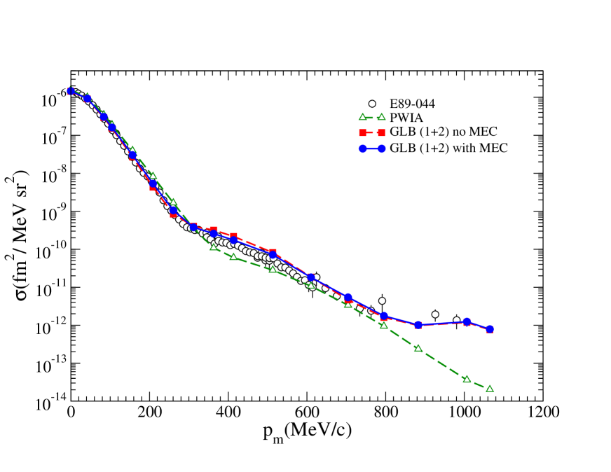
Figure 1: (Color online) Differential cross sections for the ³He($e,e^{\prime}p$)²H reaction at $\phi$=180^∘. The experimental data are compared with the plane-wave-impule-approximation (PWIA), and with the full single and double rescattering Glauber approximation with MEC (GLB(1+2) With MEC) and without MEC (GLB(1+2) No MEC). The profile operator in the Glauber approximation is derived from $NN$ scattering amplitudes (including central, single-spin flip and double-spin flip terms), boosted from the c.m. frame to the rescattering (lab) frame. Statistical Monte Carlo errors are smaller than the symbols, and lines drawn to guide the eye.

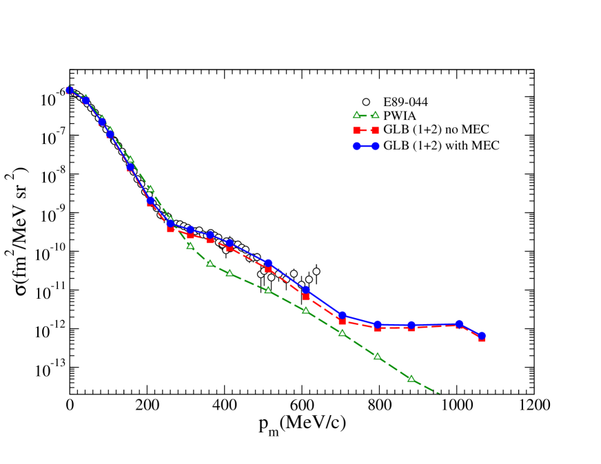
Figure 2: (Color online) Same as Fig. 1, but at $\phi$=0^∘.

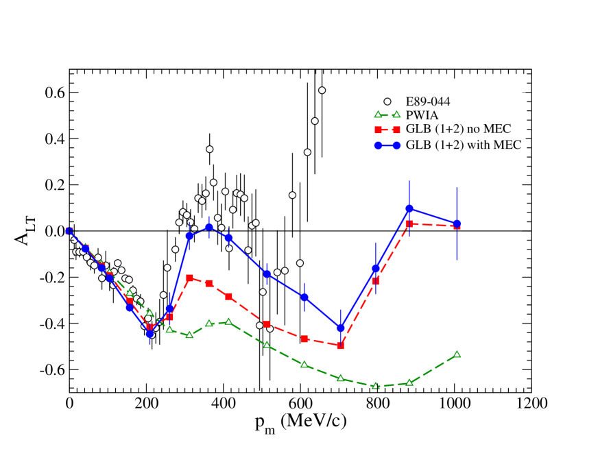
Figure 3: (Color online) Same as Fig. 1, but for the longitudinal-transverse asymmetry.

In Figs. 1–3, the curves labeled PWIA represent the results obtained in the plane-wave impulse-approximation disregarding all FSI. The PWIA overpredicts the data at low $p_{m}$ and underpredicts them at high $p_{m}$. The curves labeled “GLB(1+2) No MEC” represent the results obtained in the Glauber approximation with single and double rescattering, but neglecting contributions from meson exchange currents (MEC). By accounting for FSI, we note a significant improvement in describing the experimental cross-section values. Inclusion of MEC contributions, curves labeled as “GLB(1+2) With MEC”, further improves the comparison with the data. While in Figs. 1 and 2 the MEC effects appear small in comparison to the FSI, it is clear that they improve the predictions, especially at intermediate values of missing momentum. In Fig. 3, where the asymmetry is shown, the effects are even more pronounced. We note again the inability of the PWIA to successfully account for the experimental features, except for very low values of missing momentum. The structure of the data is clearly dominated by FSI as the missing momentum is increased, and the importance of the MEC is again notable. Indeed at intermediate values of $p_{m}$ the MEC contribution is of comparable strength as the FSI. When calculating $A_{LT}$, we are taking a difference between the cross sections shown in Fig. 1 and Fig. 2, where in the former the MEC suppress the results, and in the latter the MEC enhance them. So even though this is a small effect in the individual cross sections, it becomes quite large when taking their difference.

We next want to investigate model-dependent effects due to the $NN$ scattering amplitudes. In order to compare the various effects, calculations were performed for a variety of cases, and comparisons are presented in Figs. 4–8.

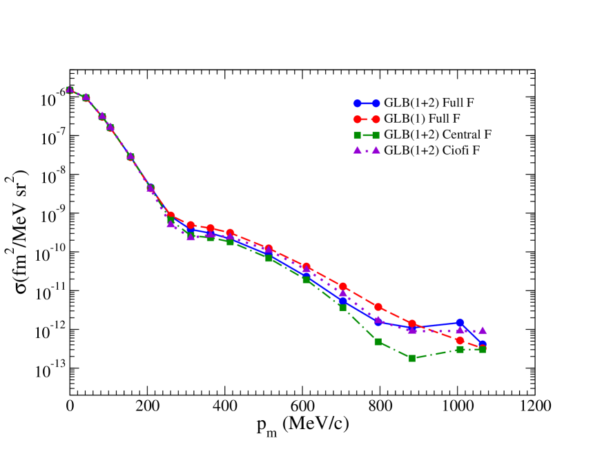
Figure 4: (Color online) Differential cross sections for the ³He($e,e^{\prime}p$)²H reaction at $\phi$=180^∘ obtained in various approximation schemes, see text for descriptions of the approximations. Lines are drawn to guide the eye.

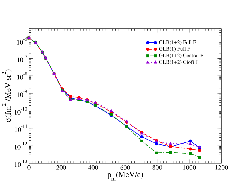
Figure 5: (Color online) Same as Fig. 4, but at $\phi$=0^∘.

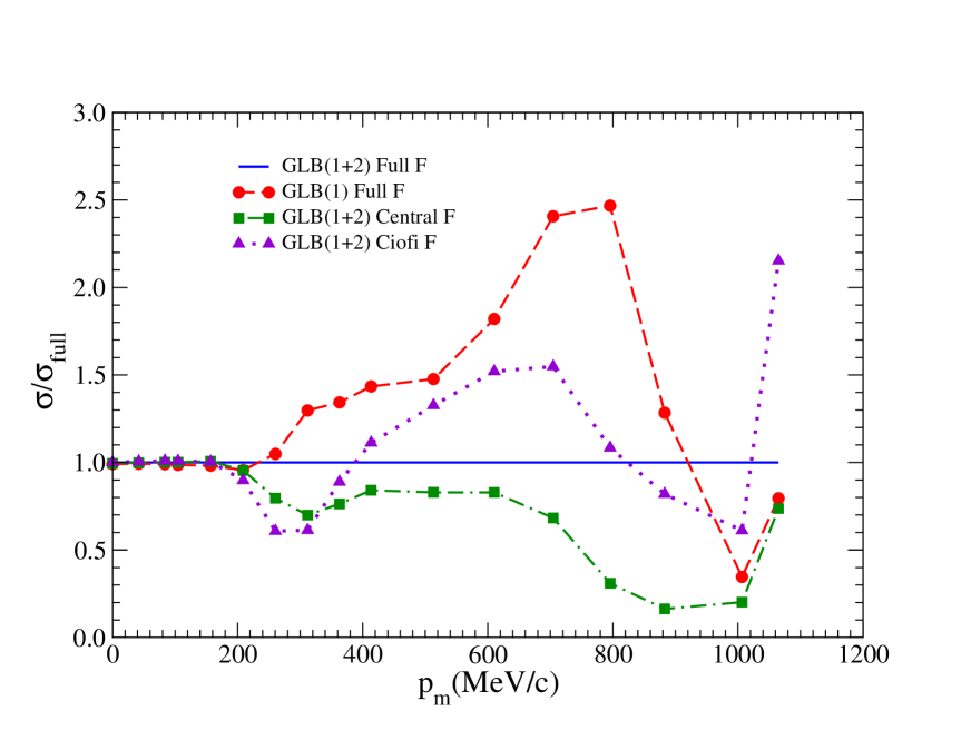
Figure 6: (Color online) Ratios of differential cross sections as shown in Fig. 4.

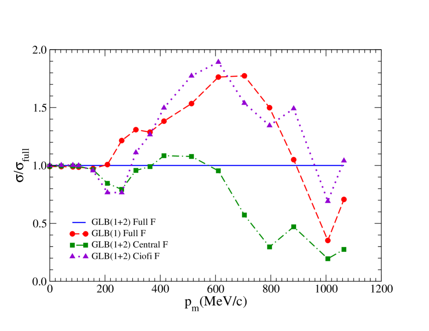
Figure 7: (Color online) Ratios of differential cross sections as shown in Fig. 5.

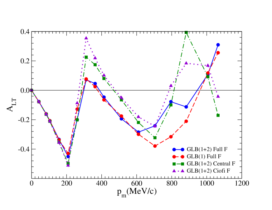
Figure 8: (Color online) Same as Fig. 4, but for the longitudinal-transverse asymmetry.

Specifically, we are interested in quantifying the role of spin dependence in the FSI, which this work facilitates well, since all spin dependence is retained in the Glauber profile operator. These cases were all calculated for the same random walk in the Monte Carlo integration, and are not compared to experimental data. Since we have already investigated MEC contributions and noted their importance in the discussion above, all results below include them. The cases we investigate are:

1. Curves labeled “GLB(1+2) Full F” correspond to the Glauber approximation with single and double rescattering and include the full spin dependence in the $NN$ scattering amplitudes.

2. Curves labeled “GLB(1)” include only single scattering in the Glauber approximation, but still incorporate the full spin dependence in the $NN$ scattering amplitudes.

3. Curves labeled “GLB(1+2) Central F” correspond to Glauber single and double rescattering, but with all spin dependent terms turned off in the $NN$ scattering amplitudes, that is, in Eq. (10) we set $\overline{F}^{\,NN}_{m}(\overline{{\bf k}}^{\,2}\!,s)=0$ for $m$=2–5, so that only the central term $\overline{F}^{\,NN}_{1}(\overline{{\bf k}}^{\,2}\!,s)$ contributes.

4. Curves labeled “GLB(1+2) Ciofi F” correspond to using a common $NN$ parametrization given in Eq. (29), which includes no explicit spin dependence. The parameterization is described in Appendix A. It should be noted, however, that when fitting a spin independent amplitude to experimental data, spin dependence can implicitly enter the parameterization, which causes some ambiguity when trying to determine its role in FSI.

In Figs. 4 and 5 we show the differential cross sections calculated at $\phi$= 180^∘ and $\phi$=0^∘, respectively. Since these are semilog plots, we also plot ratios of the various cases to the full double rescattering, fully spin dependent calculation, case 1. These are shown in Figs. 6 and 7, again for $\phi$=180^∘ and $\phi$=0^∘, respectively. In Fig. 8 we plot the longitudinal-transverse asymmetry for comparison of the four cases. In these figures we first note the necessity of including the double rescattering in the Glauber approximation, case 2. At all but the lowest missing momentum, where FSI are negligible, we see that the single scattering approximation leads to a significant deviation for $p_{m}>200~{}\rm{MeV/c}$. Next we observe the effect of “turning off” the spin dependent contributions the $NN$ amplitudes, case 3. Here again we note significant deviations from the full result. Finally, we turn to case 4 and note similar deviations as in case 3 for $p_{m}\lesssim 400$ MeV/c. However, at larger $p_{m}$ where FSI effects become quite important, predictions for cases 3 and 4 differ significantly from each other—see Figs. 6–7—which can be traced back to differences between the central amplitudes of cases 3 and 4 (see discussion in Appendix A).

It is interesting to point out that for the asymmetry, shown in Fig. 8, the effects are similar for each of the four cases, however, we note that there is no significant deviation for the single and double rescattering up to $p_{m}\approx 600~{}\rm{MeV/c}$. This implies that the effects of double rescattering, so pronounced in the differential cross section for $p_{m}>200~{}\rm{MeV/c}$, cancel when calculating the asymmetry. This is similar to the above discussion regarding MEC, and again is due to taking differences of cross sections, except here the double scattering contribution increases the cross sections for both kinematics so when taking the difference this increase is canceled out.

V.2 ⁴He($e,e^{\prime}p$)³H

We now turn our attention to the observables calculated for the ⁴He($e,e^{\prime}p$)³H reaction. In this case we utilize both the Glauber description of FSI as well as an optical potential. We begin by discussing JLab experiment E97-111, for which preliminary data have been published in Ref. Reitz (2004)—these preliminary data, which only include statistical errors, are shown in the figures below. The experiment measured cross sections for the electrodisintegration of ⁴He into ³H and $p$ clusters in three different kinematic setups. The first setup labeled CQ2, in which the electron momentum and energy transfers were kept fixed at $q\simeq 1.43$ GeV and $\omega\simeq 0.52$ GeV, was in quasi-perpendicular kinematics (with the missing momentum ${\bf p}_{m}$ close to being perpendicular to ${\bf q}$), while the remaining two setups labeled PY1 and PY2 were both in quasi-parallel kinematics (with ${\bf p}_{m}$ close to being parallel to ${\bf q}$) and both covered the same range $0\lesssim p_{m}\lesssim 500$ MeV/c, but the electron beam energy and scattering angle were, respectively, about 2.4 GeV and 16.9^∘ in PY1 and about 3.2 GeV and 18.9^∘ in PY2.

In Figs. 9–11 we show for both experiment and theory the reduced cross section, defined as

$$\sigma^{\rm red}=\frac{1}{p\,E\,f_{\rm rec}\,\sigma_{ep}^{\rm CC1}}\,\frac{d^{5}\sigma}{dE_{e}^{\prime}d\Omega_{e}^{\prime}d\Omega}\ ,$$ (28)

where $\sigma_{ep}^{\rm CC1}$ denotes the CC1 off-shell parameterization of the electron-proton cross section due to deForest de Forest (1983). The various curves are labeled as follows: “PWIA” represents the plane wave impulse approximation, “GLB with (no) MEC” treats FSI in the Glauber approximation with (without) MEC, “OPT with (no) MEC” uses the optical potential to account for FSI with (without) MEC, and finally the experimental data are labeled by the experiment number “E97-111”. We note that the calculations in the Glauber approximation include single, double and triple rescattering (see Sec. II.1).

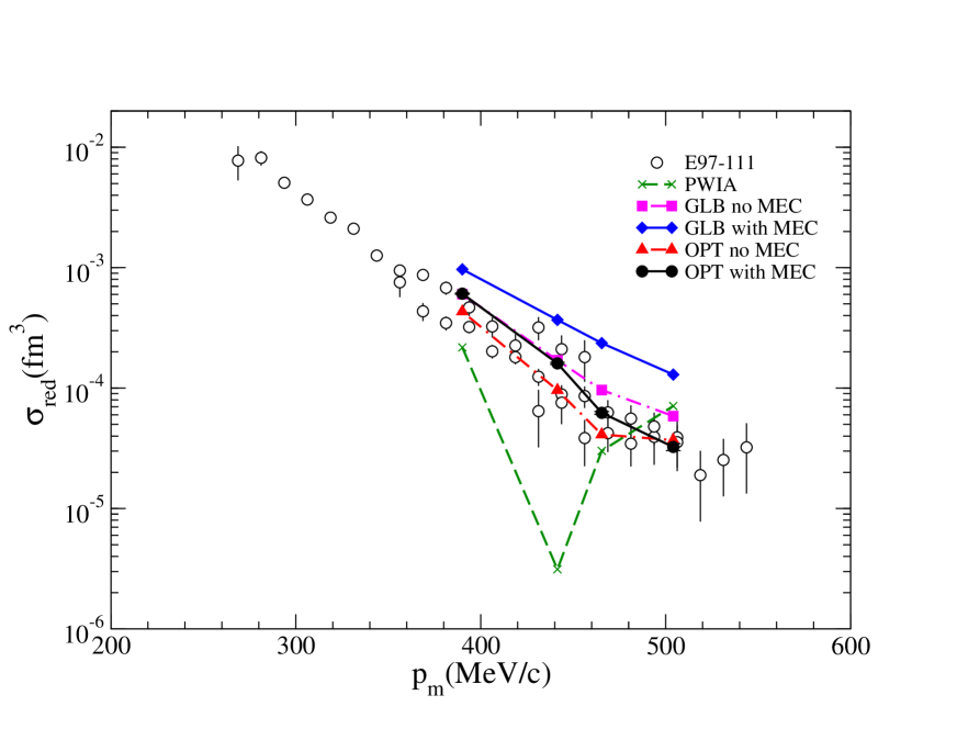
Figure 9: (Color online) Reduced differential cross section of ⁴He($e,e^{\prime}p$)³H compared to experimental data and various calculation schemes. “CQ2” refers to the experimental kinematics. See text for descriptions of the curves. Lines are drawn to guide the eye.

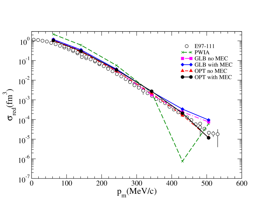
Figure 10: (Color online) Same as Fig. 9 except for “PY1” kinematics.

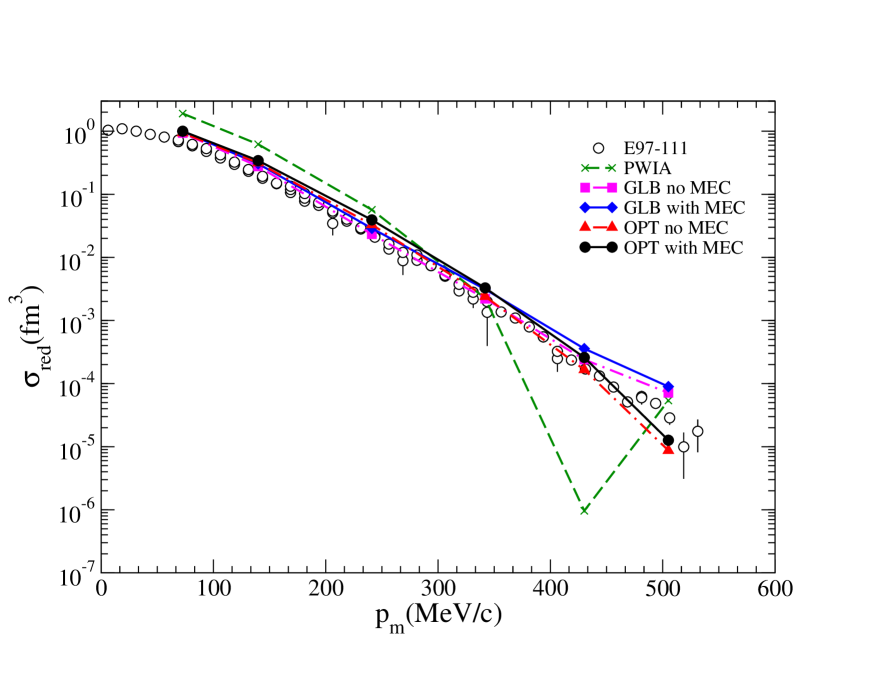
Figure 11: (Color online) Same as Fig. 9 except for “PY2” kinematics.

The three kinematic setups all cover the region of missing momentum close to 450 MeV/c, where the PWIA results are orders of magnitude smaller than the data. In PWIA the cross section is proportional to the $p$-³H cluster momentum distribution, which exhibits a node for $p_{m}$ close to 450 MeV/c Schiavilla et al. (1986); *Wiringa:2013ala. This node is filled in by FSI contributions, which shift PWIA strength from the low $p_{m}$ region to the high $p_{m}$ one, see Figs. 10–11. The contributions from MEC are significant, particularly for kinematics CQ2, and increase the cross section over the whole $p_{m}$ range of interest. The full calculations, including FSI either in the Glauber approximation or via the optical potential and MEC contributions, are in reasonable agreement with data for kinematics PY1 and PY2, although they both tend to overpredict the measured cross sections at low $p_{m}$ (but not as severely as the PWIA calculation). For kinematics CQ2, the “OPT with MEC” calculation provides a satisfactory description of data, while the “GLB with MEC” calculation leads to cross sections which are significantly larger than the measured values. We note that for kinematics CQ2 the relative kinetic energy between the proton and triton clusters is about 0.31 GeV, so well within the range of applicability of the optical potential, which was fitted to $p$-³H scattering data up to relative kinetic energy of 0.45 GeV (Sec. II.2). In contrast, the proton lab kinetic energies for this same kinematic setup are of the order of 0.46 GeV, arguably too low for the validity of the Glauber approximation. For the quasi-parallel kinematics PY1 (PY2) the $p$-³H relative kinetic energies and proton lab kinetic energies are, respectively, in the ranges 0.22–1.05 (0.44–1.55) GeV and 0.34–0.98 (0.51–1.42) GeV, as the missing momentum increases from $\simeq 0.06$ GeV/c to $\simeq 0.5$ GeV/c, and therefore one would expect the treatment of FSI via the optical potential to be valid on the low side of $p_{m}$ and that based on the Glauber approximation to be appropriate for the high side of $p_{m}$. In fact, the actual calculations shown in Figs. 10–11 indicate that the optical potential and Glauber approximation differ significantly only beyond $p_{m}\gtrsim 400$ MeV/c, with the “OPT with MEC” and “GLB with MEC” results, respectively, underestimating and overestimating the data.

We now turn our attention to the polarization observables in the ⁴He$(\vec{e},e^{\prime}\vec{p}\,)^{3}$H reaction. We present the induced polarization $P_{y}$ in Fig. 12, and the super-ratio $(P^{\prime}_{x}/P^{\prime}_{z})/(P^{\prime}_{x}/P^{\prime}_{z})_{\rm PWIA}$ in Fig. 13.

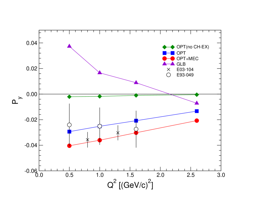
Figure 12: (Color online) Induced polarization for ⁴He compared to experimental data. The optical potential is tuned to reproduce the data. See text for descriptions of the curves. Lines are drawn to guide the eye.

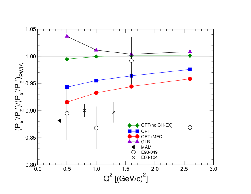
Figure 13: (Color online) Polarization transfer for ⁴He compared to experimental data. See text for descriptions of the curves. Lines are drawn to guide the eye.

These are both plotted versus the four momentum transfer of the virtual photon, $Q^{2}$. These observables are compared with data labeled according to the experiment. In Fig. 12 the data labeled “E03-104” are from Ref. Malace et al. (2011), and “E93-049” are from Ref. Strauch et al. (2003). In Fig. 13 the data labeled “E03-104” are from Ref. Paolone et al. (2010), “E93-049” are from Ref. Strauch et al. (2003), and “MAMI” are from Ref. Dieterich et al. (2001). When comparing to the JLab experimental data we should be mindful that these are averaged over the acceptance of the spectrometers. The super-ratio is only mildly affected by this Strauch , however the induced polarization can vary substantially. According to Ref. Malace et al. (2011) the correction is $\lesssim 20\%$, and additional details of how the correction is made can be found in that work. In the figures, the curves labeled “OPT( no CH-EX)” and “OPT” both use one-body electromagnetic currents, the only difference being that in the “OPT( no CH-EX)” calculation the charge-exchange terms in the optical potential are ignored. The curves labeled “OPT+MEC” include the full optical potential as well as the MEC contributions, while the curves labeled “GLB” correspond to results obtained in the Glauber approximation with one-body currents. The statistical errors associated with the Monte Carlo integrations are only shown for the “OPT+MEC” calculation, they are similar in the other cases. Note that these errors are smaller than those reported in Ref. Schiavilla et al. (2005b) because of the larger number of configurations in the present random walk.

The present calculation differs from that reported in Ref. Schiavilla et al. (2005b) in two respects: i) the spin-orbit term in the optical potential, which is poorly determined Schiavilla et al. (2005b), has been constrained here by fitting the precise induced polarization data obtained in Ref. Malace et al. (2011), and ii) calculations of the super-ratio and induced polarization have also been carried out in the Glauber approximation (including up to triple rescattering). In reference to the calculations based on the optical potential the discussion and ensuing conclusions are similar to those presented in the older study Schiavilla et al. (2005b): i) charge-exchange FSI effects are important, ii) the predicted quenching of the super-ratio relative to one comes about because of these effects and because of MEC contributions, and iii) this quenching is in reasonable agreement with that observed in the older Strauch et al. (2003) as well as in the more recent and accurate Paolone et al. (2010) data.

The “GLB” calculation is at variance with data, particularly at lower $Q^{2}$. While it reproduces the magnitudes of the observables, it has the wrong sign for $P_{y}$ and increases the super-ratio relative to one. However, we note that for the data in the low $Q^{2}$ region the proton lab kinetic energies may be too small for the viability of the Glauber treatment of FSI, for example at $Q^{2}=1$ (GeV/c)² this energy is $\simeq 0.55$ GeV.

VI Conclusions

In this study we have expanded and built upon the work of Refs. Schiavilla et al. (2005a, b), and have calculated observables for the processes ³He($e,e^{\prime}p$)²H and ⁴He($e,e^{\prime}p$)³H. We have updated the $NN$ amplitudes, which describe FSI within a Glauber approximation, to include more realistic parameterizations available from SAID, valid over the entire angular region. In addition to the SAID parameterizations we also implemented a minimal $NN$ amplitude, which includes no spin dependence and is only valid in the forward direction, allowing for a valuable analysis of the $NN$ model dependence entering the calculation. Comparisons were made to available experimental data, and the theoretical results are in good agreement with them.

In the case of the ³He($e,e^{\prime}p$)²H reaction we have compared several model-dependent effects which can affect the results significantly. Among these effects, FSI are of utmost importance. Contributions from MEC, while small in some cases, can play a large role in other observables or kinematical regimes. We also investigated the importance of including both the full spin dependence in the profile operator and double rescattering in the Glauber approximation. Neglecting either of these effects will have a detrimental impact on the calculation.

For the ⁴He($e,e^{\prime}p$)³H reaction we found that the results obtained with either the optical potential or Glauber approximation provide a good description of the data obtained in quasi-parallel kinematics (PY1 and PY2). In contrast, the Glauber results overestimate the data in quasi-perpendicular kinematics (CQ2). In reference to the polarization observables measured in the ⁴He$(\vec{e},e^{\prime}\vec{p}\,)^{3}$H reaction, the Glauber results appear to be severely at variance with data on the induced polarization $P_{y}$ and super-ratio $(P^{\prime}_{x}/P^{\prime}_{z})/(P^{\prime}_{x}/P^{\prime}_{z})_{\rm PWIA}$, particularly at low $Q^{2}$. In contrast, these data are reproduced reasonably well in the calculation based on the optical potential, provided the latter accounts for charge-exchange FSI effects, i.e., the coupling between the $p$-³H and $n$-³He channels.

Appendix A $NN$ scattering amplitudes

This work requires the $NN$ scattering amplitudes as input to describe the FSI. Here we use the $NN$ amplitudes $\overline{F}^{NN}_{m}(s,t)$ from Eq. (10), which are in the Wallace representation Wallace (1981); McNeil et al. (1983b), to produce the profile functions given by Eq. (13). We use a complete set of amplitudes obtained from the SAID analysis and a central (no spin dependence) amplitude from Ciofi and Morita Morita et al. (2002); degli Atti and Kaptari (2005); Ciofi degli Atti and Kaptari (2005); degli Atti and Kaptari (2008); degli Atti et al. (2007); Morita et al. (1987, 1988); Braun et al. (2000); Ciofi degli Atti et al. (2008); Ciofi degli Atti and Morita . Some comments are necessary for each of these choices to clarify their usage in the present work.

It is possible to obtain $NN$ scattering amplitudes in two-dimensional spinor space directly from SAID in the form of the Saclay amplitudes which can be easily related to the Wallace form. The problem with this is that for lab kinetic energies below 350 MeV these are not in agreement with those obtained from the Nijmegen analysis (http://nn-online.org/). However, helicity amplitudes can also be obtained directly from SAID and these can then be converted to Saclay amplitudes, which are in agreement with the Nijmegen analysis. As a result, we start from the SAID helicity amplitudes. These are then converted to the Fermi invariant amplitudes of Eq. (11) as described in Ref. Jeschonnek and Van Orden (2008). The coefficients of the Fermi invariant amplitudes are saved as tables of the five invariant amplitudes and as a function of c.m. angle for laboratory kinetic energies $T_{lab}$ from 0.05 GeV to 1.3 GeV for $pn$ scattering and 0.05 GeV to 3.0 GeV for $pp$ scattering. These tables are interpolated using bicubic splines to obtain scattering amplitudes at any energy and angle within the tabulated energy range. These invariant amplitudes have been used successfully to calculate a number of deuteron electrodisintegration observables Jeschonnek and Van Orden (2008, 2010, 2009). For the current work the Fermi invariants are converted to Wallace amplitudes by multiplication by an appropriate matrix. Some care has to be used in implementing this approach due to a problem with the production of the helicity amplitudes by SAID. In extracting the amplitudes we have specified that at each energy these are given from $\theta_{c.m.}=0^{\circ}$ to $180^{\circ}$ in steps of $5^{\circ}$. The resulting amplitudes show a very strong variation at angles near both endpoints resulting in differential cross sections that have large spikes near $0^{\circ}$ and $180^{\circ}$ that are inconsistent with the scattering data. To eliminate this problem, amplitudes at $5^{\circ}$ and $10^{\circ}$ are replaced by values obtained from a cubic polynomial fixed by data at $0^{\circ}$, $15^{\circ}$, $20^{\circ}$ and $25^{\circ}$. This produces differential cross sections that are in agreement with data.

Ciofi and Morita use only a single spin-independent amplitude of the form

$$\overline{F}^{NN}_{1}(s,\bar{\bm{k}}^{2})=-i\,\sigma_{tot}(s)\left[1-i\alpha(s)\right]{\rm e}^{-\beta\,\bar{\bm{k}}^{2}}$$ (29)

where $\sigma_{tot}$ is the total $NN$ cross section, $\alpha$ is a ratio of the real to imaginary part of the forward scattering amplitude (often referred to as $\rho$) and $\beta$ is determined by calculating the total elastic cross section from Eq. (29) giving

$$\beta=\frac{\sigma_{tot}^{2}(s)}{32\pi\,\sigma_{el}^{2}(s)}\left[1+\alpha^{2}(s)\right]\,.$$ (30)

The quantities $\sigma_{tot}$, $\alpha=\rho$ and $\sigma_{el}$ can be obtained from either the PDG or from SAID. Differential cross sections using the SAID and Ciofi amplitudes are shown for $pn$ scattering in Fig. 14(a) and for $pp$ scattering in Fig. 14(b) for the full kinematically allowed range in $t=-\bar{\bm{k}}^{2}$.

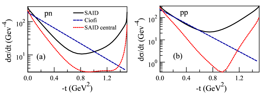
Figure 14: (color online) Differential cross sections obtained from the SAID (solid line), Ciofi (dashed line) and the central contribution from SAID (short dashed line) amplitudes for (a) $pn$ scattering and (b) $pp$ scattering for $T_{lab}=0.8\ {\rm GeV}$ ($s=5.03\ {\rm GeV^{2}}$).

Note that while the SAID and Ciofi results are similar in the forward direction for $pp$ scattering, this is not the case for $pn$ scattering. The problem here is in determining $\beta$. The total elastic cross section for $pp$ scattering is completely described by integrating from $0^{\circ}$ to $90^{\circ}$ since for indistinguishable protons each scattering in the c.m. frame will result in one proton in the forward direction and one in the backward direction. This is not the case for $pn$ scattering since a forward scattering proton will be associated with a backward scattering neutron and a backward scattering proton will be associated with a forward scattering neutron. The total elastic $pn$ cross section requires integration from $0^{\circ}$ to $180^{\circ}$. In the case of Fig. 14(b) the total $pp$ elastic cross section corresponds to integrating the differential cross section over half of the range in $t$, while for Fig. 14(a) the total $pn$ elastic cross section corresponds to integrating the differential cross section over the complete range in $t$. By including the contributions from backward scattering protons, the total $pn$ elastic cross section is larger than would be required to fit the data in the forward direction resulting in a smaller value of $\beta$ as given by Eq. (30). Note also that the values of the cross section calculated from the Ciofi amplitudes are smaller than those obtained from the SAID amplitudes at $t=0$ due to the contributions from spin-dependent amplitudes at this point.

The third calculation shown in Figs. 14(a) and 14(b) shows the contribution of only the central part of the SAID amplitudes to the differential cross section. This clearly shows that the spin-dependent amplitudes provide a significant part of the cross section and that the method used by Ciofi transfers part of this strength into the central amplitude.

Fortran90 modules are available from Ford and Van Orden (FVO) which calculate the invariant functions, ${\cal F}_{m}^{NN}(s,t)$, given in Eq. (11). The subroutines can provide the amplitudes for a variety of models depending on the energies desired as well as the complexity of the model. At a basic level there is a parametrization available from Ciofi and Morita Morita et al. (2002); degli Atti and Kaptari (2005); Ciofi degli Atti and Kaptari (2005); degli Atti and Kaptari (2008); degli Atti et al. (2007); Morita et al. (1987, 1988); Braun et al. (2000); Ciofi degli Atti et al. (2008); Ciofi degli Atti and Morita describing the $NN$ system with a single amplitude with no spin dependence. Using this amplitude provides a useful comparison for studying how the FSI model dependence, specifically spin dependence, contributes to a calculation. Next one can choose the Wallace parametrization Wallace (1981), which incorporates spin dependence, but is only valid at small angles. This model was utilized in an earlier work Schiavilla et al. (2005a) but, due to the limitation above, is not used in this work. There are two parametrizations available which include all spin dependence and are valid over the entire angular region. These are the SAID model Arndt et al. (2000, 2007); SAI valid for $s<5.4$ (GeV²), and a Regge model Ford and Van Orden (2013) valid for $s>5.4$ (GeV²). In this work we consider all spin dependence of the FSI, and the energies of interest are those of the SAID approach. For all models the amplitudes are converted first into Fermi invariant functions with a consistent normalization. The Fermi invariants from any model can be used directly or converted to helicity amplitudes, Saclay amplitudes or Wallace amplitudes.

As discussed above, for the SAID analysis the five independent helicity amplitudes can be obtained on a tabulated grid for the c.m. energy ($\overline{E}$) and angle ($\overline{\theta}$). For convenience we work with the Mandelstam variables which are related to the $NN$ c.m. energy and angle by

$$s =4\overline{E}^{2}$$ (31)

$$t =-\overline{{\bf k}}^{2}=-\frac{s-4\,m^{2}}{2}[1-\cos(\overline{\theta})].$$ (32)

If the amplitudes are extracted in units of fm there is a normalization relation between the SAID and FVO conventions,

$$T^{FVO}_{\lambda^{\prime}_{1},\lambda^{\prime}_{2};\lambda_{1},\lambda_{2}}(s,t)=-\frac{4\pi\sqrt{s}}{\hbar c\,m^{2}}T^{SAID}_{\lambda^{\prime}_{1},\lambda^{\prime}_{2};\lambda_{1},\lambda_{2}}(s,t)$$ (33)

The invariants can then be obtained using,

$$\left(\begin{array}[]{c}{\cal F}^{NN}_{S}(s,t)\\ {\cal F}^{NN}_{V}(s,t)\\ {\cal F}^{NN}_{T}(s,t)\\ {\cal F}^{NN}_{P}(s,t)\\ {\cal F}^{NN}_{A}(s,t)\end{array}\right)=\frac{1}{s-4\,m^{2}}{M^{HtoI}}\left(\begin{array}[]{l}T_{\frac{1}{2},\frac{1}{2};\frac{1}{2},\frac{1}{2}}(s,t)\\ T_{\frac{1}{2},\frac{1}{2};\frac{1}{2},-\frac{1}{2}}(s,t)\\ T_{\frac{1}{2},-\frac{1}{2};\frac{1}{2},-\frac{1}{2}}(s,t)\\ T_{\frac{1}{2},\frac{1}{2};-\frac{1}{2},-\frac{1}{2}}(s,t)\\ T_{\frac{1}{2},-\frac{1}{2};-\frac{1}{2},\frac{1}{2}}(s,t)\end{array}\right),$$ (34)

where the matrix $M^{HtoI}$ and additional details of this discussion can be found in the Appendix of Ref. Jeschonnek and Van Orden (2008).

Once the invariant functions are obtained we need to represent the amplitudes in the Wallace form so that the Glauber profile operator can be calculated. Normalization between the FVO convention and the convention used in this work is given as,

$$T_{\lambda^{\prime}_{1},\lambda^{\prime}_{2};\lambda_{1},\lambda_{2}}(s,t)=\frac{i\hbar c\,m^{2}}{2\pi\sqrt{s(s-4\,m^{2})}}T^{FVO}_{\lambda^{\prime}_{1},\lambda^{\prime}_{2};\lambda_{1},\lambda_{2}}(s,t)$$ (35)

It is straightforward to transform from the invariant functions to the Wallace form via another matrix multiplication,

$$\left(\begin{array}[]{c}\overline{F}^{NN}_{1}(s,t)\\ \overline{F}^{NN}_{2}(s,t)\\ \overline{F}^{NN}_{3}(s,t)\\ \overline{F}^{NN}_{4}(s,t)\\ \overline{F}^{NN}_{5}(s,t)\end{array}\right)=\frac{i\hbar c\,m^{2}}{2\pi\sqrt{s(s-4\,m^{2})}}M^{ItoW}\left(\begin{array}[]{c}{\cal F}^{NN}_{S}(s,t)\\ {\cal F}^{NN}_{V}(s,t)\\ {\cal F}^{NN}_{T}(s,t)\\ {\cal F}^{NN}_{P}(s,t)\\ {\cal F}^{NN}_{A}(s,t)\end{array}\right),$$ (36)

where the matrix $M^{ItoW}$ is given below and was obtained from McNeil et al. (1983b). In Appendix B we show how these amplitudes can be boosted to the rescattering frame (which is in practice taken as the lab frame, see discussion in Sec. II.1), and the profile operator can then be calculated from the boosted amplitudes. The matrix elements are:

$$M^{ItoW}_{11} =\frac{(-4m^{2}-2m\sqrt{s}+t)^{2}}{4m^{2}(2m+\sqrt{s})^{2}}$$

$$M^{ItoW}_{12} =\frac{(-16m^{4}-16m^{3}\sqrt{s}+2s^{2}+3st+t^{2}+4m^{2}(s+t)+8m\sqrt{s}(s+t))}{4m^{2}(2m+\sqrt{s})^{2}}$$

$$M^{ItoW}_{13} =\frac{t(4m\sqrt{s}+2s+t)}{2m^{2}(2m+\sqrt{s})^{2}}$$

$$M^{ItoW}_{14} =0$$

$$M^{ItoW}_{15} =\frac{(4m^{2}-s-t)t}{4m^{2}(2m+\sqrt{s})^{2}}$$

$$M^{ItoW}_{21} =\frac{t(-4m^{2}+s+t)}{4m^{2}(2m+\sqrt{s})^{2}}$$

$$M^{ItoW}_{22} =\frac{t(4m\sqrt{s}+2s+t)}{4m^{2}(2m+\sqrt{s})^{2}}$$

$$M^{ItoW}_{23} =\frac{-16m^{4}-16m^{3}\sqrt{s}+2s^{2}+3st+t^{2}+4m^{2}(s+t)+8m\sqrt{s}(s+t)}{2m^{2}(2m+\sqrt{s})^{2}}$$

$$M^{ItoW}_{24} =0$$

$$M^{ItoW}_{25} =-\frac{(-4m^{2}-2m\sqrt{s}+t)^{2}}{4m^{2}(2m+\sqrt{s})^{2}}$$

$$M^{ItoW}_{31} =\frac{(4m^{2}+2m\sqrt{s}-t)\sqrt{-4m^{2}+s+t}}{4m^{2}(2m+\sqrt{s})^{2}}$$

$$M^{ItoW}_{32} =-\frac{(4m^{2}+6m\sqrt{s}+2s+t)\sqrt{-4m^{2}+s+t}}{4m^{2}(2m+\sqrt{s})^{2}}$$

$$M^{ItoW}_{33} =-\frac{(4m^{2}+6m\sqrt{s}+2s+t)\sqrt{-4m^{2}+s+t}}{2m^{2}(2m+\sqrt{s})^{2}}$$

$$M^{ItoW}_{34} =0$$

$$M^{ItoW}_{35} =\frac{(-4m^{2}-2m\sqrt{s}+t)\sqrt{-4m^{2}+s+t}}{4m^{2}(2m+\sqrt{s})^{2}}$$

$$M^{ItoW}_{41} =\frac{-4m^{2}+s+t}{4m^{2}(2m+\sqrt{s})^{2}}$$

$$M^{ItoW}_{42} =\frac{4m\sqrt{s}+2s+t}{4m^{2}(2m+\sqrt{s})^{2}}$$

$$M^{ItoW}_{43} =\frac{4m\sqrt{s}+2s+t}{2m^{2}(2m+\sqrt{s})^{2}}$$

$$M^{ItoW}_{44} =-\frac{1}{4m^{2}}$$

$$M^{ItoW}_{45} =\frac{8m^{2}+4m\sqrt{s}-t}{4m^{2}(2m+\sqrt{s})^{2}}$$

$$M^{ItoW}_{51} =\frac{(4m^{2}-s-t)t}{4m^{2}(2m+\sqrt{s})^{2}}$$

$$M^{ItoW}_{52} =\frac{(4m^{2}-s-t)t}{4m^{2}(2m+\sqrt{s})^{2}}$$

$$M^{ItoW}_{53} =-\frac{-32m^{4}-32m^{3}\sqrt{s}+2s^{2}+4m^{2}t+3st+t^{2}+8m\sqrt{s}(s+t)}{2m^{2}(2m+\sqrt{s})^{2}}$$

$$M^{ItoW}_{54} =0$$

$$M^{ItoW}_{55} =\frac{32m^{4}+32m^{3}\sqrt{s}-2s^{2}-12m^{2}t-st+t^{2}-8m\sqrt{s}(s+t)}{4m^{2}(2m+\sqrt{s})^{2}}\ .$$ (37)

Appendix B From the c.m. to the lab frame

The elastic scattering amplitude in the lab frame is written as

$$(2{\rm i}\,p)^{-1}\,F^{NN}_{ij}({\bf k},s)=\sum_{m=1}^{8}F^{NN}_{m}(s,{\bf k}^{\,2})O^{m}_{ij}\ ,$$ (38)

where the eight operators $O^{m}_{ij}$ are taken as

$$O^{\,m=1,\dots,8}_{ij}=1\,,\,{\bm{\sigma}}_{i}\cdot{\bm{\sigma}}_{j}\,,\,{\rm i}\,{\bm{\sigma}}_{i}\cdot{\bf k}\times\hat{\bf p}\,,\,{\rm i}\,{\bm{\sigma}}_{j}\cdot{\bf k}\times\hat{\bf p}\,,\,{\bm{\sigma}}_{i}\cdot{\bf k}\,{\bm{\sigma}}_{j}\cdot{\bf k}\,,\,{\bm{\sigma}}_{i}\cdot\hat{\bf p}\,{\bm{\sigma}}_{j}\cdot\hat{\bf p}\,,\,i\,{\bm{\sigma}}_{i}\cdot{\bf k}\,{\bm{\sigma}}_{j}\cdot\hat{\bf p}\,,\,i\,{\bm{\sigma}}_{i}\cdot\hat{\bf p}\,{\bm{\sigma}}_{j}\cdot{\bf k}\ .$$ (39)

Here ${\bf p}$ is the momentum of the initial fast nucleon and in the eikonal limit the momentum transfer ${\bf k}$ is perpendicular to ${\bf p}$. The functions $F^{NN}_{m=1,\dots,8}$ are then obtained as linear combinations of the invariant functions ${\cal F}_{m=1,\dots,5}^{NN}$,

$$F^{NN}_{m}=\sum_{n=1}^{5}L_{mn}\,{\cal F}^{NN}_{n}\ ,$$ (40)

where the 8$\times$5 matrix $L$ is given by

$L=\left[\begin{array}[]{ccccc}1-\frac{p^{2}}{w_{p}w_{p-k}}&1+\frac{p^{2}}{w_{p}w_{p-k}}+\frac{k^{2}}{w_{p-k}w_{k}}&-\frac{2k^{2}}{w_{p-k}w_{k}}&0&0\\ 0&-\frac{k^{2}}{w_{p-k}w_{k}}&2\left(1+\frac{p^{2}}{w_{p}w_{p-k}}+\frac{k^{2}}{w_{p-k}w_{k}}\right)&0&-1+\frac{p^{2}}{w_{p}w_{p-k}}\\ \frac{p}{w_{p}w_{p-k}}&-\frac{p}{w_{p}w_{p-k}}\left(1+\frac{w_{-}}{w_{k}}\right)&-\frac{2p}{w_{p}w_{p-k}}\frac{w_{+}}{w_{k}}&0&0\\ 0&-\frac{p}{w_{p}w_{p-k}}\frac{w_{+}}{w_{k}}&-\frac{2p}{w_{p}w_{p-k}}\left(1+\frac{w_{-}}{w_{k}}\right)&0&-\frac{p}{w_{p}w_{p-k}}\\ 0&\frac{1}{w_{p-k}w_{k}}&-\frac{2}{w_{p-k}w_{k}}&-\frac{1}{w_{p-k}w_{k}}&-\frac{1}{w_{p-k}w_{k}}\\ 0&0&-\frac{4p^{2}}{w_{p}w_{p-k}}&0&-\frac{2p^{2}}{w_{p}w_{p-k}}\\ 0&-i\frac{p}{w_{p}w_{p-k}}\frac{w_{-}}{w_{k}}&-i\frac{2p}{w_{p}w_{p-k}}\left(1+\frac{w_{+}}{w_{k}}\right)&0&-i\frac{p}{w_{p}w_{p-k}}\\ 0&0&-i\frac{2p}{w_{p}w_{p-k}}&-i\frac{p}{w_{p}w_{p-k}}\frac{w_{-}}{w_{k}}&-i\frac{p}{w_{p}w_{p-k}}\left(1+\frac{w_{+}}{w_{k}}\right)\end{array}\right]\ ,$

and the factors $E_{q}$ and $w_{q}$ are defined as $E_{q}\equiv\sqrt{{\bf q}^{2}+m^{2}}$ and $w_{q}\equiv E_{q}+m$, with ${\bf q}={\bf p}$, ${\bf k}$, ${\bf p}-{\bf k}$, and $w_{\pm}\equiv w_{p-k}\pm w_{p}$,

The $N$$N$ profile operator $\Gamma^{NN}_{ij}$ is obtained from Eq. (13) by replacing $\Gamma^{(m)}_{ij}$ with $\Gamma^{(m)}_{NN}$ for $m=1,\dots,8$. The functions $\Gamma^{(m)}_{NN}$ are in turn derived from Bessel transforms of the $F^{NN}_{m}$ amplitudes. We find:

$$\Gamma^{(m)}_{NN}(b;s)=2\,p^{2}\int_{-1}^{1}{\rm d}x\,J_{0}(kb)\,F^{NN}_{m}(k^{2};s)$$ (41)

for $m=1,6$;

$$\Gamma^{(m)}_{NN}(b;s)=\frac{2\,p^{2}}{b}\int_{-1}^{1}{\rm d}x\,k\,J_{1}(kb)\,F^{NN}_{m}(k^{2};s)$$ (42)

for $m=3,4,7,8$; and lastly

$$\Gamma^{(2)}_{NN}(b;s) = 2\,p^{2}\int_{-1}^{1}{\rm d}x\,J_{0}(kb)\,F^{NN}_{2}(k^{2};s)+\frac{2\,p^{2}}{b}\int_{-1}^{1}{\rm d}x\,k\,J_{1}(kb)\,F^{NN}_{5}(k^{2};s)\ ,$$ (43)

$$\Gamma^{(5)}_{NN}(b;s) = \frac{2\,p^{2}}{b^{2}}\int_{-1}^{1}{\rm d}x\,k^{2}\,\left[J_{0}(kb)-\frac{2}{k\,b}J_{1}(kb)\right]\,F^{NN}_{5}(k^{2};s)\ .$$ (44)

In obtaining the integrals above, we made the variable change $k\rightarrow 2\,p\,{\rm sin}(\theta/2)=2\,p\,\sqrt{(1-x)/2}$ with $x={\rm cos}\,\theta$.

References

- Rvachev et al. (2005) M. M. Rvachev et al. (Jefferson Lab Hall A Collaboration), Phys. Rev. Lett. 94, 192302 (2005).
- Reitz (2004) B. Reitz (for the Jefferson Lab Hall A Collaboration), Eur. Phys. J. A19, S1, 165 (2004).
- Strauch et al. (2003) S. Strauch et al., Phys. Rev. Lett. 91, 052301 (2003).
- Paolone et al. (2010) M. Paolone et al. (E03-104 Collaboration), Phys. Rev. Lett. 105, 072001 (2010).
- Malace et al. (2011) S. P. Malace et al. (E03-104 Collaboration), Phys. Rev. Lett. 106, 052501 (2011).
- degli Atti and Kaptari (2005) C. C. degli Atti and L. P. Kaptari, Phys. Rev. C 71, 024005 (2005).
- Ciofi degli Atti and Kaptari (2005) C. Ciofi degli Atti and L. P. Kaptari, Phys. Rev. Lett. 95, 052502 (2005).
- degli Atti and Kaptari (2008) C. C. degli Atti and L. P. Kaptari, Phys. Rev. Lett. 100, 122301 (2008).
- Alvioli et al. (2010) M. Alvioli, C. C. d. Atti, and L. P. Kaptari, Phys. Rev. C 81, 021001 (2010).
- Laget (2005a) J. M. Laget, Phys. Rev. C 72, 024001 (2005a).
- Laget (2005b) J. Laget, Physics Letters B 609, 49 (2005b).
- Sargsian et al. (2005a) M. M. Sargsian, T. V. Abrahamyan, M. I. Strikman, and L. L. Frankfurt, Phys. Rev. C 71, 044614 (2005a).
- Sargsian et al. (2005b) M. M. Sargsian, T. V. Abrahamyan, M. I. Strikman, and L. L. Frankfurt, Phys. Rev. C 71, 044615 (2005b).
- Schiavilla et al. (2005a) R. Schiavilla, O. Benhar, A. Kievsky, L. Marcucci, and M. Viviani, Phys.Rev. C72, 064003 (2005a).
- Schiavilla et al. (2005b) R. Schiavilla, O. Benhar, A. Kievsky, L. Marcucci, and M. Viviani, Phys.Rev.Lett. 94, 072303 (2005b).
- Wiringa et al. (1995) R. B. Wiringa, V. G. J. Stoks, and R. Schiavilla, Phys. Rev. C 51, 38 (1995).
- Pudliner et al. (1995) B. S. Pudliner, V. R. Pandharipande, J. Carlson, and R. B. Wiringa, Phys. Rev. Lett. 74, 4396 (1995).
- Arndt et al. (2000) R. A. Arndt, I. I. Strakovsky, and R. L. Workman, Phys. Rev. C 62, 034005 (2000).
- Arndt et al. (2007) R. A. Arndt, W. J. Briscoe, I. I. Strakovsky, and R. L. Workman, Phys.Rev. C76, 025209 (2007).
- (20) “SAID,” http://gwdac.phys.gwu.edu/, accessed: 2012-09-21.
- Wallace (1981) S. Wallace, Advances in Nuclear Physics, edited by J. Negele and E. Vogt, Vol. 12 (Plenum, New York, 1981) p. 135.
- Glauber (1959) R. Glauber, Lectures in Theoretical Physics, edited by W. Brittain and L. Dunham, Vol. 1. (Interscience, New York, 1959).
- McNeil et al. (1983a) J. A. McNeil, L. Ray, and S. J. Wallace, Phys. Rev. C 27, 2123 (1983a).
- van Oers et al. (1982) W. T. H. van Oers, B. T. Murdoch, B. K. S. Koene, D. K. Hasell, R. Abegg, D. J. Margaziotis, M. B. Epstein, G. A. Moss, L. G. Greeniaus, J. M. Greben, J. M. Cameron, J. G. Rogers, and A. W. Stetz, Phys. Rev. C 25, 390 (1982).
- Schiavilla (1990) R. Schiavilla, Phys. Rev. Lett. 65, 835 (1990).
- Viviani et al. (2005) M. Viviani, A. Kievsky, and S. Rosati, Phys. Rev. C 71, 024006 (2005).
- Jeschonnek and Donnelly (1998) S. Jeschonnek and T. W. Donnelly, Phys. Rev. C 57, 2438 (1998).
- Carlson and Schiavilla (1998) J. Carlson and R. Schiavilla, Rev. Mod. Phys. 70, 743 (1998).
- Carlson et al. (2002) J. Carlson, J. Jourdan, R. Schiavilla, and I. Sick, Phys. Rev. C 65, 024002 (2002).
- Marcucci et al. (2005) L. E. Marcucci, M. Viviani, R. Schiavilla, A. Kievsky, and S. Rosati, Phys. Rev. C 72, 014001 (2005).
- Hohler et al. (1976) G. Hohler, E. Pietarinen, I. Sabba Stefanescu, F. Borkowski, G. Simon, et al., Nucl.Phys. B114, 505 (1976).
- Brash et al. (2002) E. J. Brash, A. Kozlov, S. Li, and G. M. Huber, Phys. Rev. C 65, 051001 (2002).
- Jones et al. (2000) M. K. Jones et al. ((The Jefferson Lab Hall A Collaboration)), Phys. Rev. Lett. 84, 1398 (2000).
- Raskin and Donnelly (1989) A. Raskin and T. Donnelly, Annals of Physics 191, 78 (1989).
- Picklesimer and Van Orden (1989) A. Picklesimer and J. W. Van Orden, Phys. Rev. C 40, 290 (1989).
- de Forest (1983) T. de Forest, Jr., Nuclear Physics A 392, 232 (1983).
- Schiavilla et al. (1986) R. Schiavilla, V. Pandharipande, and R. Wiringa, Nuclear Physics A 449, 219 (1986).
- Wiringa et al. (2013) R. Wiringa, R. Schiavilla, S. C. Pieper, and J. Carlson, (2013), arXiv:1309.3794 [nucl-th] .
- Dieterich et al. (2001) S. Dieterich et al., Physics Letters B 500, 47 (2001).
- (40) S. Strauch, Private Communication.
- McNeil et al. (1983b) J. A. McNeil, L. Ray, and S. J. Wallace, Phys. Rev. C 27, 2123 (1983b).
- Morita et al. (2002) H. Morita, M. Braun, C. C. degli Atti, and D. Treleani, Nuclear Physics A 699, 328 (2002), 3rd Int. Conf. on Perspectives in Hadronic Physics.
- degli Atti et al. (2007) C. C. degli Atti, L. Kaptari, and H. Morita, Nuclear Physics A 782, 191 (2007), proceedings of the 5th International Conference on Perspectives in Hadron Physics, Particle–Nucleus and Nucleus–Nucleus Scattering at Relativistic Energies.
- Morita et al. (1987) H. Morita, Y. Akaishi, O. Endo, and H. Tanaka, Progress of Theoretical Physics 78, 1117 (1987).
- Morita et al. (1988) H. Morita, Y. Akaishi, and H. Tanaka, Progress of Theoretical Physics 79, 1279 (1988).
- Braun et al. (2000) M. A. Braun, C. Ciofi degli Atti, and D. Treleani, Phys. Rev. C 62, 034606 (2000).
- Ciofi degli Atti et al. (2008) C. Ciofi degli Atti, L. P. Kaptari, and H. Morita, Few-Body Systems 43, 39 (2008).
- (48) C. Ciofi degli Atti and H. Morita, Private Communication.
- Jeschonnek and Van Orden (2008) S. Jeschonnek and J. W. Van Orden, Phys.Rev. C78, 014007 (2008).
- Jeschonnek and Van Orden (2010) S. Jeschonnek and J. W. Van Orden, Phys.Rev. C81, 014008 (2010).
- Jeschonnek and Van Orden (2009) S. Jeschonnek and J. W. Van Orden, Phys.Rev. C80, 054001 (2009).
- Ford and Van Orden (2013) W. P. Ford and J. W. Van Orden, Phys. Rev. C 87, 014004 (2013).