Transient times, resonances and drifts of attractors in dissipative rotational dynamics

Abstract

In a dissipative system the time to reach an attractor is often influenced by the peculiarities of the model and in particular by the strength of the dissipation. In particular, as a dissipative model we consider the spin–orbit problem providing the dynamics of a triaxial satellite orbiting around a central planet and affected by tidal torques. The model is ruled by the oblateness parameter of the satellite, the orbital eccentricity, the dissipative parameter and the drift term. We devise a method which provides a reliable indication on the transient time which is needed to reach an attractor in the spin–orbit model; the method is based on an analytical result, precisely a suitable normal form construction. This method provides also information about the frequency of motion. A variant of such normal form used to parametrize invariant attractors provides a specific formula for the drift parameter, which in turn yields a constraint - which might be of interest in astronomical problems - between the oblateness of the satellite and its orbital eccentricity.

Keywords. Spin–orbit problem, transient time, dissipative system, attractor.

1 Introduction

We consider a nearly–integrable dissipative system describing the motion of a non–rigid satellite under the gravitational influence of a planet. The motion of the satellite is assumed to be Keplerian; the spin–axis is perpendicular to the orbit plane and it coincides with the axis whose moment of inertia is maximum. The non–rigidity of the satellite induces a tidal torque provoking a dissipation of the mechanical energy. The dissipation depends upon a dissipative parameter and a drift term. If the dissipation were absent, the system becomes nearly–integrable with the perturbing parameter representing the equatorial oblateness of the satellite. The overall model depends also on the orbital eccentricity of the Keplerian ellipse. This problem is often known as the dissipative spin–orbit model and it has been extensively studied in the literature (see, e.g., [5], [7], [22]).

The spin–orbit model exhibits different kinds of attractors, e.g. periodic, quasi–periodic and strange attractors (compare with [1], [2], [9], [15]). As it often happens in dissipative system, the dynamics evolves in such a way that the attractor is reached after an initial transient regime of motion. The prediction of the transient time to reach the attractor is often quite difficult (see, e.g., [18], [19]), but it is obviously of pivotal importance to test the reliability of the result (think, e.g., to the problem of deciding about the convergence of the Lyapunov exponents). The first goal of this paper is to give a recipe which allows to decide the length of the transient time, namely the time needed to go over the transient regime and to settle the system into its typical behavior. Our study is based on the construction of a suitable normal form for dissipative vector fields (see [8], compare also with [13], [16], [20], [24]) that generalizes Hamiltonian normal forms that are usually implemented around elliptic equilibria (see [14]). We compute the frequency in the normalized variables and use it - as well as its back–transformation to the original variables - for a comparison with a numerical integration of the equations of motion. Several experiments are performed as the strength of the dissipation is varied. It should be kept in mind that in dissipative systems one has to tune the drift parameter in order to get specific attractors, since it does not suffice to modify the initial conditions like in the conservative case ([3], [6]). A different formulation of the normal form, precisely a suitable parametric representation of invariant attractors, allows to obtain an explicit form for the drift on the attractor. Taking advantage of the physical definition of the drift term, precisely as a function of the eccentricity ([23], see also [11]), one can derive interesting conclusions on a link between the oblateness parameter and the eccentricity associated to a given invariant attractor. We believe that this constraint might be useful in concrete astronomical applications.

This paper is organized as follows. In Section 2 we present the equations of motion of the spin–orbit problem in the conservative and dissipative cases. The construction of the normal form is developed in Section 3, while the parametric representation of invariant attractors is provided in Section 4. The investigation of the transient time and the analysis of the drift term are performed in Section 5. Some conclusions are drawn in Section 6.

2 The spin–orbit problem with tidal torque

In this Section we describe the spin–orbit model, providing the equation of motion in the conservative case (Section 2.1) and under the effect of a tidal torque, due to the internal non–rigidity of the satellite (Section 2.2).

2.1 The conservative spin–orbit problem

The spin–orbit model describes the dynamics of a rigid body with mass $m$, say $\mathcal{S}$, that we assume to have a triaxial structure with principal moments of inertia $I_{1}\leq I_{2}\leq I_{3}$. The satellite $\mathcal{S}$ moves under the gravitational effect of a perturbing body $\mathcal{P}$ with mass $M$. Moreover, we make the following assumptions:

• the body $\mathcal{S}$ orbits on a Keplerian ellipse around $\mathcal{P}$; we denote by $a$ and $e$ the corresponding semimajor axis and eccentricity;

• the rotation axis of $\mathcal{S}$ is assumed to coincide with the direction of the largest principal axis of inertia;

• the spin–axis is assumed to be aligned with the orbit normal;

• all other perturbations, including dissipative effects, are neglected.

In order to simplify the notation, we normalize the units of measure; precisely, the mean motion ${{{\mathcal{G}}M}\over a^{3}}$ (where ${\mathcal{G}}$ is the gravitational constant) is normalized to one. An important role is played by the following quantity, which is named the equatorial ellipticity:

$$\varepsilon\equiv{3\over 2}{{I_{2}-I_{1}}\over I_{3}}\ .$$

To describe the rotation of $\mathcal{S}$ with respect to $\mathcal{P}$, we introduce the angle $x$ spanned by the largest physical axis (that we assume to lie in the orbital plane) with the perihelion line (see Figure 1).

The Hamiltonian function describing the spin–orbit model under the assumptions $i)$-$iv)$ is (see [5])

$${\mathcal{H}}(y,x,t)={{y^{2}}\over{2}}-{\varepsilon\over 2}({a\over r})^{3}\cos(2x-2f)\ ,$$ (1)

where $y$ is the momentum conjugated to $x$, $r$ is the orbital radius and $f$ is the true anomaly. Hamilton’s equations associated to (1) are given by

$$\dot{y} = -\varepsilon({a\over r})^{3}\sin(2x-2f)$$

$$\dot{x} = y\ ,$$

which are equivalent to the second–order differential equation

$$\ddot{x}+\varepsilon({a\over r})^{3}\sin(2x-2f)=0\ .$$ (2)

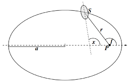
Figure 1: The geometry of the spin–orbit problem: orbital radius $r$, semi-major axis $a$, true anomaly $f$, rotation angle $x$.

Remark 1

• The parameter $\varepsilon={3\over 2}{{I_{2}-I_{1}}\over I_{3}}$ plays the role of the perturbing parameter: the Hamiltonian (1) is integrable whenever $\varepsilon=0$, which corresponds to the equatorial symmetry $I_{1}=I_{2}$. For almost spherical bodies, like the Moon or Mercury, the value of $\varepsilon$ is of the order of $10^{-4}$.

• It is important to stress that (1) is a non–autonomous Hamiltonian function, due to the fact that $r$ and $f$ are Keplerian functions of the time. Introducing the eccentric anomaly $u$, defined in terms of the mean anomaly $\ell_{0}$ (which is a linear function of time) through the well–known Kepler’s equation $\ell_{0}=u-e\sin u$, the orbital radius and the true anomaly can be determined by means of the following Keplerian expressions:

  $$r = a(1-e\cos u)$$

  $$f = 2\arctan\Big{(}\sqrt{{1+e}\over{1-e}}\tan{u\over 2}\Big{)}\ .$$ (3)

• The Hamiltonian (1) depends parametrically on the orbital eccentricity $e$ through $r$ and $f$ provided by (b)). We remark that in the case of circular orbits, equation (2) becomes integrable, since $r$ is constant and $f$ coincides with time (up to a shift).

Expanding $r$ and $f$ given in (b)) in power series of $e$, the Fourier expansion of equation (2) can be written as

$$\ddot{x}\ +\ \varepsilon\ \sum\limits_{m\not=0,m=-\infty}^{+\infty}\ W({m\over 2},e)\ \sin(2x-mt)\ =\ 0\ ,$$ (4)

where we introduced the coefficients $W({m\over 2},e)$, decaying as powers of $e$ (see, e.g., [5]). Using a compact notation, we write (4) as

$$\ddot{x}+\varepsilon V_{x}(x,t)=0\ ,$$ (5)

where $V=V(x,t)$ is a time–dependent periodic function (the subscript $x$ denotes derivative with respect to the argument). In particular, we consider a trigonometric function by retaining in (5) just the most important harmonics (see [5]). Precisely, keeping the same notation $V$ for the trigonometric approximation, we define

$$V(x,t) \equiv -\bigg{[}\big{(}\frac{1}{2}-\frac{5}{4}e^{2}+\frac{13}{32}e^{4}\big{)}\cos(2x-2t)$$ (6)

$$+\big{(}\frac{7}{4}e-\frac{123}{32}e^{3}\big{)}\cos(2x-3t)+\big{(}\frac{17}{4}e^{2}-\frac{115}{12}e^{4}\big{)}\cos(2x-4t)\bigg{]}\ .$$

We now introduce the definition of a $p:q$ spin–orbit resonance for $p,q\in{\mathbb{Z}}$ with $q>0$ as a periodic solution of (4), say $t\in{\mathbb{R}}\to x=x(t)\in{\mathbb{R}}$, such that it satisfies

$$x(t+2\pi q)=x(t)+2\pi p\qquad{\rm for\ any\ }\ t\in\mathbb{R}\ .$$

The above expression implies that the ratio between the period of revolution and the period of rotation is equal to $p/q$. It is widely known that the Moon, alike most of the evolved satellites of the Solar system, move in a 1:1 spin–orbit resonance (usually referred to as the synchronous resonance); within the Solar system only Mercury moves in a non–synchronous resonance ([10], [12]), precisely in a 3:2 spin–orbit resonance, since twice the orbital period is equal to thrice the rotational period within an error of the order of $10^{-4}$ (see [5]).

2.2 The dissipative spin–orbit problem

Due to assumption $iv)$ of Section 2.1, dissipative effects have been discarded and in particular we neglected the effect of the non–rigidity of the satellite. This contribution, which turns out to be the most relevant dissipative effect, induces a tidal torque ([21], [23]), which can be written as a function ${\mathcal{T}}$ depending linearly on the angular velocity $\dot{x}$:

$${\mathcal{T}}(\dot{x};t)=-K_{d}\Big{[}L(e,t)\dot{x}-N(e,t)\Big{]}\ .$$ (7)

In the above expression we have introduced the functions $L$ and $N$ as

$$L(e,t)={a^{6}\over r^{6}}\ ,\qquad N(e,t)={a^{6}\over r^{6}}\dot{f}$$

(recall that $r$ and $f$ are known functions of the time). Moreover, the coefficient $K_{d}$ is the dissipative constant, whose explicit expression is given by

$$K_{d}\equiv 3n\ {{k_{2}}\over{\xi Q}}({R_{e}\over a})^{3}{M\over m}\ ,$$

where $n$ denotes the mean motion (that we have normalized to one), $k_{2}$ is the so–called Love number (see [17]), the constant $\xi$ is defined through $I_{3}=\xi mR_{e}^{2}$ with $R_{e}$ denoting the equatorial radius, $Q$ is called the quality factor (providing the frequency of oscillation with respect to the rate of dissipation of energy, [17]). In order to compare the size of the dissipative effect with that of the conservative part, we notice that astronomical measurements provide a value for $K_{d}$ of the order of $10^{-8}$ for the Moon or Mercury.

In the following we reduce the tidal torque by considering (as in [11]) its average over one orbital period. In particular, taking the average of (7) with respect to time one obtains (see [23])

$$\bar{\mathcal{T}}\equiv\bar{\mathcal{T}}(\dot{x})=-K_{d}\Big{[}\bar{L}(e)\dot{x}-\bar{N}(e)\Big{]}$$ (8)

with

$$\bar{L}(e) \equiv {1\over{(1-e^{2})^{9/2}}}\ (1+3e^{2}+{3\over 8}e^{4})$$

$$\bar{N}(e) \equiv {1\over{(1-e^{2})^{6}}}\ (1+{{15}\over 2}e^{2}+{{45}\over 8}e^{4}+{5\over{16}}e^{6})\ .$$ (9)

In conclusion, the following differential equation describes the spin–orbit problem under the dissipative effect due to the tidal torque:

$$\ddot{x}\ +\varepsilon\Big{(}{a\over r}\Big{)}^{3}\ \sin(2x-2f)=-K_{d}\Big{[}\bar{L}(e)\dot{x}-\bar{N}(e)\Big{]}\ .$$ (10)

As in (5), we use a compact notation re-writing (10) as

$$\ddot{x}\ +\varepsilon V_{x}(x,t)=-\mu(\dot{x}-\eta)\ ,$$ (11)

where we have introduced $\mu$ and $\eta$ as follows: $\mu\equiv K_{d}\bar{L}(e)$, $\eta\equiv\bar{N}(e)/\bar{L}(e)$. As we can see, $\mu$ depends on the dissipative constant (as well as on $e$), and therefore we call it dissipative parameter, while $\eta$ is just a function of the eccentricity, and we call it the drift parameter.

Remark 2

The tidal torque in (11) vanishes for $\dot{x}=\eta$; in view of (8), the tidal torque vanishes as far as

$$\dot{x}\equiv{{\bar{N}(e)}\over{\bar{L}(e)}}={{1+{15\over 2}e^{2}+{45\over 8}e^{4}+{5\over{16}}e^{6}}\over{(1-e^{2})^{3\over 2}(1+3e^{2}+{3\over 8}e^{4})}}\ .$$ (12)

When $e=0$ equation (12) implies that $\dot{x}=1$, which corresponds to the synchronous resonance. For the actual Mercury’s eccentricity amounting to $e=0.2056$, (12) provides the value $\dot{x}=1.256$, while for future use we notice that $e=0.285$ corresponds to $\dot{x}=1.5$, namely the 3:2 resonance.

3 A normal form construction

Our next task is to develop a normal form which transforms (11) into a system of equations which is normalized up to a given order (see [8]). This allows us to compute a normalized frequency, which will provide useful information on the dynamical behavior of the model described by (11).

Let us write (11) as the first–order differential system

$$\dot{x} = y$$

$$\dot{y} = -\varepsilon V_{x}(x,t)-\mu(y-\eta)\ .$$ (13)

Let us denote the frequency vector of motion associated to the one–dimensional, time dependent equation (3) as $\omega(y)=(\omega_{0}(y),1)$. Assume that the vector field (3) is defined on a set $A\times{\mathbb{T}}^{2}$, where $A\subset\mathbb{R}$ is an open set. Let $y_{0}\in A$ be an initial condition such that the frequency $\omega_{0}=\omega_{0}(y_{0})$ satisfies the following non–resonance condition:

$$|\omega_{0}m+n|>0\qquad{\rm for\ any}\ \ (m,n)\in{\mathbb{Z}}^{2}\ ,\quad n\not=0\ .$$

We look for a transformation of coordinates defined up to a suitable order $N\in{\mathbb{Z}}_{+}$ in $\varepsilon,\mu$, say $\Xi_{N}:A\times{{\mathbb{T}}}^{2}\rightarrow{\mathbb{R}}\times{{\mathbb{T}}}^{2}$, such that the new variables are $(Y,X)$ with

$$(Y,X,t)=\Xi_{N}(y,x,t)\ ,\qquad Y\in{\mathbb{R}}\ ,\quad(X,t)\in{{\mathbb{T}}}^{2}\ .$$ (14)

In the transformed set of coordinates we require that the equations become:

$$\dot{X} = \Omega(Y;\varepsilon)+O_{N+1}(\varepsilon,\mu)$$

$$\dot{Y} = -\mu(Y-\eta)+O_{N+1}(\varepsilon,\mu)\ ,$$ (15)

where $O_{N+1}(\varepsilon,\mu)$ denotes a function whose Taylor series expansion in $\varepsilon$, $\mu$ contains only monomials $\varepsilon^{j}\mu^{m}$ with $j+m\geq N+1$.

According to [8], the transformation (14) is obtained as the composition of two transformations. The first one brings the original variables $(x,y,t)$ into intermediate variables $(\tilde{x},\tilde{y},t)$, so to remove terms depending on $\varepsilon$; then, from $(\tilde{x},\tilde{y},t)$ we implement another change of variables to $(X,Y,t)$ in such a way to obtain (3).

The normal form (3) is particularly useful, since neglecting $O_{N+1}(\varepsilon,\mu)$ one can integrate the second equation as

$$Y(t)=\eta+(Y_{0}-\eta)\ e^{-\mu(t-t_{0})}\ ,$$ (16)

where we denote by $(X_{0},Y_{0})$ the initial conditions at time $t=t_{0}$ in the normal form variables. The expression (16) shows that, in the approximation obtained neglecting higher order terms, the solution tends to $Y=\eta$ as time tends to infinity. Inserting (16) into the first of (3) we obtain the dependence of $\dot{X}$ on time, whose integration provides $X=X(t)$ with $X(0)=X_{0}$. Indeed the solution (16) provides the natural attractor, which can be found in the original coordinates by integrating equations (3) with $\varepsilon=0$.

The local behavior near quasi–periodic attractors of some dissipative systems, precisely conformally symplectic systems, has been studied in [4]. The main result of [4] is that there exists a transformation of coordinates such that the time evolution becomes a rotation in the angles and a contraction in the actions. The normal form (3) is consistent with such result: indeed, neglecting higher order terms, the expression (16) shows that the normalized action contracts exponentially in the dissipative parameter, while the first of (3) shows that the limiting behavior of the normalized angle is a linear rotation with frequency $\Omega(\eta)$.

For details on the normal form algorithm used to obtain (3) we refer to [8]; here we just state the final result. At the normalization order $N=3$ the normalized frequency $\Omega(Y;\varepsilon)$ in (3) turns out to be

$$\Omega(Y;\varepsilon) = Y-\frac{\varepsilon^{2}}{8(Y-1)^{3}}+\varepsilon^{2}\bigg{[}\frac{1}{8}e^{2}\left(\frac{5}{(Y-1)^{3}}+\frac{98}{(3-2Y)^{3}}\right)+$$

$$\frac{1}{64}e^{4}\left(-\frac{63}{(Y-1)^{3}}+\frac{3444}{(2Y-3)^{3}}-\frac{578}{(Y-2)^{3}}\right)+$$

$$\frac{1}{768}e^{6}\left(\frac{31280}{(Y-2)^{3}}+\frac{390}{(Y-1)^{3}}+\frac{45387}{(3-2Y)^{3}}\right)\bigg{]}\ ,$$

where we expanded the coefficients up to the 6th order in the eccentricity. The expansion of the drift $\eta=\bar{N}(e)/\bar{L}(e)$ (with $\bar{N}$, $\bar{L}$ as in (2.2)) to the same order is given by:

$$\eta=1+6e^{2}+\frac{3e^{4}}{8}+\frac{173e^{6}}{8}\ .$$ (18)

Equations (3) together with (3), (18) will be used in Section 5.2 for a dynamical investigation based on a normal form approach; precisely, we will backtransform the frequency $\Omega$ in the original variables and compare the result with a numerical integration.

4 A parametric representation of invariant attractors

With reference to equation (11), we introduce in this Section a parametric representation of an invariant KAM attractor with Diophantine frequency; as it is well known ([3], [6]), the equations for the embedding can be solved under suitable compatibility conditions, which provide a relation between the frequency and the drift. In particular, such compatibility conditions allow us to provide an explicit computation of the drift that we perform up to the 4-th order in the series development in the perturbing parameter. These results are used in Section 5.3 in order to investigate in some specific cases the relation between the drift and the frequency, as well as the dependence on the other parameters (most notably the oblateness and the eccentricity).

Let us recall that the frequency vector of motion associated to (11) is written as $\omega=(\omega_{0},1)$. We say that $\omega$ satisfies the Diophantine condition, whenever the inequality

$$|\omega_{0}\ m+n|^{-1}\ \leq\ C|m|\qquad{\rm for\ all}\ \ (m,n)\in{\mathbb{Z}}^{2}\ ,\quad m\not=0$$ (19)

is satisfied for some positive real constant $C$. Next we provide the following definition of a KAM attractor for (11).

Definition 3

A KAM attractor for (11) with rotation number $\omega=(\omega_{0},1)$ satisfying (19) is a two–dimensional invariant surface, described parametrically by

$$x=\theta+u(\theta,t)\ ,\quad(\theta,t)\in{\mathbb{T}}^{2}\ ,$$ (20)

where the flow in the parametric coordinate is linear, namely $\dot{\theta}=\omega_{0}$, and where $u=u(\theta,t)$ is a suitable analytic, periodic function, such that

$$1+u_{\theta}(\theta,t)\not=0\quad{\rm for\ all}\ (\theta,t)\in{\mathbb{T}}^{2}\ .$$ (21)

Let $D$ be the partial derivative operator defined as

$$D\equiv\omega_{0}{\partial\over{\partial\theta}}+{\partial\over{\partial t}}\ .$$ (22)

Inserting (20) in (11) and using the definition (22), it is readily seen that the function $u$ must satisfy the differential equation

$$D^{2}u(\theta,t)+\varepsilon V_{x}(\theta+u(\theta,t),t)=-\mu\Big{(}\omega_{0}+Du(\theta,t)-\eta\Big{)}\ .$$ (23)

Notice that the inversion of the operator $D^{2}$ provokes the appearance of the well–known problem of the small divisors ([5]). An approximate solution of (23) can be found as follows. Let us expand $u$ and $\eta$ in Taylor series of $\varepsilon$ as

$$u(\theta,t)=\sum_{k=1}^{\infty}u_{k}(\theta,t)\varepsilon^{k}\ ,\qquad\eta=\sum_{k=0}^{\infty}\eta_{k}\varepsilon^{k}\ .$$ (24)

Inserting (24) in (23) and equating same orders in $\varepsilon$, one obtains the iterative equations

$$D^{2}u_{1}(\theta,t)+\mu Du_{1}(\theta,t) = -V_{x}(\theta,t)+\mu\eta_{1}$$

$$D^{2}u_{2}(\theta,t)+\mu Du_{2}(\theta,t) = -V_{xx}(\theta,t)\ u_{1}(\theta,t)+\mu\eta_{2}$$

$$...$$

$$D^{2}u_{k}(\theta,t)+\mu Du_{k}(\theta,t) = S_{k}(\theta,t)+\mu\eta_{k}\ ,$$ (25)

where at the order $k$ the function $S_{k}$ is known and it depends on the derivatives of $V$ as well as on $u_{1}$, …, $u_{k-1}$. At each order one determines first $\eta_{k}$ so that the right hand sides of (4) have zero average. After having determined $\eta_{k}$, the $k$–th equation in (4) can be used to find $u_{k}$ as the solution of the following equation:

$$D^{2}u_{k}(\theta,t)+\mu Du_{k}(\theta,t)=\widetilde{S}_{k}(\theta,t)\ ,$$ (26)

where $\widetilde{S}_{k}$ has zero average (in fact, $\widetilde{S}_{k}=S_{k}-\bar{S}_{k}$, where the bar denotes the average over $\theta$ and $t$). To solve (26), let us expand $u_{k}$ in Fourier series as

$$u_{k}(\theta,t)=\sum_{(m,n)\in{\mathbb{Z}}^{2}}\hat{u}_{mn}^{(k)}\ e^{i(m\theta+nt)}\ ,$$

where $\hat{u}_{mn}^{(k)}$ denote the (unknown) Fourier coefficients of $u_{k}$. Inserting the Fourier series in (26) and expanding also the left hand side in Fourier series, we obtain

$$\sum_{(m,n)\in{\mathbb{Z}}^{2}}\Big{[}-(\omega_{0}m+n)^{2}+i\mu(\omega_{0}m+n)\Big{]}\ \hat{u}_{mn}^{(k)}\ e^{i(m\theta+nt)}=\sum_{(m,n)\in{\mathcal{I}}_{S}^{(k)}}\hat{S}_{mn}^{(k)}\ e^{i(m\theta+nt)}\ ,$$ (27)

where ${\mathcal{I}}_{S}^{(k)}$ denotes the set of the Fourier indexes of $\widetilde{S}_{k}$. Equation (27) allows to determine $u_{k}$ as

$$u_{k}(\theta,t)=\sum_{(m,n)\in{\mathcal{I}}_{S}^{(k)}}{{\hat{S}_{mn}^{(k)}}\over{-(\omega_{0}m+n)^{2}+i\mu(\omega_{0}m+n)}}\ e^{i(m\theta+nt)}\ .$$ (28)

Notice that the assumption (19) on $\omega_{0}$ guarantees that $u_{k}$ is well defined (no zero divisors appear in (28)). An alternative (weaker) assumption would be that $|\omega_{0}m+n|>0$ for all $(m,n)\in{\mathcal{I}}_{S}^{(k)}$.

Due to the fact that the function $V$ is assumed to be a trigonometric function (see (6)), also $S_{k}$ is trigonometric and it is convenient to write it as

$$S_{k}(\theta,t)=\sum_{(m,n)\in{\mathcal{I}}_{S}^{(k)}}\Big{[}\hat{S}_{mn}^{(k,c)}\cos(m\theta+nt)+\hat{S}_{mn}^{(k,s)}\sin(m\theta+nt)\Big{]}$$

for suitable real coefficients $\hat{S}_{mn}^{(k,c)}$ and $\hat{S}_{mn}^{(k,s)}$. Then in place of (26) we can write the solution in a real form which is suitable for numerical computations as

$$u_{k}(\theta,t) = -\sum_{m,n\in{\mathcal{I}}_{S}}\Big{[}{{\hat{S}_{mn}^{(k,c)}}\over{(\omega_{0}m+n)[(\omega_{0}m+n)^{2}+\mu^{2}]}}\ \Big{(}(\omega_{0}m+n)\cos(m\theta+nt)-\mu\sin(m\theta+nt)\Big{)}$$

$$+ {{\hat{S}_{mn}^{(k,s)}}\over{(\omega_{0}m+n)[(\omega_{0}m+n)^{2}+\mu^{2}]}}\ \Big{(}(\omega_{0}m+n)\sin(m\theta+nt)+\mu\cos(m\theta+nt)\Big{)}\Big{]}\ .$$

In conclusion, the algorithm to compute the drift consists in solving iteratively equations (4) to obtain the functions $u_{k}$; at each order, by imposing that the right hand sides have zero average, we obtain the terms $\eta_{k}$ of the series expansion (24) of the drift.

We provide here the $\eta_{k}$ expanded up to the third order (the fourth order can be obtained through a reasonable computer time, but the expression becomes too long to be displayed here):

$$\eta_{0} = \omega_{0}$$

$$\eta_{1} = \eta_{3}=0$$

$$\eta_{2} = -\frac{a^{2}}{2(\omega-1)\left(\mu^{2}+4(\omega-1)^{2}\right)}-\frac{b^{2}}{(2\omega-3)\left(\mu^{2}+(3-2\omega)^{2}\right)}$$ (29)

$$- \frac{c^{2}}{(2\omega-1)\left(\mu^{2}+4(1-2\omega)^{2}\right)}$$

with

$$a=1-\frac{5e^{2}}{2}+\frac{13e^{4}}{16}\ ,\qquad b=\frac{7e}{2}-\frac{123e^{3}}{16}\ ,\qquad c=-\frac{1}{6}e^{2}\left(115e^{2}-51\right)\ .$$

The above solution for $\eta$ defines the drift parameter in (24) up to finite order; this expression will be used in Section 5.3 to obtain in particular a constraint between the parameters of the model (precisely, the oblateness parameter and the eccentricity).

5 Transient time and attractor’s drift

We devote this Section to the discussion of some dynamical features of the attractors associated to the model described by equation (11). In particular, we provide a numerical method (see Section 5.1) which allows to determine the time needed to reach an attractor. Indeed, the computation of such transient time is a critical issue in the study of dissipative systems. Next, we make a comparison between the results obtained through the normal form computation of Section 3 as well as those provided by the parametrization in Section 4 with the results obtained from direct numerical simulations (see Section 5.2). A link between the oblateness parameter and the eccentricity is provided in Section 5.3 as a consequence of the construction of the drift term through the parametric representation of Section 4.

5.1 A numerical investigation of the transient time

The numerical determination of the frequency of an attractor is usually a cumbersome problem, since the time necessary to reach an attractor is often strongly influenced by the strength of the dissipation. With reference to (11), if $\mu$ is small, then one typically needs to wait for a longer time to be on the attractor, while for $\mu$ large, the transient time is shorter. There is an intrinsic difficulty to measure the time to reach the attractor and of course this might affect also the computation of the frequency. In principle, Lyapunov exponents can be used to compute the transient time by evaluating the moment at which they reach convergence. It should be remarked that Lyapunov exponents provide more indications on the dynamics, precisely on the rate growth of the phase space volume. Notwithstanding these remarks, we present an alternative numerical recipe which provides information on the attractor’s frequency. It turns out, that the computer execution time becomes longer with respect to the computation based on our method (about a factor 2).

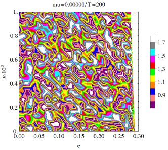
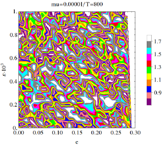
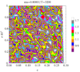
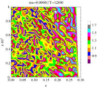
Figure 2: The value $\omega_{num}$ in the space $(e,\varepsilon)$ for $\mu=10^{-5}$ and integration times $T=200,800,3200,12800$. The colors show the values of the frequency as given in the column bar.

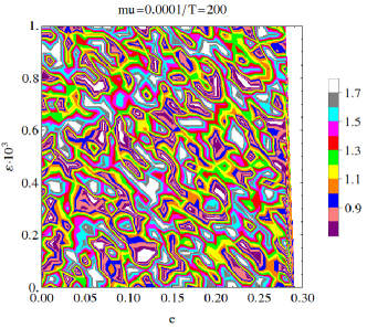
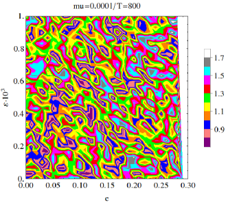
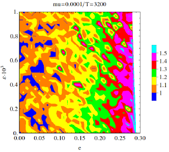
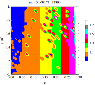
Figure 3: The value $\omega_{num}$ in the space $(e,\varepsilon)$ for $\mu=10^{-4}$ and different integration times $T=200,800,3200,12800$. The colors show the values of the frequency as given in the column bar.

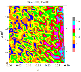
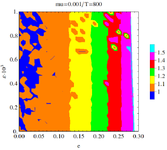
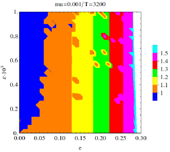
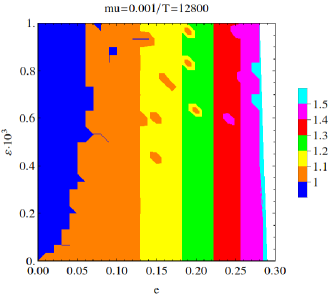
Figure 4: The value $\omega_{num}$ in the space $(e,\varepsilon)$ for $\mu=10^{-3}$ and different integration times $T=200,800,3200,12800$. The colors show the values of the frequency as given in the column bar.

First, we integrate the original equations of motion (3) with $V$ given in (6) in the parameter space $\mu\times\varepsilon\times e$ for fixed $\mu$ (e.g. $\mu=10^{-3},10^{-4},10^{-5}$), on a finite grid (e.g. $30\times 30$ values) in given intervals of $\varepsilon$, $e$ (e.g. $0\leq\varepsilon\leq 10^{-3}$, $0\leq e\leq 0.3$). The value of the drift has been computed as a function of the eccentricity as $\eta=\bar{N}(e)/\bar{L}(e)$. We use different integration times $t_{T}=2\pi T$ with $T=100,200,400,\ldots,12800$ (the last value is taken in order to obtain results within a reasonable computer time).

Our choice of the parameters is made to cover the regime of interest for physical applications. The upper bound 0.3 on the eccentricity encompasses both the eccentricity of Mercury, about equal to 0.2, which is the largest body in a spin–orbit resonance, and it is bigger than the value 0.285 which corresponds to the 3:2 resonance (see Remark 2). Moreover, typical values for $\varepsilon$ are $10^{-4}$ for the Moon or Mercury, $10^{-3}$ or even larger for the irregular satellites of our solar system. Using $e\sim 0.3$, $\varepsilon\sim\mu\sim 10^{-3}$, a third order normal form gives an error, e.g. in (17), of about $10^{-12}$, which is well below the numerical error that we introduced in our numerical studies.

Let $\{x_{k},y_{k}\}$ be an orbit computed at times multiple of $2\pi$, namely $x_{k}=x(2\pi k)$, $y_{k}=y(2\pi k)$ with $k=1,\ldots,T$. We are interested in the limiting behavior of the frequency $\omega_{k}=\omega\left(y_{k}\right)$ as $k$ approaches $T$. Let us focus on the value of the frequency when approaching the maximum time $T$, say $k=9/10T,\ldots,T$. From the expression

$$\omega_{num}=\frac{10}{T}\sum_{k=9/10T}^{T}\omega_{k}\ ,$$

we are able to estimate the mean value of $\left\{\omega_{k}\right\}$ in the proximity of $T$, taking the first part of the orbit as transient. Next step consists in finding a linear model of the form $\omega_{k}=\omega_{num}+\sigma k$ through $\left\{\omega_{k}\right\}$: the parameter $\sigma$ quantifies the slope in $\left\{\omega_{k}\right\}$. We claim that $\omega_{num}$ is close to the final frequency on the attractor if $\sigma\to 0$. We provide now an example and we add a discussion on $\sigma$ at the end of this Section.

We implement this procedure in a specific case, which is illustrated in Figure 2. We start with a sample where $\omega_{num}$ does not coincide with the final frequency on the attractor. In fact, for $\mu=10^{-5}$ no regular pattern for $\omega_{num}$ can be seen in Figure 2. The dynamics takes place in an intermediate regime, where $\omega_{num}$ still suffers huge variations in time. In this example, the slope $\sigma$ is still of the order of $10^{-3}$ for $T=100$ and $10^{-5}$ for $T=12800$. After an integration time long enough, at $T=12800$ we start observing some structures, since $\omega_{num}=1$ accumulates for small $e$, while $\omega_{num}=1.5$ is obtained for larger values of the eccentricity. This behavior would be more evident for longer integration times and it will occur for a larger value of the dissipative parameter (see Figures 3 and 4). The conclusion is that for this set of parameters a longer time is necessary to obtain that the dynamics has reached the attractor. If we increase the dissipative parameter, we obtain better results on the above time scales. In fact, for $\mu=10^{-4}$ we find (see Figures 3 and 5) that $\sigma$ runs from $10^{-3}$ for $T=100$ to $10^{-6}$ for $T=12800$. Therefore, increasing $\mu$ by one order of magnitude the slope $\sigma$ decreases by one order at $T=12800$. For integration times long enough, we also clearly see that we get a frequency $\omega_{num}$ which is almost constant for a fixed value of the eccentricity as $\varepsilon$ varies.

When we increase further the strength of the dissipation, we see that the attractor is reached on a shorter time scale. Indeed, for $\mu=10^{-3}$ the slope $\sigma$ ranges from $10^{-3}$ for $T=100$ to $10^{-7}$ for $T=12800$. Again we see a very clear separation of $\omega_{num}$ at fixed values of $e$, and that the dependency of $\omega_{num}$ on $\varepsilon$ is small (see Figure 4).

It is possible to quantify the level of accuracy of our numerical approach by investigating the size of $\sigma$ and its dependency on the integration time. In Figure 5 we provide the absolute value of $\sigma$ versus the integration time $T$ that we increased up to $T=102400$ to be able to see also the limiting behaviour for all values of the parameters, including $\mu=10^{-5}$. We clearly see that the larger the value of $\mu$ or the longer the integration times $T$, the smaller the value of $\sigma$. Such behavior of $\sigma$ provides a strong indication on the transient time to reach the attractor.

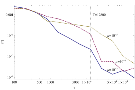
Figure 5: The maximal absolute value of $\sigma$ versus the integration time $T$ for different values of the dissipative parameter $\mu$. The larger $\mu$ or the longer the integration time $T$, the smaller the linear drift $|\sigma|$ (we increased $T$ for these specific cases to reach the error of the numerical integration scheme, that also explains the fluctuations of $\sigma$ close to $10^{-8}$).

5.2 Using the normal form approach

We proceed to compute the normalized frequency, that we can obtain by implementing the normal form described in Section 3. Precisely, we use the solution for the normalized frequency (3), where (with a little abuse) we replace $Y$ by its limiting value $Y_{\infty}=\eta$. The drift $\eta$ is expanded up to finite order in the eccentricity as in (18). This yields a good approximation of the normalized frequency that we call $\Omega_{app}=\Omega_{app}(\varepsilon,e)$ . The analytical result will be compared with the frequency $\omega_{num}$, that we obtained from the numerical simulations described in Section 5.1.

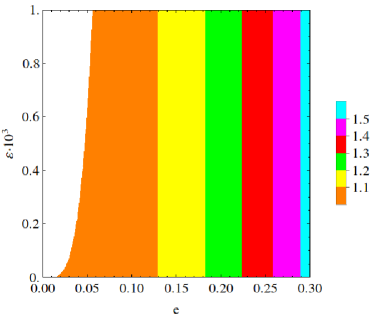
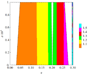
Figure 6: Frequencies $\Omega_{app}$ and $\omega_{app}(y(Y_{\infty},X_{\infty};\varepsilon,\mu))$ in the parameter space $(e,\varepsilon)$ obtained from the normal form approach: normalized frequency (left), back-transformed frequency (right) with $\mu=10^{-3}$. The figures have to be compared with the panels of Figure 4.

In Figure 6 (left) we show the frequency $\Omega_{app}$ obtained from the normal form equation in the plane $(\varepsilon,e)$. By comparing Figure 6 with Figures 2– 4, one can see that the frequencies calculated using the normal form coordinates are in good agreement with the frequencies that we obtain from the numerical approach. We also report the frequency that we calculated in the normalized variables in terms of the original variables. To this end we need to compute the inverse of the transformation $\Xi_{N}(y,x,t;\varepsilon,\mu)$ in (14), say $\Xi_{N}^{-1}(Y,X,t;\varepsilon,\mu)$, replace for $X,Y$ the limits $X_{\infty},Y_{\infty}$, and calculate the average over time to get $\omega_{app}(y(Y_{\infty},X_{\infty};\varepsilon,\mu))$. The results concerning the normalized frequency in the original variables are given in Figure 6 (right); the values of Figure 6 (right) and those of Figure 4 (last panel) perfectly agree in the non-resonant regime, while close to the main resonances corresponding to the white empty zones (precisely, 1:1, 5:4, 3:2 resonances, corresponding to the outermost left zone close to $e=0$, the tongue originating at $e=0.2$ and the right white zone at about $e=0.29$), the non-resonant normal form together with the transformation cannot be used, due to the accumulation of zero divisors in the denominators of the analytic expansions. Note that in Figure 6 (left) the plot is independent of $\mu$, since $\Omega_{app}=\Omega_{app}(\varepsilon,e)$, see (3), turns out to be independent of $\mu$, while there is a parametric dependency of $\omega_{app}$ on $\mu$ due to the fact that we used the inverse transformation $\Xi_{N}^{-1}(X,Y,t;\varepsilon,\mu)$.

5.3 A constraint resulting from the parametrization

In the previous sections we concentrated on the computation of the frequency of motion for given values of the parameters, including the drift parameter. Nevertheless, in many physical situations we might be interested to focus on a specific frequency; however, fixing the frequency means that we need to find the drift parameter in terms of such frequency as well as $\varepsilon$, $e$. This can be done in the case of non–resonant frequencies by implementing the parametric representation of invariant tori described in Section 4. Indeed, in order to be able to solve the equations (4) we must compute the terms $\eta_{k}$ of the series expansion of $\eta$ in (24) as given by the expressions (4), say $\eta=\eta(\omega,e,\varepsilon,\mu)$. Normally the procedure is to fix $\varepsilon,\mu$ and to find a relation between the drift $\eta$ and the frequency. Given that $\eta$ is a function of the eccentricity, this procedure amounts to producing a relation between the eccentricity and the frequency for fixed values of $\eta,\mu$. However, we can decide to fix the frequency $\omega$ and to let $\varepsilon$ vary in order to obtain an expression between the eccentricity $e$ and the shape parameter $\varepsilon$.

More precisely, the quantity $\eta$, itself, is given as a function of the eccentricity $e$ through $\eta=\bar{N}(e)/\bar{L}(e)$, as we can notice from the original equation of motion (11). Therefore, we are led to introduce the function

$$C(\omega,e,\varepsilon,\mu)\equiv\bar{N}(e)/\bar{L}(e)-\eta(\omega,e,\varepsilon,\mu)$$ (30)

and we look for contour plots of $C(\omega,e,\varepsilon,\mu)$ in the space $e\times\varepsilon$ for fixed values of $\omega$, $\mu$. To avoid zero divisor evaluations we replace $\omega$ with irrational frequencies $\omega_{k}$ obtained through the formula

$$\omega_{k}=\frac{p}{q}\pm\frac{1}{k+\gamma}\ ,$$

where $p/q$ denotes the exact resonant value, $\gamma=(\sqrt{5}-1)/2$, and $k=50,60,70,80,90,100$. We show the results for the $2:1$, $3:2$, $4:3$, and $1:1$ resonance in Figure 7. For the 1:1 resonance we can compute the approximations only from above (namely $\omega_{k}=1+\frac{1}{k+\gamma}$), since the rotational history of the satellites allows to state that celestial bodies rotated fast in the past and that they slowed down due to the dissipation, eventually ending their evolution in a 1:1 resonance, which corresponds to circular orbits in the case of vanishing tidal torque (see Remark 2). In Figure 7 the dissipative parameter is fixed to $\mu=10^{-3}$ and $\varepsilon$ versus $e$ is shown. Since the eccentricity is related to the drift parameter through $\eta=\bar{N}(e)/\bar{L}(e)$, the above picture is essentially equivalent to showing the perturbing versus the drift parameter.

As Figure 7 shows, using equation (30), which depends on the computation of the parametrization of the invariant attractor, we are able to relate the shape parameter $\varepsilon$ of the rotating body with the orbital parameter $e$, thus providing an interesting information from the astronomical point of view. On the other hand, though typically periodic orbits are used to approximate invariant tori (just taking the rational approximants to the irrational - Diophantine - frequency), Figure 7 provides an indication of how the invariant KAM tori approximate the main resonances ($2:1$, $3:2$, $4:3$, $1:1$). In Figure 7 we observe the accumulation of straight lines, which are parallel to the dashed lines that indicate the exact positions of the $p/q=4:3$ and $p/q=2:1$ resonances. Though not being possible to distinguish the separate lines graphically in Figure 7, we confirm that the curves defined by $C=0$ tend to the dashed curves defined by $\eta(e)=p/q$ for larger $k$, and arbitrary $\varepsilon$. On the contrary, for the $1:1$ and $3:2$ resonances we observe that the curves start to converge to the dashed lines for small $\varepsilon$, while they bend for $\varepsilon$ larger. We believe that a higher order expansion should be computed for larger values of the perturbing parameters, since getting closer to the resonances the effect of the small divisors becomes amplified, thus leading to the divergence of the series defining the parametrization.

The $1:1$ resonance is very common for several natural satellites in the solar system. A future study of the $1:1$ resonance may provide further information. Beside that, we think that our relation provides an interesting information concerning how the oblateness parameter is linked to the eccentricity in the proximity of the different kinds of resonances.

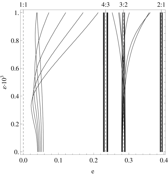
Figure 7: Contours obtained from the relation $C(\omega,e,\varepsilon,\mu)$ for different $\omega_{k}={p\over q}\pm{1\over{k+\gamma}}$ ($\gamma$ being the golden ratio) with $k=50,\dots,100$, and $\mu=10^{-3}$ in the space $e\times\varepsilon$ for $\omega_{k}$ close to the following $p:q$ resonances: $2:1$, $3:2$, $4:3$, $1:1$.

6 Conclusions

We have investigated some dynamical features of the dissipative spin–orbit problem, modeling the dynamics of a non–rigid satellite orbiting on a Keplerian ellipse around a central planet. In particular we have focused on the transient time to reach an attractor; this transient time is often decided on the basis of numerical experiments, integrating the vector field on longer time scales and looking for the convergence of some quantities providing an indication that the attractor is reached. Here we have proposed a method which is based on the analytical development of a dissipative normal form. This construction allows to compare the normalized frequency with that obtained integrating the original equations on longer time scales. The normal form, suitably developed to parametrize invariant attractors, provides also an explicit expression of the drift term for a specific attractor with fixed frequency. This allows to give a constraint between the oblateness parameter and the eccentricity, which may be particularly relevant in astronomical applications.

Acknowledgements. A.C. was partially supported by PRIN-MIUR 2010JJ4KPA$\_$009, GNFM-INdAM and by the European MC-ITNs Astronet-II and Stardust. C.L. was partially supported by the ESA-BELSPO grant Prodex C90253 and the Austrian Science Fund (FWF): J3206.

References

- [1] H.W. Broer, G.B. Huitema, M.B. Sevryuk, Quasi–periodic motions in families of Dynamical systems, Lecture Notes in Mathematics 1645, Springer–Verlag (1996)
- [2] H.W. Broer, C. Simó, J.C. Tatjer, Towards global models near homoclinic tangencies of dissipative diffeomorphisms, Nonlinearity 11, no. 3, 667–770 (1998)
- [3] R. Calleja, A. Celletti, R. de la Llave, A KAM theory for conformally symplectic systems: efficient algorithms and their validation, J. Differential Equations 255, n. 5, 978–1049 (2013)
- [4] R. Calleja, A. Celletti, R. de la Llave, Local behavior near quasi-periodic solutions of conformally symplectic systems, J. Dynam. Differential Equations 25, n. 3, 978–1049 (2013)
- [5] A. Celletti, Stability and Chaos in Celestial Mechanics, Springer-Verlag, Berlin; published in association with Praxis Publishing Ltd., Chichester, ISBN: 978-3-540-85145-5 (2010)
- [6] A. Celletti, L. Chierchia, Quasi-periodic attractors in Celestial Mechanics, Archive for Rational Mechanics and Analysis 191, no. 2, 311–345 (2009)
- [7] A. Celletti, C. Froeschlé, E. Lega, Dynamics of the conservative and dissipative spin–orbit problem, Planetary and Space Science 55, 889–899 (2007)
- [8] A. Celletti, C. Lhotka, Normal form construction for nearly-integrable systems with dissipation, Regular and Chaotic Dynamics 17, n. 3–4, 273–292 (2012)
- [9] M.-C. Ciocci, A. Litvak-Hinenzon, H.W. Broer, Survey on dissipative KAM theory including quasi-periodic bifurcation theory. London Math. Soc., Lecture Notes Ser., 306, Geometric Mechanics and Symmetry. The Peyresq Lectures, 303–355. Cambridge Univ. Press (2005)
- [10] G. Colombo, I.I. Shapiro, The Rotation of the Planet Mercury, Astroph. J. 145, 296–307 (1966)
- [11] A.C.M. Correia, J. Laskar, Mercury’s capture into the 3/2 spin–orbit resonance as a result of its chaotic dynamics, Nature 429, 848–850 (2004)
- [12] A.C.M. Correia, J. Laskar, Mercury’s capture into the 3/2 spin–orbit resonance including the effect of core–mantle friction, Icarus 201, Issue 1, 1–11 (2009)
- [13] A. Delshams, A. Guillamon, J.T. Lazaro, A pseudo-normal form for planar vector fields, Qual. Theory Dyn. Syst. 3, n. 1, 51–82 (2002)
- [14] S. Di Ruzza, C. Lhotka, High order normal form construction near the elliptic orbit of the Sitnikov problem, Celest. Mech. Dyn. Astr. 111, 449–464 (2011)
- [15] A.V. Doroshin, Modeling of chaotic motion of gyrostats in resistant environment on the base of dynamical systems with strange attractors, Comm. Nonlinear Sc. Num. Sim. 16, 3188 -3202 (2011)
- [16] F. Fassò, Lie series method for vector fields and Hamiltonian perturbation theory, J. Appl. Math. Phys. 41 843–864 (1990)
- [17] P. Goldreich, S. Soter, in the Solar System, Icarus 5, 375–389 (1966)
- [18] B.R. Hunt, J.A. Kennedy, T-Y. Li, H.E. Nusse eds., The Theory of Chaotic Attractors, Springer–Verlag, New York (2004)
- [19] H. Kantz, T. Schreiber, Nonlinear Time Series Analysis, Cambridge University Press (1997)
- [20] G. Iooss, E. Lombardi, Polynomial normal forms with exponentially small remainder for analytic vector fields, J. Diff. Eq. 212, 1–61 (2005)
- [21] G.J.F. MacDonald, Tidal friction, Rev. Geophys. 2, 467–541 (1964)
- [22] C.D. Murray, S.F. Dermott, Solar system dynamics, Cambridge University Press (1999)
- [23] S.J. Peale, The free precession and libration of Mercury, Icarus, 178, 4–18 (2005)
- [24] G. Pucacco, D. Boccaletti, C. Belmonte, Periodic orbits in the logarithmic potential, Astronomy & Astrophysics 489, 1055–1063 (2008)