Mapping de Rham-Gabadadze-Tolley bigravity into braneworld setup
Abstract
We discuss whether or not bigravity theory can be embedded into the braneworld setup. As a candidate, we consider Dvali-Gabadadze-Porrati two-brane model with the Goldberger-Wise radion stabilization. We will show that we can construct a ghost free model whose low energy spectrum is composed of a massless graviton and a massive graviton with a small mass. As is expected, the behavior of this effective theory is shown to be identical to de Rham-Gabadadze-Tolley bigravity. Unfortunately, this correspondence breaks down at a relatively low energy due to the limitation of the adopted stabilization mechanism.
I Introduction
Recently, a framework of covariant bimetric gravity with no ghost has been established HR1 . Gravitational theory with two interacting metrics in general suffers from an unwanted ghost degree of freedom, called Boulware-Deser(BD) ghost BD . The finding was that the ghost-free condition is satisfied by assuming a restricted form of interaction between two metrics, which is called de Rham-Gabadadze-Tolley (dRGT) bigravity dRGT1 ; dRGT2 ; HR2 . This interaction has only few parameters and makes one of the two graviton modes massive. In dRGT bigravity, properties of the cosmological and/or black-hole solutions have been already studied cos1 ; cos2 ; cos3 ; cos4 ; cos5 ; BH1 ; BH2 ; GW . However, it is difficult to have physical intuition about these properties. This is partly because the form of interaction between two metrics was technically derived so as to erase the ghost. Furthermore, it is not so clear whether or not this theory can be derived from a more natural setup as a low energy effective theory.
In order to improve our understanding of dRGT bigravity, we consider to reproduce this model in a braneworld setup as a low energy effective theory. Two metrics in dRGT bigravity will be identified with the metrics induced on two branes embedded in higher dimensional bulk spacetime. The toy models with two branes placed in five dimensional bulk have been rather extensively studied RS1 ; RS2 . In order to realize a model that effectively includes only two gravitons, the mass hierarchy between the lowest massive Kaluza-Klein (KK) graviton and the other massive ones will be required. The eigenvalue problem that determines the 4-dimensional mass spectrum in the model with a compact extra dimension is analogous to the eigenvalue problem in quantum mechanics of a particle in one-dimensional potential. In the quantum mechanical problem two small energy eigenvalues can be realized by introducing two deep effective potential wells isolated by a sufficiently high potential barrier. The two lowest energy eigenstates are given by superpositions of the approximate ground states in the respective potential wells: the lowest eigenmode becomes a massless mode and the other mode gains a small mass suppressed by the tunnelling probability between the two potential wells. The energy eigenvalues of the other modes are determined by the typical energy scale of the potential wells, and they are much larger if the potential wells are sufficiently deep or equivalently the barrier between two potential wells is sufficiently high. In this manner, the hierarchy of the energy spectrum can be realized. This analogy suggests that one can realize the requested mass spectrum in the braneworld setup, if two Randall-Sundrum type positive tension branes, around which the graviton is effectively localized owing to the effect of the bulk warp factor, weakly communicate with each other through a narrow throat in the bulk. However, the spacetime structure with such a narrow throat, which requires the violation of the energy condition, seems to be unstable in general. Here, the idea is to introduce four-dimensional Einstein-Hilbert terms on the branes to localize the graviton modes effectively near the branes, instead of considering a throat geometry, i.e. we adopt the five-dimensional Dvali-Gabadadze-Porrati (DGP) brane model DGP . The brane-localized Einstein-Hilbert terms play the role of the deep potential wells, and thus the two low-lying massless and massive graviton modes arise. Corresponding to the brane-localized Einstein-Hilbert terms, DGP two-brane model has two additional four-dimensional Newton’s constants , which effectively determine the depths of the potential wells and consequently the lowest KK graviton mass. The masses of the other KK graviton modes are controlled by the brane separation and can be made large by choosing the brane separation small. By tuning the brane separation to be much smaller than , where is the five-dimensional Newton’s constant, we will be able to obtain the mass hierarchy between the lowest KK graviton mode and the other KK graviton modes. Then, our model would reproduce bigravity as a low energy effective theory.
The reproduction of bimetric theory by DGP 2-brane model had already been investigated in Ref. Padilla before dRGT bigravity was discovered. The model in Ref. Padilla possesses an extra degree of freedom, which is called radion and absent in dRGT bigravity. In general, two brane setup contains a low mass excitation, radion, corresponding to the vibration of the distance between two branes. Therefore, reproducing the hierarchy in the KK graviton mass spectrum is not the whole story. To remove the radion, we also introduce a stabilization mechanism of the brane separation. This mechanism is also necessary to keep the small brane separation requested for the mass hierarchy among the KK gravitons. As a concrete model of stabilization, we introduce a bulk scalar field with brane-localized potentials stabilization .
It is expected that four-dimensional effective theory deduced from DGP two-brane model with stabilization scalar field has no BD ghost. Therefore, we naturally expect that bigravity derived from DGP two-brane model should coincide with dRGT bigravity. However, the five-dimensional Einstein-Hilbert action in DGP two-brane model will introduce derivative couplings between two four-dimensional metrics induced on two branes. Thus, the correspondence between these two will break down if we consider higher order in gradient expansion gradientexpansion . Hence, it is difficult to confirm the coincidence of the two models at the nonlinear level. In addition to that, in order to obtain bigravity as an effective theory of DGP two-brane model, we need to neglect all massive modes except for the lowest KK mode. This truncation is valid only when the effect of the excitation of massive modes are suppressed, compared with that due to the perturbation of our interest. Therefore, when we consider non-linear perturbation, we cannot assume that the magnitude of perturbation is infinitesimally small. For the reasons mentioned above, we stick to the linear perturbation for modes inhomogeneous in the directions parallel to the branes in this paper. The only remaining way to see the nonlinear effect will be changing the background energy scale, which we will discuss in this paper.
In this paper we consider two 4-dimensional de Sitter branes and its linear perturbation. We will show that our model discussed above can reproduce bigravity effectively and that the obtained effective theory is identical to dRGT bigravity in the low energy regime. Furthermore, we compare how instabilities arise in both models. We shall find that the difference in the way how instabilities develop between these two models breaks the correspondence in the high energy regime.
We organize this paper as follows. In Sec. 2 we present the setup of DGP two-brane model and its basic equations. In Sec. 3 we study the mass spectrum in this model. In Sec. 4 we prove that the low energy effective theory of DGP two-brane model is identical to dRGT bigravity. In Sec. 5 we investigate how instabilities arise in these two models. Section 6 is devoted to the summary of the paper.
II Model and basic equations
Here we discuss DGP two-brane model with a bulk scalar field for the radion stabilization and give its basic equations following the discussion in Izumi . The action is given by
| (II.1) |
with
| (II.2) |
where , , , are 5-dimensional metric, 5-dimensional Ricci tensor, brane-induced 4-dimensional metric and Ricci tensor, respectively. and are 5-dimensional and 4-dimensional gravitational coupling constants, and are the Lagrangians for the matter fields localized on the respective branes.
We assume symmetry across each brane. Then, the junction conditions imposed on the branes are derived as
| (II.3) |
where , and are the extrinsic curvatures, the induced Einstein tensors and the matter energy-momentum tensors on the respective brane, and
| (II.4) |
II.1 Background
As the unperturbed background, we assume the bulk geometry
| (II.5) |
sandwiched by two four-dimensional de Sitter -branes, where is four-dimensional de Sitter metric with the comoving curvature radius . Then, the equations of motion become
| (II.6) | ||||
| (II.7) | ||||
| (II.8) |
where ” ′ ” means the partial differentiation with respect to , and . We set the two branes at with . The junction conditions on the respective branes are
| (II.9) |
and
| (II.10) |
II.2 Perturbation
Now we consider perturbation around the background mentioned above. We use Newton gauge, in which the spin-0 components of the shear of the hypersurface normal vector and the shift vector are set to zero. In this gauge, using traceless part and -components of the Einstein equations, we find that perturbation of the metric, , and that of the scalar field, , are written as
| (II.11) | |||
| (II.12) | |||
| (II.13) | |||
| (II.14) |
where . The bulk equations for become
| (II.15) |
with
| (II.16) |
where , and is the covariant differentiation associated with . In raising or lowering Greek indices, we use . The bulk equation for the scalar-type perturbation becomes
| (II.17) |
with
| (II.18) |
In order to derive the junction conditions, it is convenient to use the Gaussian normal coordinates, in which the lapse function and the shift vector are set to 1 and , respectively, and the brane locations are not perturbed. Here we discriminate the variables in the Gaussian normal coordinates by associating a bar like . Since the Gaussian normal coordinates with respect to the -brane are in general different from those with respect to -brane, we also associate the subscript to distinguish them. In these coordinates, the junction conditions for metric perturbation are given by
| (II.19) |
with
| (II.20) |
The junction conditions for the bulk scalar field become
| (II.21) |
The generators of the gauge transformation from the Gaussian normal coordinates to the Newton gauge are
| (II.22) | ||||
| (II.23) |
where represents the perturbed brane position in the coordinates of Newton gauge, which we simply call the brane bending. Under this gauge transformation, the perturbation variables in two gauges transform as
| (II.24) | ||||
| (II.25) |
From these relations, we obtain the junction conditions in Newton gauge. The conditions for the traceless part of metric perturbation become
| (II.26) |
where
| (II.27) |
with
| (II.28) |
The condition for the trace part of metric perturbation leads
| (II.29) |
The condition for the scalar-field perturbation becomes
| (II.30) |
where
| (II.31) |
Finally, combining the bulk equations and junction conditions for the tensor-type perturbation, we find
| (II.32) |
For the scalar-type perturbation, we find
| (II.33) |
III Mass spectrum
In this section we show that it is possible to make the mass hierarchy among KK gravitons, and we obtain bigravity as the low-energy effective theory of our model by properly introducing the stabilization mechanism. For simplicity, we set , , .
III.1 eigenvalue problems that determine the mass spectrum
To see the mass spectrum, we set the source terms and to zero and separate the variables in Eq. (II.32) and Eq. (II.33). From Eq. (II.32), we define an eigenvalue problem
| (III.1) |
where the operator was replaced with the eigenvalues , and are the corresponding eigenfunctions. Also, we define the inner product
| (III.2) |
with respect to which eigenmodes with different eigenvalues are mutually orthogonal. By definition, the norm is always positive. Using these mode functions , we can also obtain the solution for Eq. (II.32) with the source term as
| (III.3) |
Here we assumed that only the -brane has the source .
Similarly, from Eq. (II.33), we define an eigenvalue problem
| (III.4) |
where the operator was replaced with the eigenvalues , and are the corresponding eigenfunctions. Also, we define the inner product
| (III.5) |
We assume to guarantee that the inner product of is positive definite. This assumption is easily satisfied when both and are sufficiently large positive. Using , we can also find the solution for Eq. (II.33) with the source term as
| (III.6) |
Again, we assumed that only the -brane has the source .
III.2 Tensor-type perturbation modes
We begin the detailed analysis with the tensor-type perturbation. The bulk equation for the eigenfunctions can be written as
| (III.7) |
The junction conditions are
| (III.8) |
Using these equations, we find that is a massless mode, where is a constant such that properly normalizes the mode with respect to the inner product (III.2). As we are interested in low mass modes, we assume that the mass eigenvalue of the first KK graviton mode is small enough to satisfy . Here, we assume that is sufficiently small and five-dimensional scale factor does not largely deviate from unity. These assumptions are required in order to avoid scalar instability, which is shown later in Sec. III.3. Introducing the new non-dimensional coordinate , we rewrite the equations (III.7) and (III.8) as
| (III.9) |
and
| (III.10) |
We restrict our attention to the mass range . Hence, neglecting the r.h.s. of Eq. (III.9), we find an approximate solution of the bulk equation as
| (III.11) |
The junction conditions determine the mass eigenvalue and the integration constant, which are yet undetermined in the expression (III.11), simultaneously. The mass eigenvalue is given by
| (III.12) |
while the mode function at the leading order becomes
| (III.13) |
where is the normalization constant. We find that is the unique eigenvalue that satisfies . The mode function (III.13) has only one node, which is consistent with the fact that this mode is the first KK graviton mode. Since the other KK graviton modes have mass at least comparable to , we find that the mass hierarchy between and is realized when , i.e. .
III.3 Scalar-type perturbation modes
We estimate the lowest eigenvalue of the scalar mode. Here, we set , for simplicity. In the absence of the stabilization scalar field, there should be a massless degree of freedom corresponding to the fluctuation of brane separation. In fact, Eq. (III.4) has a zero eigenvalue mode and the corresponding eigenfunction when . Therefore, if we assume that the back reaction of the stabilization scalar field to the background geometry is weak, i.e.
| (III.14) |
we can perturbatively obtain a small mass eigenvalue. In Eq. (III.4) we can treat the terms that are not enhanced by a factor in the square brackets on the r.h.s. as perturbation under this weak back reaction approximation. Then, we obtain the leading order correction to the almost zero mode eigenvalue as
| (III.15) |
In the following discussion we set to zero for simplicity. Using weak back reaction approximation, we can set constant and in Eq. (III.15). Then, the above correction to is reduced to
| (III.16) |
and turns out to be positive as long as is satisfied for negative . For positive , the analogous condition for to be positive is . The present approximation for is necessarily invalid when the value of crosses zero. After crossing the critical value, the above final expression stays negative.
The meaning of the critical value can be interpreted as follows. Combining the background bulk equation (II.7) evaluated at and the junction conditions (II.9), we find quadratic equations for as
| (III.17) |
Then, we obtain the solutions for as
| (III.18) |
at and
| (III.19) |
at , where . For , two solutions of exist for the same value of and they correspond to the normal and self-accelerating branches. We can choose the normal or self-accelerating branch by the choice of appropriate signs on the r.h.s. of Eqs. (III.18) and (III.19). When the condition is satisfied, however, the two branches degenerate, and hence this condition defines the boundary of the two branches. According to Eq. (II.28), we can also understand that the sign of the brane bending becomes indefinite at the critical point, . We define that the solution is in the normal branch when the conditions are satisfied. Later, we will show that there arises a tachyonic scalar mode before either of changes its signature. Namely, the self-acceleration branch is unstable. In order to avoid this tachyonic instability, should be kept small, which is consistent with the conditions used in deriving the estimate of in Sec. III.2.
We should make the lowest mass of the scalar modes much larger than that of the lowest KK graviton mode to reproduce bigravity as the low energy effective theory. As we can see from the above expression for , this mass eigenvalue can be made large keeping small, if is sufficiently large. In the numerator of r.h.s. of Eq. (III.15), the first term is much less than other terms and can be ignored when we assume to realize the hierarchy among KK gravitons. Therefore, we would be able to make as large as without violating the condition and expect can be made as large as . However, the parameter range in which is outside the validity range of the above perturbative derivation of the expression for . Therefore, we show it numerically that the models that realize the requested hierarchy really exist in the succeeding subsection.
III.4 Numerical proof of the existence of models that realize hierarchy
To show it possible to realize the requested mass hierarchy, we numerically solve the above eigenvalue problems. Here, we consider two Minkowski branes, setting to zero. We construct an explicit solution of the background geometry and the stabilization scalar field by choosing the scalar-field potential, following Ref. deWolfe , as
| (III.20) |
Adopting this potential form, the equations for and are decoupled as
| (III.21) | |||
| (III.22) |
As a simple example, we choose the form of the bulk potential and the brane-localized potentials as
| (III.23) | ||||
| (III.24) | ||||
| (III.25) |
where , and are model parameters. To make small, we should take large. For these potentials, we can analytically obtain the solution for and as
| (III.26) | ||||
| (III.27) |
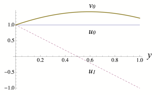
When and , can be large in the whole spacetime by tuning . On the other hand, the conditions , which guarantee the positivity of the lowest scalar-mode mass squared , imply the condition whose r.h.s. should be much less than unity when we request the hierarchy among KK graviton masses. Therefore, we expect that the lowest scalar-mode mass has a large positive value when we set very small and tune , and at the same time we realize the mass hierarchy among KK gravitons. Then, we numerically confirm that we can realize the requested mass hierarchy between the lowest KK graviton mode and the other massive modes. We present the result of the numerical calculation where we set the parameters to be , , , , , and . Figure 1 shows the mode functions , and . The mass eigenvalues are obtained as , and . From the above calculation, we find it possible to construct a higher dimensional model whose low energy effective theory has only two gravitons: one is massless and the other has a tiny mass.
IV linear perturbation in RGT bigravity and DGP two-brane model
In the preceding section, we concluded that we can realize bigravity as the low energy effective theory of DGP two-brane model with an appropriate stabilization mechanism. This effective theory has 7 degrees of freedom in the gravity sector. Whilst, dRGT bigravity, which is constructed for Boulware-Deser not to appear, also has healthy 7 degrees of freedom. If dRGT bigravity is the unique ghost-free bigravity theory, the effective theory of DGP two-brane model should coincide with dRGT bigravity when all massive modes in DGP two-brane model except for the lowest KK graviton are sufficiently heavy and decouple. However, the action of DGP two-brane model (II.1), is not only composed of Ricci scalars with respect to two metrics induced on the respective branes but also contains five-dimensional Ricci scalar in the bulk, whose counterpart seems to be absent in dRGT bigravity. Hence, if we consider higher order in the derivative expansion, the two metrics will have derivative coupling in DGP two-brane model, and the correspondence will not be maintained. Also, in order to obtain bigravity as an effective theory of DGP two-brane model, all massive modes except for the lowest KK mode must be suppressed. Thus, when we consider non-linear perturbation, it would be necessary to consider relatively large magnitude of perturbation. Otherwise, the effect of heavy modes will be larger than the non-linear effect. Hence, it is not clear if we can extend our analysis to non-linear level. For these reasons, instead of pursuing the extension of our analysis to the non-linear perturbation, here we investigate the nonlinear effect just by changing the background energy scale. Below, we consider perturbation around de Sitter brane background with arbitrary energy scale . We will show that two models are identical as long as the linear perturbation is concerned and how the parameters in two models correspond.
IV.1 DGP model
Considering perturbation from the de Sitter brane background caused by the matter on the -brane in DGP model, the metrics induced on the branes become
| (IV.1) |
Following the discussion in Ref. Izumi , from Eqs. (III.3) and (III.6), the metric components induced on the respective branes are obtained as
| (IV.2) | ||||
| (IV.3) | ||||
| (IV.4) |
Since there is no propagating degree of freedom corresponding to , the terms in proportional to should not be present in total. This condition implies an identity
| (IV.5) |
which can be also proven by using the residual gauge transformation and junction condition on the -brane Izumi . Applying the same argument to the junction condition on the -brane, we obtain another identity:
| (IV.6) |
Using these relations the expressions for the induced metrics simplify a lot. Furthermore, for the comparison with the bigravity model, we truncate the expression by keeping only the massless and the lowest mass KK graviton modes. Eliminating the terms that can be erased by four-dimensional gauge transformation, become
| (IV.7) |
We can confirm that the massless mode behaves like the graviton in GR, while the massive mode behaves like the Fierz-Pauli massive graviton.
We can write the metrics induced on the branes as
| (IV.8) | ||||
| (IV.9) | ||||
| (IV.10) |
To find the explicit form of the mode functions, we take the small limit keeping constant, which makes the other KK modes decoupled. In this limit we necessarily have in the normal branch, and hence we approximate and . Under this approximation, using Eqs. (III.12) and (III.13), we obtain , and
| (IV.11) | ||||
| (IV.12) |
The normalization constants and are determined so that the modes are normalized with respect to the inner product (III.2). Keeping the leading order of , the inner product (III.2) is evaluated only by the boundary contributions, and we have
| (IV.13) | ||||
| (IV.14) |
Finally, we obtain the metrics induced on the branes as
| (IV.15) |
IV.2 dRGT bigravity
In this subsection we derive the linearized perturbation equations in dRGT bigravity around de Sitter background. The action of dRGT bigravity is
| (IV.16) |
where and are, respectively, the physical and the hidden metrics. is the 4 dimensional Planck mass for while is that for . is the matter Lagrangian and the matter is assumed to couple only to the physical metric. The interaction between and is given by
| (IV.17) |
with
| (IV.18) | ||||
| (IV.19) |
where we have introduced and .
The equations of motion of dRGT bigravity can be written as
| (IV.20) | ||||
| (IV.21) |
where
| (IV.22) | |||
| (IV.23) |
where .
In the case of de Sitter background, metrics are related to each other as . For simplicity, we define functions and as
| (IV.24) | ||||
| (IV.25) |
where . Denoting the curvature radius of the background physical metric as and the cosmological constant coupled to the physical metric as , the background equations imply
and
We consider linear perturbation , , where is the de Sitter metric with the curvature radius . From Eqs. (IV.20) and (IV.21), we obtain
| (IV.26) | ||||
| (IV.27) |
with , and
| (IV.28) |
where is the covariant differentiation associated with and . Combining Eqs. (IV.26) and (IV.27), we can decompose these two modes into one massless mode and one massive mode . Using the energy conservation law and the Bianchi identity, we obtain
| (IV.29) |
Using Eqs. (IV.26), (IV.27), (IV.28) and (IV.29), the equation of motion for the massive mode becomes
| (IV.30) |
where
| (IV.31) |
Taking the trace of Eq. (IV.30),
| (IV.32) |
The traceless part of Eq. (IV.30) leads
| (IV.33) |
Here we used the identity for an arbitrary scalar ,
| (IV.34) |
The term proportional to in Eq. (IV.33) can be erased by a gauge transformation. Combining Eq. (IV.33) and Eq. (IV.32), we obtain
| (IV.35) |
We also find the equation for the massless mode as
| (IV.36) |
The equations for massive and massless modes in dRGT bigravity (IV.35) and (IV.36) take the same form as the equations in DGP model (IV.9) and (IV.10). We can write two metrics using massless and massive gravitons as
| (IV.37) |
To see the correspondence between the effective bigravity derived from DGP two-brane model and dRGT bigravity, we compare Eq. (IV.15) and Eq. (IV.37). We find that the the metrics on the -brane and the -brane in DGP two-brane model agree with the physical and the hidden metrics in dRGT bigravity if we identify as and . Notice that dRGT bigravity accepts the scale transformation , , . The metric perturbations and are invariant under this transformation, which enables us to arbitrarily rescale the hidden metric .
Let us consider a homogeneous and isotropic perturbation in DGP two-brane model and compare it with the result in ref. GW . We can easily find that the light cone of the metric on -brane changes in the same way as that of the hidden metric in ref. GW , because the induced metric perturbation is identical. In order to see the nonlinear effect by raising the background energy scale as anticipated, we would be able to compare the Friedmann equations. However, it is hard to obtain the Friedmann equation in DGP two-brane model because of the back reaction on the structure of the fifth dimension caused by changing the brane cosmological constant. Furthermore, we find that there is a tachyonic instability in the sector of the stabilization scalar field, which will be shown in the succeeding section, and hence we will not further discuss the non-linear perturbation in this paper.
V Instability
In this section we investigate instabilities in DGP two-brane model with a scalar field for the radion stabilization and those in dRGT bigravity. We will discuss how one can interpret the instabilities in dRGT bigravity from the viewpoint of higher dimensional gravity and the difference in the way how instabilities appear between these two models.
V.1 DGP model
It is known that the self-accelerating branch of DGP two-brane model inevitably has ghost Izumi . Therefore, here we consider the normal branch, which is obtained by a continuous deformation of the model from a rather simple setup that accepts the solution with two Minkowski branes and the bulk satisfying .
Using the eigenfunctions and , we can obtain the solution for the perturbation and induced by the matter on the -brane. As was discussed in Izumi , a KK graviton in the mass range and a spin-0 mode with the mass below become a Higuchi ghost and a scalar ghost, respectively, and lead to quantum instabilities. We begin with Minkowski brane solution and consider to gradually increase the brane tension of the -brane. As we will see below, one can verify that on the background solution obtained in this manner ghost does not arise as long as , thanks to the identity (IV.5). When only small perturbation from this solution is concerned, the mass spectrum will remain to be essentially the same, and therefore all KK graviton masses are above and all spin-0 mode masses are above . Hence, there appears no instability. If we continue to increase the brane tension further, we can obtain de Sitter branes with the four-dimensional Hubble parameter . The mass eigenvalues vary but they must satisfy Eq. (IV.5). The assumption guarantees that the norm of is always positive, and hence is positive. By assumption, the solution remains in the normal branch, in which is satisfied. In this case, when crosses the critical value from above, the first term on the l.h.s. in Eq. (IV.5) diverges to positive infinity. Similarly, when crosses , the first term in the square brackets on the l.h.s. diverges to positive infinity. Whilst, there is no other term that diverges to negative infinity. Therefore the crossing of the critical masses violates the identity (IV.5), and hence it never happens. Hence, the mass spectrum on the background solution constructed in this manner is guaranteed to be free from ghost.
However, Eq. (II.9) implies that, as we increase the brane tension, becomes as large as unless miraculous cancellation by the change of occurs. At least, as long as we consider models in which is pinned down by sufficiently large , this cancellation cannot be expected. Therefore, when is large, becomes larger than and the lowest scalar mass squared crosses just by considering a slightly higher energy regime, . As we increase the brane tension little by little starting with Minkowski branes, becomes negative and the scalar tachyon appears before crosses . This tachyonic instability would mean the boundary whether the spacetime structure with stably separated two branes is sustainable or not. In the presence of the scalar tachyon, two branes will move away from each other further and further, and hence DGP model cannot reproduce the bigravity. To avoid such an instability in the high energy regime, we should invent some other mechanism to stabilize the separation between two branes much more strongly, which is left for future work. Once either of becomes negative, the solution is in the self-accelerating branch. Izumi et al. Izumi proved that we cannot avoid the ghost instability in this branch using the same identity (IV.5), which we used to prove the absence of instability in the normal branch. If we further deform the model, we may have a transition between a scalar mode with and Higuchi ghost, which was discussed in Ref. Izumi .
V.2 dRGT bigravity model
Here we study how ghost appears in dRGT bigravity model. We consider FLRW background and its perturbation in dRGT bigravity. We assume the background geometry as given by
| (V.1) | |||
| (V.2) |
Following the discussion in GW , we select the healthy branch to solve the conservation equation . the equation of motion becomes
| (V.3) |
where , is the matter energy density and
| (V.4) | ||||
| (V.5) |
where . The graviton mass squared is given in Eq. (IV.31) and positive when . According to cos5 , the helicity-0 mode of graviton becomes ghost when is smaller than , which is the so-called Higuchi ghost. After some calculation, we find
| (V.6) |
Therefore, we can judge the appearance of ghost by the sign of . When is negative, the solution is free from the Higuchi ghost.
Suppose that the vacuum energy is tuned so as to possess a vacuum Minkowski solution with and . We consider a branch of the solution that evolves to this Minkowski solution. As we increase the energy density , FLRW solution ceases to exist at the point where . Up to this energy density, remains to be negative as far as is satisfied for . Equation (V.6) tells that is kept to be positive on this branch. Therefore, we can conclude that the cosmological solution constructed in this way has no Higuchi ghost as long as the positivity of the graviton mass squared in the Minkowski limit is guaranteed. On the branch with , the graviton’s mass is less than and the Higuchi ghost appears.
The way how ghost appears in dRGT model is clearly different from the case in DGP model. In the dRGT bigravity, before the Higuchi ghost appears, there is no instability, while in DGP model the onset of the instability is tachyonic. We can understand this disagreement as caused by the truncation of the scalar mode. On one hand, in DGP two-brane model the scalar modes could be effectively neglected when all of them are sufficiently heavy. However, once some of them become light, we cannot neglect them any more. Hence, we found a tachyonic instability. On the other hand, in dRGT bigravity scalar modes do not exist from the beginning. Therefore, the appearance of the tachyonic scalar mode observed in DGP two-brane model does not show up in the corresponding dRGT bigravity, which keeps dRGT bigravity “healthy” even in the energy regime higher than .
VI Summary
In this paper, we have investigated whether or not dRGT bigravity can be embedded in higher dimensional gravity. Here, we have considered DGP two-brane model with sufficiently large brane induced gravity terms and Goldberger-Wise radion stabilization. We have chosen the model parameters so as to accept background solutions in which the brane separation is sufficiently small compared with the length scale determined by the ratio between five-dimensional and four-dimensional Newton’s constants. We have proved that DGP two-brane model in such regime can reproduce bigravity as its low energy effective theory with the help of the stabilization mechanism. Namely, almost massless degrees of freedom in the gravity sector are composed of one massless graviton and one massive graviton with a small mass.
DGP model is known to have the normal branch and the self-acceleration branch. We clearly identify the condition to distinguish these two branches in the setup with a scalar field introduced for the purpose of radion stabilization. We succeeded in proving that the model does not have ghost as long as the normal branch solution is chosen. Putting aside the issue of Higuchi ghost, since DGP two-brane model does not have ghost in the scalar-type perturbation irrespective of the choice of branch, the ghost corresponding to BD ghost in bigravity is guaranteed to be absent. Therefore, the low energy effective theory of DGP two-brane model is expected to be identical to dRGT bigravity, which is the unique bigravity theory that is free from BD ghost. As is expected, we also succeeded in proving this identity, at least, at the linear level.
We have also studied how ghost appears in DGP two-brane model and dRGT bigravity when we continuously modify the model parameters. In both models we can consider backgrounds that are free from ghost at low energies. In DGP two-brane model with stabilization, however, it is difficult to avoid ghost when we slightly increase the background energy scale. This is because the stabilization of the brane separation is hard to maintain as long as we keep the conditions for the normal branch. As a result, a tachyonic four-dimensional scalar mode arises. By contrast, in dRGT bigravity such a four-dimensional scalar degree of freedom corresponding to the brane separation does not exist from the beginning, and hence the model remains free from the instability. Therefore, it turned out that the correspondence between DGP two-brane model with scalar-field stabilization mechanism and dRGT bigravity holds only in the very limited low energy regime.
Unfortunately, because of this instability that occurs at a relatively low energy, it is difficult to fully justify investigating the properties of dRGT bigravity by using the counterpart in the braneworld setup. Nevertheless, it is suggestive to point out that the Vainshtein mechanism in the low energy regime of dRGT bigravity explored in Ref. GW tells that the physical and hidden metrics are similarly excited near gravity sources. It might be natural to expect that the same feature will arise for the metrics induced on both branes when the brane separation is very small. The effective gravitational coupling that appears in the effective Friedmann equation and the local Newton’s law within the Vainshtein radius in the low energy regime of dRGT bigravity is given by the sum of the four-dimensional Planck mass squared for the physical and the hidden metrics. This feature can also be understood as the dilution of gravitational force line, which is very familiar in the braneworld context. In our future publication we will study whether or not there is more efficient stabilization mechanism that maintains the correspondence even in the higher energy regime.
Acknowledgements This work was supported in part by the Grant-in-Aid for Scientific Research (Nos. 21244033, 21111006, 24103006 and 24103001). We also would like to mention that the discussion during the molecule-type YITP workshop: YITP-T-13-08 was useful to complete this work.
References
- (1) S. F. Hassan and R. A. Rosen, JHEP 1202, 126 (2012).
- (2) . G. Boulware and S. Deser, Phys. Rev. D 6, 3368 (1972).
- (3) C. de Rham and G. Gabadadze, Phys. Rev. D 82, 044020 (2010).
- (4) C. de Rham, G. Gabadadze and A. J. Tolley, Phys. Rev. Lett. 106, 231101 (2011).
- (5) S. F. Hassan and R. A. Rosen, Phys. Rev. Lett. 108, 041101 (2012).
- (6) M. S. Volkov, JHEP 1201, 035 (2012).
- (7) D. Comelli, M. Crisostomi, F. Nesti and L. Pilo, JHEP 1203, 067 (2012) [Erratum-ibid. 1206, 020 (2012)].
- (8) D. Comelli, M. Crisostomi and L. Pilo, JHEP 1206, 085 (2012).
- (9) A. De Felice, A. E. Gumrukcuoglu and S. Mukohyama, Phys. Rev. Lett. 109, 171101 (2012).
- (10) M. Fasiello and A. J. Tolley, JCAP 1312, 002 (2013).
- (11) M. S. Volkov, Phys. Rev. D 85, 124043 (2012).
- (12) E. Babichev and A. Fabbri, Class. Quant. Grav. 30, 152001 (2013).
- (13) A. De Felice, T. Nakamura and T. Tanaka, arXiv:1304.3920 [gr-qc].
- (14) L. Randall and R. Sundrum, Phys. Rev. Lett. 83, 3370 (1999).
- (15) L. Randall and R. Sundrum, Phys. Rev. Lett. 83, 4690 (1999).
- (16) G. R. Dvali, G. Gabadadze and M. Porrati, Phys. Lett. B 485, 208 (2000).
- (17) A. Padilla, Class. Quant. Grav. 21, 2899 (2004).
- (18) W. D. Goldberger and M. B. Wise, Phys. Rev. Lett. 83, 4922 (1999).
- (19) S. Kanno and J. Soda, Phys. Rev. D 66, 043526 (2002).
- (20) K. Izumi, K. Koyama and T. Tanaka, JHEP 0704, 053 (2007).
- (21) O. DeWolfe, D. Z. Freedman, S. S. Gubser and A. Karch, Phys. Rev. D 62, 046008 (2000).