Diversity of scales makes an advantage: the case of the Minority Game
Abstract
We use the Minority Game as a testing frame for the problem of the emergence of diversity in socio-economic systems. For the MG with heterogeneous impacts, we show that the direct generalization of the usual agents’ profit does not fit some real-world situations. As a typical example we use the traffic formulation of the MG. Taking into account vehicles of various lengths it can easily happen that one of the roads is crowded by a few long trucks and the other contains more drivers but still is less covered by vehicles. Most drivers are in the shorter queue, so the majority win. To describe such situations, we generalized the formula for agents’ profit by explicitly introducing utility function depending on an agent’s impact. Then, the overall profit of the system may become positive depending on the actual choice of the utility function. We investigated several choices of the utility function and showed that this variant of the MG may turn into a positive sum game.
keywords:
Minority Game , econophysics , stochastic processesPACS:
89.65.-s , 05.40.-a , 05.65.+b1 Introduction
The Minority Game (MG), introduced slightly more than a decade ago [1, 2, 3, 4, 5], gained the reputation of an “Ising model” in the field of Econophysics [6, 7]. It is surely an exaggeration, as the complexity of the Ising model is many orders of magnitude higher, but nevertheless, the MG is a widely accepted framework for testing a variety of ideas in modelling socio-economic phenomena. There are several excellent reviews [8, 9, 10, 11] of the vast literature on the subject, which we have no intention to review again here. The aim of our work is to contribute to understanding the possible advantages of diversity, which may be one of the sources of the heterogeneity of agents.
The topic of our work falls within the generalisations of the canonical MG to the case of several different groups of agents. Perhaps the most deeply studied is the variant with two types of agents, called producers and speculators [12, 13, 14]. The market ecology which emerges, shows fairly clearly that the two groups need each other to gain better efficiency. In different perspective, the agents may be divided into groups of leaders and imitators [15, 16, 17, 18]. Here also, the performance of the system as a whole might be increased, if the imitators are present in proper fraction. If the agents are allowed to participate in the game or not, depending on their score [19, 20, 21, 22], the bursts of activity reminiscent of the effect of volatility clustering are observed. Similar case considers agents who play the game at certain fixed frequency. Their frequencies may be broadly distributed, which induces new features into the game [23, 24, 25]. The case of investors with different weights was investigated for a very general setup [26]. In our work, we choose a more specific situation and show that it leads to new non-trivial consequences.
From the following consideration it can be seen why can be the diversity helpful in the framework of the MG. In the traffic formulation of the MG, the drivers choose between two alternative roads and those who take the less crowded one, are the winners. If all the vehicles have the same length, only minority of agents can be counted winners, namely those who drive on the road with minority of drivers. However, imagine that besides trucks, there are also small city cars. It can easily happen that one of the roads is crowded by a few long trucks and the other contains more drivers but still is less covered by vehicles. Most drivers are in the shorter queue, so the majority win. This is the essence of our paper which is just mathematical elaboration of this consideration.
However, the previous simple setting does not take into account the utility of the vehicles. In this view, the drivers could choose infinitesimally short vehicles as optimal which clearly contradicts the real traffic situation. Indeed, the longer the car is, the more passengers or load it can carry, obviously for the price of higher fuel consumption. To model these considerations, we incorporated the utility of the vehicles expressed as a function of their length. This way we included feature which favour vehicles of finite length. Nevertheless, the ultimate motivation for the introduction of the utility function is the optimization problem the agents face. We consider the impacts as parameters the agents can choose to maximize their expected utility.
2 Heterogeneous groups in the MG
Generally, the MG is a model of the bounded sources allocation which is driven by agents with bounded rationality. In the simplest setting, they do not have but two options. In each round, they aim to choose the right action, i.e. the action chosen by the minority of agents. Then, only the minority of agents can win for principal reasons. To adapt to their environment, each agent has two strategies. They predict the next optimal choice considering only a few previous results. Still, there is not any space for an adaptation of agents as both their strategies are fixed. Therefore, each agent counts the score of each strategy and then follow the currently better strategy.
In the urban traffic, drivers have cars of various lengths. Following this paradigm, we assign each agent an individual impact on the game. It can be directly interpreted as the length of the vehicle the agent is driving, however, some more ambitious interpretations are left to the conclusion. Next, we divide the agents into several groups according the assigned impacts. Formally, we have groups of agents. The group contains agents and each of them has impact . The total number of agents is and the relative size of group will be denoted . For further convenience, we introduce the following symbol for the weighted average of an arbitrary function over all groups
| (1) |
Throughout this paper, we shall refer to an actual values of the groups’ ratios and impacts as the configuration of the game. To restore the canonical MG, it suffices to set , and equal to .
As usual in the MG, all agents are subject to the same external information and all of them are able to distinguish different information (or memory) patterns . These patterns arrive randomly with uniform probability. We stress that throughout this paper we shall work within batch MG with uniformly distributed random memories, i.e. all P patterns occur with equal frequency, the occurrence of patterns is uncorrelated in time and strategies’ scores are updated only after all patterns are used. Within such setting we can relatively easily obtain analytical results, with no need to resort to computer simulations. In so doing, we rely on the results of Refs. [37] and [38], which show that MG with random uniformly chosen memories is very close, although not identical, to the canonical MG. All important qualitative aspects are the same and the small quantitative difference diminishes when we approach the critical point.
In sequel, we shall denote the average of a function taken over all the information patterns as . Next, the action prescribed by strategy of -th agent from group , provided the information pattern is , is denoted by . Then, the currently executed action of an agent reads
| (2) |
where the random variable is an agent’s current choice of strategy. It will be specified in detail later on. The following combinations
| (3) |
allow us to write the aggregated action of agents from group as
| (4) |
Next, for the overall impact of all individual actions of all agents we have
| (5) |
We follow the batch variant of the MG where the difference of strategies’ scores evolves as
| (6) |
Note that in this definition the update of the strategies’ scores of an agent contains just the variable indicating the chosen side. The alternative updating of the score would be proportional to the impact of the agent in question. We shall discuss the differences between these two choices later.
Now, the current strategy choice of an agent is governed by the stochastic rule
| (7) |
where the parameter is usually named as the “learning rate”. Indeed, the higher the value of is, the more an agent trust his current knowledge represented by the value of . Henceforth, we denote the mean value of any random variable with respect to the probability distribution (7) by angular brackets, . Especially, for the mean value of itself, we have
| (8) |
In what follows, we shall refer this value as magnetization in analogy to purely physical systems.
In the next section, these magnetizations are necessary to evaluate the performances of the agents in the MG. Optimally, we would calculate all as functions of time and made our conclusions. To ease this program a bit, we utilize here the pioneering way the MG was firstly solved using the replica method [30, 31]. Thus, we search for the value of only at the stationary point of the game’s dynamics. Such stationary value is defined in this manner
| (9) |
The same convention will be used also for other variables to denote their stationary value.
To find the stationary state, we observe that, for , the evolution of the strategies’ scores (6) implies the following dynamics of magnetizations (8)
| (10) |
with the Lyapunov function
| (11) |
which plays the role of the Hamiltonian in subsequent calculations. Next, by calculating the arguments of the minimum of we obtain the stationary values of .
If we make the score updates proportional to the actual impact of an agent, which is the alternative already discussed nearby Eq. (6), the equation (10) would require a modification. However, a short calculation reveals that the modification consists only in missing in the denominator on the right-hand side of Eq. (10). Most importantly, both definitions result in the same Lyapunov function and further course of the calculations is therefore identical. Thus, it does not matter whether the prescription for the dynamics of strategies’ scores (6) is proportional to an actual impact or not. However, what does matter, is the definition of the outcome of the game for an agent, as defined later in Eq. (14). The choice (6) we did earlier was taken to make this definition conform with the definition (14) (to be seen later).
In fact, the previous approach with Hamiltonian playing the role of Lyapunov function is not the most general. To determine the behaviour of the MG for arbitrary , there exists another path of calculations mastering stochastic calculus [32]. However, it was shown that finite value of influences the results only in the non-ergodic phase while in the ergodic phase the results are independent of . Here we investigate only the ergodic phase, thus the limit is acceptable and the use of Lyapunov function is justified.
In the course of computations, we shall work in the thermodynamic limit of infinite number of agents, , keeping all group ratios fixed, and at the same time limiting the number of information patterns to infinity, , holding the fraction
| (12) |
fixed. This value is the principal parameter of both canonical and generalized MG.
3 The profit of agents
In this section, we have to detour from the conventional notation used in the context of the MG. To incorporate the utility function of agents, it is better to write about their profits instead of their losses. To establish the connection to the canonical MG, a clear relation to volatility
| (13) |
which is the usual characteristic of agents’ performance, will be derived.
First of all, we define the current outcome of an individual agent of group as
| (14) |
It indicates whether an agent was successful in the current round of the batch MG. His ability to obey the “join-minority imperative”, i.e. to choose for a typical information pattern , guarantees him positive outcome and the same holds vice versa. We note that the fact that an agent’s impact is not included in formula (14) is the crucial point of our modification of the MG.
Next, for the average outcome within the group we have
| (15) |
Coming to the stationary state, we can write (the stationary value of) the overall average outcome as
| (16) |
To relate an average outcome within a group to an average profit of that group, we have to take into account the utility function . We follow the standard way it is defined in classical economics. Its purpose is to quantify agents’ preferences over the whole spectra of possible impacts [36]. In other words, the more an agent prefers impact , the higher value is assigned to that impact by . Such utility function can be interpreted, for instance, as the profit of an owner of the vehicle of length . For the sake of simplicity, we assume that the utility function is common for all agents of all groups and non-negative. Now, we define the average profit of group provided the utility function is in this manner
| (17) |
Then, the overall average profit over all groups reads
| (18) |
We note that introduction of is by no means equivalent to readjusting of the impacts.
If we consider all impacts to have the same utility, i.e. , we obtain an extremal case of profit . On the other hand, prescribing an utility of impact directly proportional to its size, i.e. , we observe , so the minus volatility (13) is another extremal case of the profit defined by formula (18). Realistic situations will lie somewhere in the middle. For example, we can choose for or . However, in the following we shall mainly compare the extremal cases and , to better see the difference. We shall see that this shift of focus has important implications on the conclusions we shall draw from the results of the computations.
At the moment, we define the mutual predictability between groups
| (19) |
which is a direct generalisation of the usual definition of the predictability in the canonical MG [9]. It corresponds to the ability of group to adapt to the aggregated attendances , and vice versa. The less the value of is, the more the groups are adopted to each other as their aggregated attendances and are more anti-correlated. Then, for the mean predictability of group it holds
| (20) |
Its knowledge is the key ingredient in the calculation of . Indeed, if we apply the approximation
| (21) |
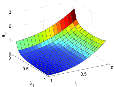
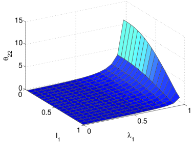
which is justified in the ergodic phase, see again Ref. [9], introduce the set of order parameters for
| (22) |
and compare definitions of and , see (15) and (20), respectively, we obtain
| (23) |
At this moment, we can realise the importance of . It is not only a characteristic of groups’ ability to predict the overall impact , but it is also a link connecting the knowledge of the outcome of group to the knowledge of the minima of Hamiltonian . Recalling the definition of , see (19), together with equation (11), we can derive that
| (24) |
Thus, as soon as we know as function of the impacts , , we deduce also all mean predictabilities for all groups using the mutual predictabilities .
4 Replica solution
Whatever utility function we choose for the impact of the agents, the key elements for the calculation are the average groups’ outcomes which are functions of the stationary magnetizations , see (23). To obtain these magnetizations, it suffices to minimise the Hamiltonian as it is also Lyapunov function for their dynamics, remember equation (10). The technical obstacle to actual computation consists in the quenched disorder contained in the Hamiltonian (11) due to the random strategies . The standard procedure to tackle this complication is the replica method [28, 29].
To briefly depict this method, consider a system with Hamiltonian dependent on state variable and also on random, but quenched disorder distributed with probability . In that setting, even the partition function is a random variable and so is the free energy . Then, the physically relevant quantity is the mean free energy . To ease its computation, the replicated partition function is introduced as the central notion of this method. It is calculated by replicating the system -times with the same disorder , and finally, by taking an average over this disorder
| (25) |
As the second equality indicates, is also a characteristic function for the random variable . Thus, for the mean free energy it holds
| (26) |
However, this limiting process is only formal as we are unable to calculate for general , except for positive integers. The existence and uniqueness of an analytical continuation of is an open question of the contemporary mathematical physics.
Full solution of the canonical MG using replica method is available [30, 31], as well as solution of various modifications of the MG [13, 14, 23, 25, 33, 34, 35]. We apply this method straightforwardly to our case. For the replicated partition function we obtain formula
| (27) |
where the sum goes over all possible realizations of the quenched disorder. Using Hubbard-Stratonovich transformation, we introduce auxiliary variables indexed by replica index . Thus, we obtain the previous formula in the following form
| (28) |
To compute it, it is necessary to introduce the replica-symmetric ansatz and then apply the saddle-point method. Next, we calculate the mean free energy using equation (26). Finally, to achieve the formula for the minima of Hamiltonian , it suffices to carry out the following limit
| (29) |
Without resorting more details of the computation, we note that at the core there is an equation for an auxiliary quantity parameterized by defined in (12)
| (30) |
Once is found, we can calculate the order parameters
| (31) |
the minimum value of the Hamiltonian
| (32) |
and hence the mutual predictability using relation (24) reads
| (33) |
Considering equation (23), we conclude
| (34) |
The expression (34) is the main result we shall build on further in the following sections. Before going to that, we complete the calculations by the formula for the volatility (13) which is
| (35) |
In the following two sections, we shall analyse these results first at the critical point and then deep in the ergodic regime.
5 Critical behaviour
For the minimization of the analysis of critical behaviour is crucial. The calculation of (27) is valid only in the ergodic phase of the MG as it was already examined in Ref. [9]. Therein, the formula for susceptibility is obtained which in our setting directly generalizes to
| (36) |
And it is the very fact of diverging susceptibility what characterises the critical point. Thus, it was deduced that the ergodic phase of the MG corresponds to values with the critical value obtained from
| (37) |
with given by an equation emerging from the previous equation together with (30)
| (38) |
Considering only one group of players, critical coefficient of the canonical MG reappears. Generally, the critical value is equal or below this “canonical” value for any game configuration due to the concavity of in (37).
In the canonical MG, the predictability vanishes at the critical point . This observation does not hold for the mutual predictabilities directly, however, it holds for the mean predictability of an arbitrary group . To verify it, we substitute condition (37) for into the definition of , see (20), using equation (33). The achieved equation for at the critical point is directly proportional to the left side of (38) and on that account does vanish here.
Another significant characterization of the critical point in the canonical MG was related to the notion of frozen agents firstly mentioned in Ref. [39]. An agent of group is called frozen if one of his strategies is significantly better than the other. Thus, in the stationary point it holds . In the canonical MG the fraction of frozen agents is maximized at the critical point and it decreases with increasing . For the fraction of frozen agents within group in the MG with heterogeneous impacts we obtain
| (39) |
following Ref. [40]. Then, the overall fraction of frozen agents is
| (40) |
From equation (30) we can see that grows with increasing . Thus, even in the MG with heterogeneous impacts the overall ratio of frozen agents is maximized at and decreases with increasing . Furhtermore, this observation holds regardless of the actual game configuration .
Also, the loss in the canonical MG, which is represented by volatility , was minimized at the critical point. We will show that this fact is violated in the generalized MG. Substituting the condition (37) for into the formula for a group outcome , remember (15), we obtain a simplified formula at the critical point
| (41) |
We can show that holds for all groups and all the possible game configurations as long as we are at the critical point. It implies that even the average profit is negative here for an arbitrary utility function (which is non-negative by definition). Nevertheless, in the next section, we will see that there exist game configurations where holds for some specific utility functions away from the critical point. The existence of positive average profits away from critical point implies that the critical point is no more optimal for the generalized variant of the MG. However, this observation depends on the considered utility function.
6 Two groups
Next, we examine the easiest generalisation of the canonical MG. We consider a game consisting of two groups of agents, , and depict their co-habitation. Firstly, we fix a scale of impacts
| (42) |
This particular choice establishes a relation to the canonical MG as corresponds to volatility in the game of randomly guessing agents. Thus, having this normalisation, we work on the scale of the canonical MG. We also prefer this normalisation because the calculations for the game with infinitely many groups are valid only provided [26].
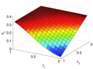
In all the subsequent figures it suffices to consider impact since the rest of function values, i.e. those of argument , are determined through (42) by reversing the groups. As for the variable , we restrict ourselves to . It is possible to prove that is discontinuous along the line considering the normalisation (42). In Fig. 2, it is clearly visible that the critical value is, indeed, lower or equal to the critical value observed in the canonical MG. We picked for all subsequent calculations in order to remain safely in the ergodic phase as it was discussed in the previous section.
The principal novelty in our result is that for some game configurations the overall average outcome can even be positive as depicted in Fig. 2. In other words, the majority of agents wins in these cases. From Fig. 4 and Fig. 4 showing separate outcomes of each group and , respectively, we can deduce what is behind this phenomena. To gain on average, one group has to sponge off the other. In the case of two groups, the group with smaller impact is always winning. Its positive outcome is not very high, in fact, but when weighted by the groups’ ratios, it can overweight negative outcome of the other group.
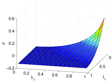
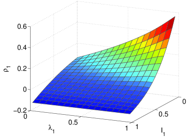
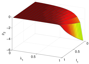
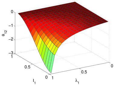
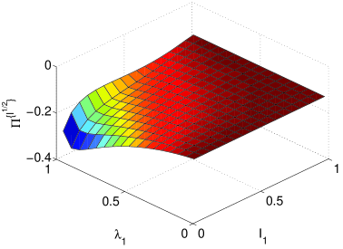
In the next three figures, we plot the predictabilities , and mutual predictability , see Fig. 6, Fig. 6 and Fig. 8, respectively. Note that the positiveness of the diagonal elements of is enforced by their definition, see (19). Next, we observe that is negative for all configurations of the game. In other words, the aggregated actions and are anticorrelated for the MG consisting of two groups.
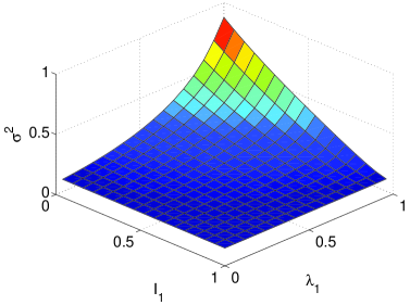
In Fig. 8, we show the volatility defined by (13). The closer is to , the closer is the result of the game to the behaviour of randomly guessing agents. We observe that this holds in the vicinity of and . In other words, the co-adaptation of agents is poor for these game parameters. However, it is the same area where falls almost to , confer Fig. 2. It resembles a similar feature of the canonical MG, where grows with receding from . Here, the situation is analogous. Even though was fixed in this set of calculations, is decreasing in the region of our interest and thus the distance is growing.
The next three figures depict the fraction of frozen agents. We plot their overall fraction , fraction of frozen agents within the first group and fraction of frozen agents within the second group , see Fig. 10, Fig. 10 and Fig. 12, respectively. For higher ratio of frozen agents we observe also the higher overall outcome, compare with . This was valid also in the canonical MG, where frozen agents were more effective on average.
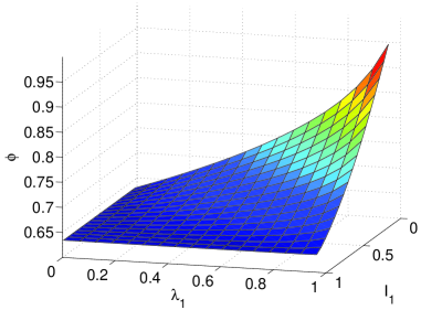
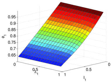
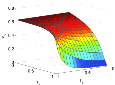
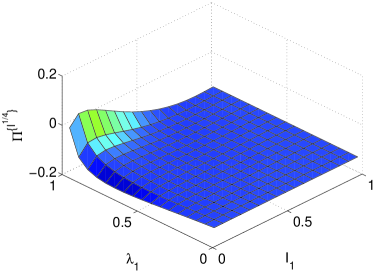
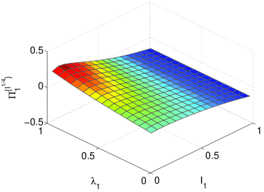
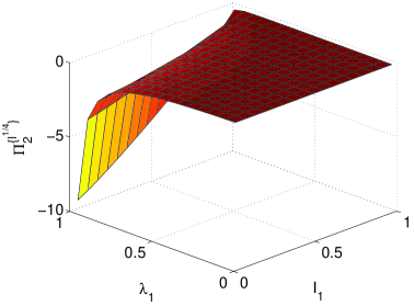
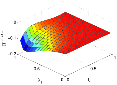
In the last set of figures, we depict the way the overall average profit is influenced by the particular choice of the utility function . The overall average profits and are depicted in Fig. 12 and Fig. 14, respectively. For the utility function we append Fig. 14 and Fig. 16 depicting a separate average profits of both groups and , respectively. Next, we add another overall average profit using a different shape of the utility function, see Fig. 16. For all these utility functions new local maxima of appear.
Although we did not solve explicitly the problem of maximizing the agents’ utility, we consider the calculated dependence of the average profit on impacts as a guide for a hypothetical choice of optimal impact. The location of the optimum depends crucially on the form of the utility function. Therefore, the introduction of the utility function is one of the cornerstones of our approach.
7 Conclusion
We investigated in detail the modification of the Minority Game in which the agents act on different scales. These heterogeneous scales are implemented as agents’ impacts and can be interpreted in different ways. Within the traffic metaphor of the MG, the impacts corresponds to the lengths of the vehicles the agents are driving. Alternatively, we can view it as a simplified method how to account for different frequencies at which the agents are playing. Then, an agent’s impact is directly proportional to the inverse of the time scale at which the agent is participating.
The agents are divided into several groups according to their impacts. The MG model with heterogeneous impacts is solved by standard procedure using the replica trick. The average outcome of each group was then obtained, as well as the mutual predictabilities of the groups. To interpret properly the ensemble of outcomes for each group, we introduce an utility function of the impact of agents. Within the traffic metaphor, utility says how much profit can be expected having vehicle of the given length. The average profit of individual groups is calculated from their average outcomes, with utility considered. We discuss the overall average profit of the system for the simplest case of two groups. The agents with lower impact are always in advantage, and the overall profit of the system can even be positive, which means that the MG viewed from this perspective may be a positive-sum game. This is in contrast with the usual way of measuring the losses through the volatility which enforces that the MG is a negative-sum game.
Although we kept the traffic metaphor of the MG within this paper, we believe that the results can be interpreted also in the language of stock markets. We argue that if we think of the impact of an agent as the size of the capital an investor is playing with, the relative outcome is more suitable description of an agent’s profit. The real investors do compete for highest relative rather than absolute profit. We see that in absolute numbers the MG with heterogeneous impacts remains, of course, a negative-sum game, but subjectively felt relative profit of agents averaged over the whole system may be positive. This observation could give a cause for the heterogeneity of investors’ sizes, which is one of the most fundamental features of the stock market [27]. Interpreting the utility function as an investor’s subjective evaluation of the capital unit , the notion of is a tool suitable for finer analysis of this phenomena.
To sum up, by introduction diversity in the impact of agents, the average profit in the MG, measured by an non-negative utility function, may turn the MG into a positive-sum game, so that the diversity implies advantage for all. We can conjecture that this is the driving mechanism which favours emergence of groups acting with different impacts. An important question which still remains to be solved is, what would happen if each of the agents is free in her choice of the impact. Both group sizes and group impacts would be free to be adjusted to an optimum. The investigation of the properties of these Nash equilibria is left to a future publication.
Acknowledgements
We want to thank Y.-C.Zhang for giving us the original motivation for this research. We acknowledge constructive remarks of Ing. Miroslav Kárný, DrSc., who helped us to improve the manuscript. This work was carried our within the project AV0Z10100520 of the Academy of Sciences of the Czech republic and was supported by the MŠMT of the Czech Republic, grant no. OC09078 and by the GA ČR grant no. 102/08/0567.
References
- [1] W. B. Arthur, Amer. Econ. Review (Papers and Proceedings) 84 (1994) 406.
- [2] D. Challet and Y.-C. Zhang, Physica A 246 (1997) 407.
- [3] D. Challet and Y.-C. Zhang, Physica A 256 (1998) 514.
- [4] N. F. Johnson, S. Jarvis, R. Jonson, P. Cheung, Y. R. Kwong, and P. M. Hui, Physica A 258 (1998) 230.
- [5] R. Savit, R. Manuca, and R. Riolo, Phys. Rev. Lett. 82 (1999) 2203.
- [6] R. N. Mantegna and H. E. Stanley, Introduction to Econophysics: Correlations and Complexity in Finance (Cambridge University Press, Cambridge, 1999).
- [7] J.-P. Bouchaud and M. Potters, Theory of Financial Risk and Derivative Pricing (Cambridge University Press, Cambridge, 2003).
- [8] N. F. Johnson, P. Jefferies, and P. M. Hui, Financial Market Complexity, (Oxford University Press, Oxford, 2003).
- [9] D. Challet, M. Marsili, and Y.-C. Zhang, Minority Games, (Oxford University Press, Oxford, 2005).
- [10] A. C. C. Coolen, The Mathematical Theory of Minority Games, (Oxford University Press, Oxford, 2005).
- [11] A. De Martino and M. Marsili, J. Phys. A: Math. Gen. 39 (2006) R465.
- [12] F. Slanina and Y.-C. Zhang, Physica A 272 (1999) 257.
- [13] D. Challet, M. Marsili, and Y.-C. Zhang, Physica A 276 (2000) 284.
- [14] D. Challet, M. Marsili, and Y.-C. Zhang, Physica A 294 (2001) 514.
- [15] F. Slanina, Physica A 286 (2000) 367.
- [16] F. Slanina, Physica A 299 (2001) 334.
- [17] M. Anghel, Z. Toroczkai, K. E. Bassler, and G. Korniss, Phys. Rev. Lett. 92 (2004) 058701.
- [18] H. Lavička and F. Slanina, Eur. Phys. J. B 56 (2007) 53.
- [19] Y.-C. Zhang, Europhysics News 29 (1998) 51.
- [20] P. Jefferies, M. Hart, P. M. Hui, and N. F. Johnson, Eur. Phys. J. B 20 (2001) 493.
- [21] I. Giardina, J.P. Bouchaud, and M. Mézard, Physica A 299 (2001) 28.
- [22] D. Challet and M. Marsili, Phys. Rev. E 68 (2003) 036132.
- [23] M. Marsili and M. Piai, Physica A 310 (2002) 234.
- [24] A. De Martino, Eur. Phys. J. B 35 (2003) 143.
- [25] G. Mosetti, D. Challet, and Y.-C. Zhang, Physica A 365 (2006) 529.
- [26] D. Challet, A. Chessa, M. Marsili, and Y.-C. Zhang, Quantitative Finance 1 (2001) 168.
- [27] X. Gabaix, P. Gopikrishnan, V. Plerou, and H. E. Stanley, Nature 423 (2003) 267.
- [28] M. Mézard, G. Parisi, and M. A. Virasoro, Spin Glass Theory and Beyond (World Scientific, Singapore 1987).
- [29] V. Dotsenko, An introduction to the theory of spin glasses and neural networks (World Scientific, Singapore, 1995).
- [30] D. Challet, M. Marsili, and R. Zecchina, Phys. Rev. Lett. 84 (2000) 1824.
- [31] M. Marsili, D. Challet, and R. Zecchina, Physica A 280 (2000) 522.
- [32] M. Marsili and D. Challet, Phys. Rev. E 64 (2001) 056138.
- [33] A. De Martino and M. Marsili, J. Phys. A: Math. Gen. 34 (2001) 2525.
- [34] A. De Martino, I. Giardina, and G. Mosetti, J. Phys. A: Math. Gen. 36 (2003) 8935.
- [35] D. Challet, A. De Martino, M. Marsili, J. Stat. Mech. (2006) P03004.
- [36] S. Barbera, P.J.Hammond, Ch. Seidl, Handbook of Utility Theory, Volume 1, Principles, (Kluwer Academic Publishers, Boston, 1998).
- [37] , A. Cavagna, Phys. Rev. E 59 (1999) R3783
- [38] D. Challet and M. Marsili, Phys. Rev. E 62 (2000) 1862
- [39] D. Challet and M. Marsili, Phys. Rev. E 60 (1999) R6271
- [40] N. Brunel and R. Zecchina, Phys. Rev. E 49 (1994) R1823