Classical Casimir-Polder force between polarizable microparticles and thin films including graphene

Abstract

We derive analytic expressions for the classical Casimir-Polder free energy and force for a polarizable (magnetizable) atom (microparticle) interacting with thin films, made of different materials, or graphene. It is shown that for an isolated dielectric film the free energy and force decrease quicker with separation, as compared to the case of atom interacting with a thick plate (semispace). For metallic films some peculiar features depending on the model of a metal used are analyzed. For an atom interacting with graphene we demonstrate that at room temperature the classical regime is achieved at about $1.5\,\mu$m separation. In this regime the contributions to the free energy and force due to atomic magnetic polarizability are suppressed, as compared to main terms caused by the atomic electric polarizability. According to our results, at separations above $5\,\mu$m the Casimir-Polder interaction of atoms with graphene is of the same strength as with an ideal-metal plane. The classical interaction of atoms with thin films deposited on substrates is also considered.

I Introduction

The Casimir-Polder interaction between polarizable atoms or other microparticles and a cavity wall has long been investigated 1 ; 2 ; 3 . A renewed interest to this subject was generated by the experiments on quantum reflection 4 ; 5 ; 6 and Bose-Einstein condensation 7 ; 8 ; 9 . As a result, the dependence of the Casimir-Polder force on atomic characteristics and material properties of the wall was investigated in detail 10 ; 11 ; 12 ; 13 ; 14 ; 15 on the basis of the Lifshitz theory 2 . Measurements of the thermal Casimir-Polder force between a condensate of ⁸⁷Rb atoms and a SiO₂ plate 15a were used to obtain constraints on the Yukawa-type corrections to Newtonian gravitational law in the micrometer interaction range 15b . Much attention was paid also to atom-wall interaction for the case of electric and magnetic polarizable (i.e., magnetizable) atom near a magnetodielectric wall 16 ; 17 ; 18 . In parallel with atom-wall interaction, there was an increasing interest to the interaction of nanoparticles with material surfaces 19 ; 20 ; 21 ; 22 . Specifically, it was shown 20 that interaction between a nanosphere of radius $1\,\mbox{nm}\leq R\leq 20\,$nm and a metallic plane spaced at a separation $a$ is well described by the Lifshitz formula for atom-wall interaction under a condition $a\geq 100R$. Keeping in mind that nonmagnetic metallic nanoparticles can have relatively large magnetic polarizability due to eddy currents 23 , the respective Casimir-Polder force can be much larger than in the case of atoms.

With discovery of graphene and other carbon nanostructures (see reviews in Refs. 24 ; 25 ) a lot of attention has been paid to the interaction of these nanostructures with atoms, molecules and other microparticles 26 ; 27 ; 28 ; 29 ; 30 ; 31 ; 32 ; 33 ; 34 ; 35 ; 35a . This was motivated by both fundamental interest and prospective applications, e.g., to the problem of hydrogen storage 31 ; 34 . After developing the Dirac model of graphene (see Ref. 24 for a review), it was applied to calculate the van der Waals and Casimir interactions between two graphene sheets and between a graphene and a plate made of ordinary materials 36 ; 37 ; 38 ; 39 ; 40 ; 41 . The obtained reflection coefficients of electromagnetic oscillations on graphene were used to calculate the Casimir-Polder interaction of graphene with different atoms 42 ; 43 ; 44 ; 45 . In so doing the two theoretical approaches have been elaborated. In the framework of one approach the reflection coefficients are expressed in terms of the components of the polarization tensor in (2+1)-dimensional space-time 36 ; 38 ; 40 ; 41 ; 42 ; 43 ; 44 . In the framework of another approach they are effectively expressed in terms of the density-density correlation functions 37 ; 39 ; 45 .

In this paper we find the classical limit of the thermal Casimir-Polder force acting between a polarizable (magnetizable) atom or a microparticle and a thin film made of various materials (isolated or deposited on a substrate). We also replace a thin material film of some thickness with a two-dimensional graphene sheet described using the Drude model and compare the results obtained. The consideration of the classical limit (i.e., the case of sufficiently large separations or high temperatures when the main contribution to the force does not depend on the Planck constant 46 ) allows to obtain all the results in a straightforward analytic form. This simplifies the comparison and helps to reveal the physical role of film thickness. We consider both magnetodielectric and metallic films and find that the dominant contribution to the free energy and force for graphene is in agreement with the case of nonmagnetic metallic films. It is shown that the magnetic properties of a microparticle have no impact on the Casimir-Polder interaction with graphene.

The paper is organized as follows. In Sec. II we introduce the general formalism and consider the classical Casimir-Polder interaction of an electrically and magnetically polarizable microparticle with an isolated magnetodielectric film. In Sec. III the same problem is solved for the case of metallic film characterized by the dielectric permittivity $\varepsilon(\omega)$ and magnetic permeability $\mu(\omega)$. Section IV is devoted to the classical Casimir-Polder interaction of a microparticle with a graphene sheet. In Sec. V we consider the classical Casimir-Polder interaction of a microparticle with dielectric films deposited on either magnetodielectric or metallic substrates. In Sec. VI the reader will find our conclusions and discussion.

II Microparticle interacting with a magnetodielectric film

For use in this and following sections, we consider a ground state atom or a microparticle in vacuum characterized by the electric polarizability $\alpha(\omega)$ and the magnetic polarizability $\beta(\omega)$ at a distance $a$ above a sample consisting of thin film of thickness $D$ deposited on a thick plate (semispace). Both the film and the semispace are characterized by the dielectric permittivities $\varepsilon^{(1,2)}(\omega)$ and magnetic permeabilities $\mu^{(1,2)}(\omega)$, respectively (see Fig. 1). They might be made of either dielectric or metallic materials. The Casimir-Polder interaction between an atom (microparticle) and a sample is described by the Lifshitz theory 2 . At relatively large separations or, equivalently, high temperatures satisfying the conditions

$$a\gg a_{T}\equiv\frac{\hbar c}{2k_{B}T},\qquad T\gg T_{\rm eff}\equiv\frac{\hbar c}{2ak_{B}},$$ (1)

where $k_{B}$ is the Boltzmann constant, the so-called classical limit 46 holds, where up to exponentially small corrections the Casimir and Casimir-Polder free energy and force are given by the zero-frequency contributions to respective Lifshitz formulas 47 . For ordinary materials at room temperature $a_{T}\approx 3.8\,\mu$m, and the classical limit is already achieved at separations above approximately $5\,\mu$m (for graphene the classical limit starts from much shorter separations, see below).

We choose the coordinate plane $(x,y)$ coinciding with the upper film surface and the $z$ axis perpendicular to it (see Fig. 1). Then, the Casimir-Polder free energy with account of magnetic properties of a microparticle, a film and a plate in the classical limit is given by 16 ; 17 ; 18 ; 47

$${\cal F}(a,T)=-k_{B}T\int_{0}^{\infty}\!\!k_{\bot}^{2}dk_{\bot}e^{-2ak_{\bot}}$$ (2)

$$~{}~{}~{}~{}~{}~{}~{}~{}~{}~{}\times[\alpha(0)R_{\rm TM}(0,k_{\bot})+\beta(0)R_{\rm TE}(0,k_{\bot})].$$

Here, $R_{\rm TM,TE}$ are the reflection coefficients of the electromagnetic fluctuations on our sample for two independent polarizations, transverse magnetic (TM) and transverse electric (TE), $\mbox{\boldmath$k$}_{\bot}$ is the projection of the wave vector on the plane $(x,y)$, and $k_{\bot}=|\mbox{\boldmath$k$}_{\bot}|$. The explicit expressions for these reflection coefficients are given by 14 ; 47 ; 48

$$R_{\rm TM,TE}(0,k_{\bot})=\frac{r_{\rm TM,TE}^{(0,1)}(0,k_{\bot})+r_{\rm TM,TE}^{(1,2)}(0,k_{\bot})\,e^{-2k^{(1)}(0,k_{\bot})D}}{1+r_{\rm TM,TE}^{(0,1)}(0,k_{\bot})r_{\rm TM,TE}^{(1,2)}(0,k_{\bot})\,e^{-2k^{(1)}(0,k_{\bot})D}}.$$ (3)

Here, the Fresnel coefficients $r_{\rm TM,TE}^{(n,n^{\prime})}$ describe reflection on the boundary planes between the vacuum and the semispace made of the film material ($n=0,\,n^{\prime}=1$) and between the semispace made of the film material and the thick plate ($n=1,\,n^{\prime}=2$). They are calculated along the imaginary frequency axis

$$r_{\rm TM}^{(n,n^{\prime})}(i\xi,k_{\bot})=\frac{\varepsilon^{(n^{\prime})}(i\xi)k^{(n)}(i\xi,k_{\bot})-\varepsilon^{(n)}(i\xi)k^{(n^{\prime})}(i\xi,k_{\bot})}{\varepsilon^{(n^{\prime})}(i\xi)k^{(n)}(i\xi,k_{\bot})+\varepsilon^{(n)}(i\xi)k^{(n^{\prime})}(i\xi,k_{\bot})},$$

$$r_{\rm TE}^{(n,n^{\prime})}(i\xi,k_{\bot})=\frac{\mu^{(n^{\prime})}(i\xi)k^{(n)}(i\xi,k_{\bot})-\mu^{(n)}(i\xi)k^{(n^{\prime})}(i\xi,k_{\bot})}{\mu^{(n^{\prime})}(i\xi)k^{(n)}(i\xi,k_{\bot})+\mu^{(n)}(i\xi)k^{(n^{\prime})}(i\xi,k_{\bot})},$$ (4)

where $k^{(n)}(i\xi,k_{\bot})$ is defined as

$$k^{(n)}(i\xi,k_{\bot})=\left[k_{\bot}^{2}+\varepsilon^{(n)}(i\xi)\mu^{(n)}(i\xi)\frac{\xi^{2}}{c^{2}}\right]^{1/2}$$ (5)

and $\varepsilon^{(0)}(i\xi)=\mu^{(0)}(i\xi)=1$ are the dielectric permittivity and magnetic permeability of vacuum.

In this section we restrict ourselves by the interaction of a microparticle with an isolated film made of magnetodielectric material. In this case $\varepsilon^{(2)}(i\xi)=\mu^{(2)}(i\xi)=1$. For a dielectric film there exist finite limiting values $\varepsilon^{(1)}(0)\equiv\varepsilon_{0}^{(1)}$ and $\mu^{(1)}(0)\equiv\mu_{0}^{(1)}$ for the dielectric permittivity and magnetic permeability of film material, respectively. Using Eq. (5), this leads to $k^{(n)}(0,k_{\bot})=k_{\bot}$. It is convenient to perform all subsequent calculations in terms of the dimensionless variable $y=2ak_{\bot}$. Then, from Eq. (4) one obtains

$$r_{\rm TM}^{(0,1)}(0,k_{\bot})=-r_{\rm TM}^{(1,2)}(0,k_{\bot})=\frac{\varepsilon_{0}^{(1)}-1}{\varepsilon_{0}^{(1)}+1}\equiv r_{\varepsilon}^{(1)},$$

(6)

$$r_{\rm TE}^{(0,1)}(0,k_{\bot})=-r_{\rm TE}^{(1,2)}(0,k_{\bot})=\frac{\mu_{0}^{(1)}-1}{\mu_{0}^{(1)}+1}\equiv r_{\mu}^{(1)},$$

and from Eq. (3) the reflection coefficients $R_{\rm TM,TE}$ at zero frequency are found

$$R_{\rm TM}(0,y)=\frac{r_{\varepsilon}^{(1)}\left(1-e^{-yD/a}\right)}{1-{r_{\varepsilon}^{(1)}}^{2}e^{-yD/a}},$$

(7)

$$R_{\rm TE}(0,y)=\frac{r_{\mu}^{(1)}\left(1-e^{-yD/a}\right)}{1-{r_{\mu}^{(1)}}^{2}e^{-yD/a}}.$$

The Casamir-Polder free energy can be calculated by Eq. (2). In terms of the variable $y$ it takes the form

$${\cal F}(a,T)=-\frac{k_{B}T}{8a^{3}}\int_{0}^{\infty}\!\!y^{2}dye^{-y}$$ (8)

$$~{}~{}~{}~{}~{}~{}~{}~{}~{}~{}\times[\alpha(0)R_{\rm TM}(0,y)+\beta(0)R_{\rm TE}(0,y)].$$

The main contribution to this integral is given by $y\sim 1$. Then, we assume that the film thickness is much smaller then the separation distance to a microparticle, $D\ll a$, and expand in Eq. (7) in powers of small parameter $D/a$

$$R_{\rm TM}(0,y)\approx\frac{{\varepsilon_{0}^{(1)}}^{2}-1}{4\varepsilon_{0}^{(1)}}\,y\,\frac{D}{a},$$

(9)

$$R_{\rm TE}(0,y)\approx\frac{{\mu_{0}^{(1)}}^{2}-1}{4\mu_{0}^{(1)}}\,y\,\frac{D}{a}.$$

Substituting Eq. (9) in Eq. (8) and integrating, we arrive at

$${\cal F}(a,T)\approx-\frac{3k_{B}TD}{16a^{4}}\left[\alpha(0)\frac{{\varepsilon_{0}^{(1)}}^{2}-1}{\varepsilon_{0}^{(1)}}+\beta(0)\frac{{\mu_{0}^{(1)}}^{2}-1}{\mu_{0}^{(1)}}\right].$$ (10)

The respective expression for the Casimir-Polder force acting between a particle and a thin magnetodielectric film is the following:

$${F}(a,T)\approx-\frac{3k_{B}TD}{4a^{5}}\left[\alpha(0)\frac{{\varepsilon_{0}^{(1)}}^{2}-1}{\varepsilon_{0}^{(1)}}+\beta(0)\frac{{\mu_{0}^{(1)}}^{2}-1}{\mu_{0}^{(1)}}\right].$$ (11)

For dielectric film with no magnetic properties the Casimir-Polder free energy and force are obtained from Eqs. (10) and (11) by putting $\mu_{0}^{(1)}=1$.

It is interesting that the classical limits (10) and (11) for a particle interacting with a thin film are different from respective results for a particle interacting with a semispace. For instance, by replacing the reflection coefficients (9) with familiar coefficients (6) describing reflection on a semispace, the following Casimir-Polder free energy is obtained:

$${\cal F}(a,T)=-\frac{k_{B}T}{4a^{3}}\left[\alpha(0)\frac{{\varepsilon_{0}^{(1)}}-1}{\varepsilon_{0}^{(1)}+1}+\beta(0)\frac{{\mu_{0}^{(1)}}-1}{\mu_{0}^{(1)}+1}\right].$$ (12)

It can be seen that the quantity (12) decreases with separation slower than the free energy (10) calculated for a thin film. This can be explained by the presence of new dimensional parameter, the film thickness. The dependences on the material parameters $\varepsilon_{0}^{(1)},\,\mu_{0}^{(1)}$ in Eqs. (10) and (12) are also different.

III Microparticle interacting with a metallic film

Now we consider the classical Casimir-Polder interaction of an atom (microparticle) with a metallic film possessing magnetic properties. In this case $|\varepsilon^{(1)}(\omega)|\to\infty$ when $\omega\to 0$. Because of this, some care is needed when obtaining the zero-frequency values in Eqs. (4) and (5). At low frequencies the dielectric permittivity of metals behaves as $\varepsilon^{(1)}(i\xi)\approx{\omega_{p}^{(1)}}^{2}/(\xi\gamma)$, where $\omega_{p}^{(1)}$ is the plasma frequency and $\gamma$ is the relaxation parameter of film metal. It is important to underline that the Drude model takes into account the relaxation properties of free electrons. At high frequencies, much larger than the relaxation parameter, one can neglect by the relaxation processes. Then the dielectric permittivity of metals behaves at high frequencies as $\varepsilon^{(1)}(i\xi)\approx{\omega_{p}^{(1)}}^{2}/\xi^{2}$ in acordance to the plasma model. Surprisingly, the experimental data of several experiments on measuring the Casimir force between metallic test bodies 49 exclude the Lifshitz theory using the Drude model and are consistent with the plasma model behavior extrapolated from high frequencies down to zero frequency. For this reason below we use both models when they lead to dissimilar results for the classical Casimir-Polder free energy and force.

As is seen in Eq. (5), for both models of $\varepsilon^{(1)}(i\xi)$ the quantity $k^{(1)}(0,k_{\bot})$ takes finite values. Then, from Eqs. (3) and (4), independently of the model used, one obtains

$$r_{\rm TM}^{(0,1)}(0,k_{\bot})=-r_{\rm TM}^{(1,2)}(0,k_{\bot})=1,$$

$$R_{\rm TM}(0,k_{\bot})=1.$$ (13)

Let us assume now that the low-frequency behavior of the film metal is described by the Drude model. In this case from Eq. (5) one obtains $k^{(1)}(0,k_{\bot})=k_{\bot}$ and the reflection coefficients $r_{\rm TE}^{(0,1)}(0,k_{\bot})$ and $r_{\rm TE}^{(1,2)}(0,k_{\bot})$ are again given by the second line in Eq. (6). Substituting them in Eq. (3) and using the variable $y$, we find the same coefficient $R_{\rm TE}(0,y)$, as the one presented in the second line in Eq. (7). We expand it in powers of a small parameter $D/a$ [see the second formula in Eq. (9)] and substitute to Eq. (8) together with the second equality in Eq. (13). The result is

$${\cal F}_{D}(a,T)\approx-\frac{k_{B}T}{4a^{3}}\left[\alpha(0)+3\beta(0)\frac{{\mu_{0}^{(1)}}^{2}-1}{4\mu_{0}^{(1)}}\,\frac{D}{a}\right].$$ (14)

The respective Casimir-Polder force is given by

$${F}_{D}(a,T)\approx-\frac{3k_{B}T}{4a^{4}}\left[\alpha(0)+\beta(0)\frac{{\mu_{0}^{(1)}}^{2}-1}{\mu_{0}^{(1)}}\,\frac{D}{a}\right].$$ (15)

These results are different from the case of a microparticle interacting with a semispace made of magnetic metal. For example, the free energy of the classical Casimir-Polder interaction between a microparticle and a semispace is given by

$${\cal F}(a,T)=-\frac{k_{B}T}{4a^{3}}\left[\alpha(0)+\beta(0)\frac{{\mu_{0}^{(1)}}-1}{\mu_{0}^{(1)}+1}\right].$$ (16)

This can be obtained from Eq. (12) in the limiting case $\varepsilon_{0}^{(1)}\to\infty$.

As is seen from the comparison of Eq. (14) with Eq. (16), for metallic films described by the Drude model the film thickness does not influence the Casimir-Polder free energy of only electrically polarizable atoms (microparticles) or of nonmagnetic metals. At the same time, for a magnetizable atom (microparticle) interacting with thin film made of magnetic metal the respective contribution to the Casimir-Polder free energy in Eq. (14) depends on the film thickness and demonstrates an alternative dependence on separation, as compared with the case of a semispace in Eq. (16).

We continue by considering an atom (microparticle) interacting with metallic film whose low-frequency response is described by the plasma model. In this case the contribution of the TE mode remains the same, as for the Drude model, i.e., is given by Eq. (13). The contribution of the TE mode is, however, different. From Eqs. (4) and (5), using the variable $y$, one finds

$$r_{\rm TE}^{(0,1)}(0,y)=-r_{\rm TE}^{(1,2)}(0,y)=\frac{\mu_{0}^{(1)}y-\sqrt{y^{2}+\mu_{0}^{(1)}{{\tilde{\omega}}_{p}^{(1)}}{\vphantom{{\tilde{\omega}}_{p}^{(1)}}}^{2}}}{\mu_{0}^{(1)}y+\sqrt{y^{2}+\mu_{0}^{(1)}{{\tilde{\omega}}_{p}^{(1)}}{\vphantom{{\tilde{\omega}}_{p}^{(1)}}}^{2}}},$$ (17)

where

$$\tilde{\omega}_{p}^{(1)}=\frac{\omega_{p}^{(1)}}{\omega_{c}}\equiv\frac{2a\omega_{p}^{(1)}}{c}=\frac{2a}{\delta^{(1)}},$$ (18)

and $\delta^{(1)}$ is the penetration depth of the electromagnetic oscillations into the film material. Then Eq. (17) can be rewritten as

$$r_{\rm TE}^{(0,1)}(0,y)=\frac{\frac{\delta^{(1)}\sqrt{\mu_{0}^{(1)}}}{2a}y-\left[1+\left(\frac{\delta^{(1)}\sqrt{\mu_{0}^{(1)}}}{2a}\right)^{2}\!\frac{y^{2}}{{\mu_{0}^{(1)}}^{2}}\right]^{1/2}}{\frac{\delta^{(1)}\sqrt{\mu_{0}^{(1)}}}{2a}y+\left[1+\left(\frac{\delta^{(1)}\sqrt{\mu_{0}^{(1)}}}{2a}\right)^{2}\!\frac{y^{2}}{{\mu_{0}^{(1)}}^{2}}\right]^{1/2}}.$$ (19)

Now we take into account that even for rather bad metals the penetration depth in not larger than $\delta^{(1)}\approx 100\,$nm. Keeping in mind that the classical limit holds at $a>5\mu\mbox{m}$, one concludes that $\delta^{(1)}/(2a)\lesssim 10^{-2}$. Then for typical values of $\mu_{0}^{(1)}\lesssim 100$ we can use the small parameter

$$\frac{\delta^{(1)}}{2a}\sqrt{\mu_{0}^{(1)}}\ll 1.$$ (20)

Expanding Eq. (19) in powers of this parameter for $y\sim 1$, one obtains

$$r_{\rm TE}^{(0,1)}(0,y)\approx-1+\frac{\delta^{(1)}}{a}\sqrt{\mu_{0}^{(1)}}y.$$ (21)

From Eq. (3) we now find

$$R_{\rm TE}(0,y)=\frac{r_{\rm TE}^{(0,1)}(0,y)\left[1-e^{-\frac{D}{a}(y^{2}+\mu_{0}^{(1)}{{\tilde{\omega}}_{p}^{(1)}}{\vphantom{{\tilde{\omega}}_{p}^{(1)}}}^{2})^{1/2}}\right]}{1-{r_{\rm TE}^{(0,1)}}^{2}(0,y)e^{-\frac{D}{a}(y^{2}+\mu_{0}^{(1)}{{\tilde{\omega}}_{p}^{(1)}}{\vphantom{{\tilde{\omega}}_{p}^{(1)}}}^{2})^{1/2}}},$$ (22)

where $r_{\rm TE}^{(0,1)}(0,y)$ is defined in Eq. (21). Note that using Eq. (20) the power of the exponent in Eq. (22) can be approximately written as

$$-\frac{D}{a}(y^{2}+\mu_{0}^{(1)}{{\tilde{\omega}}_{p}^{(1)}}{\vphantom{{\tilde{\omega}}_{p}^{(1)}}}^{2})^{1/2}\approx-2\sqrt{\mu_{0}^{(1)}}\frac{D}{\delta^{(1)}}.$$ (23)

Further consideration depends on the relationship between the film parameters and separation distance. In the first case the inequality holds

$$\frac{D}{\delta^{(1)}}\gg\frac{\delta^{(1)}}{a}.$$ (24)

This is always valid at sufficiently large separations. Then, expanding Eq. (22) in powers of the small parameter (20) with account of Eq. (23), one obtains

$$R_{\rm TE}(0,y)\approx-1+\frac{\delta^{(1)}}{a}\sqrt{\mu_{0}^{(1)}}y\coth\frac{D\sqrt{\mu_{0}^{(1)}}}{\delta^{(1)}}.$$ (25)

Substituting Eqs. (13) and (25) in Eq. (8) and performing integration with respect to $y$, we arrive at

$${\cal F}_{p}(a,T)\approx-\frac{k_{B}T}{4a^{3}}\left[\vphantom{\frac{\delta^{(1)}}{a}\sqrt{\mu_{0}^{(1)}}\coth\frac{D\sqrt{\mu_{0}^{(1)}}}{\delta^{(1)}}}\alpha(0)-\beta(0)\right.$$ (26)

$$~{}~{}~{}~{}~{}~{}+\left.3\beta(0)\frac{\delta^{(1)}}{a}\sqrt{\mu_{0}^{(1)}}\coth\frac{D\sqrt{\mu_{0}^{(1)}}}{\delta^{(1)}}\right].$$

The respective result for the Casimir-Polder force is

$${F}_{p}(a,T)=-\frac{3k_{B}T}{4a^{4}}\left[\vphantom{\frac{\delta^{(1)}}{a}\sqrt{\mu_{0}^{(1)}}\coth\frac{D\sqrt{\mu_{0}^{(1)}}}{\delta^{(1)}}}\alpha(0)-\beta(0)\right.$$ (27)

$$~{}~{}~{}~{}~{}~{}\left.+4\beta(0)\frac{\delta^{(1)}}{a}\sqrt{\mu_{0}^{(1)}}\coth\frac{D\sqrt{\mu_{0}^{(1)}}}{\delta^{(1)}}\right].$$

By comparing Eqs. (26) and (27) with respective Eqs. (14) and (15) obtained for films described by the Drude model, one can see that for only electrically polarizable atoms the results are coinciding. However, for magnetizable microparticles, i.e., for $\beta(0)\neq 0$, the plasma model approach leads to different predictions for the Casimir-Polder free energy and force even if the film is made of a nonmagnetic metal.

In the second case the inequality opposite to Eq. (21) holds, i.e.,

$$\frac{D}{\delta^{(1)}}\ll\frac{\delta^{(1)}}{a}.$$ (28)

This is the case of very thin films and not too large separation distances. Expanding Eq. (22) in powers of the small parameter $\sqrt{\mu_{0}^{(1)}}D/\delta^{(1)}$, we obtain the result

$$R_{\rm TE}(0,y)\approx-\frac{aD}{aD+{\delta^{(1)}}^{2}y},$$ (29)

which does not depend on $\mu_{0}^{(1)}$. Substituting Eqs. (13) and (29) in Eq. (8) and integrating, one arrives at

$${\cal F}_{p}(a,T)\approx-\frac{k_{B}T}{8a^{3}}\left\{\vphantom{\left[\left(\frac{aD}{{\delta^{(1)}}^{2}}\right)^{2}\right]}2\alpha(0)-\beta(0)\frac{aD}{{\delta^{(1)}}^{2}}\right.$$ (30)

$$~{}~{}~{}~{}\times\left.\left[1-\frac{aD}{{\delta^{(1)}}^{2}}+\left(\frac{aD}{{\delta^{(1)}}^{2}}\right)^{2}e^{{aD}/{{\delta^{(1)}}^{2}}}\Gamma\left(0,\frac{aD}{{\delta^{(1)}}^{2}}\right)\right]\right\},$$

where $\Gamma(x,y)$ is the incomplete gamma function. Then, expanding in powers of the small parameter ${aD}/{\delta^{(1)}}^{2}$, we finally obtain

$${\cal F}_{p}(a,T)\approx-\frac{k_{B}T}{4a^{3}}\left[\alpha(0)-\beta(0)\frac{aD}{2{\delta^{(1)}}^{2}}\right]$$ (31)

and the respective expression for the Casimir-Polder force

$${F}_{p}(a,T)\approx-\frac{3k_{B}T}{4a^{4}}\left[\alpha(0)-\beta(0)\frac{aD}{3{\delta^{(1)}}^{2}}\right].$$ (32)

Note that for films satisfying Eq. (28) main contributions to the classical Casimir-Polder free energy and force coincide with those in Eqs. (14) and (15) derived using the Drude model.

For a microparticle above a thick metallic plate (semispace) described by the plasma model the Casimir-Polder free energy is given by

$${\cal F}_{p}(a,T)\approx-\frac{k_{B}T}{4a^{3}}\left[\alpha(0)-\beta(0)\left(1-3\frac{\delta^{(1)}\sqrt{\mu_{0}^{(1)}}}{a}\right)\right].$$ (33)

This is in agreement with the case of a metallic film under the condition (24), where, in addition, the film thickness $D\gg\delta^{(1)}$.

IV Microparticle interacting with a graphene sheet

Here we consider the classical Casimir-Polder interaction of an atom (microparticle) with a graphene sheet and compare the obtained results with the above results found for thin material films. We describe graphene in the framework of the Dirac model 24 . The reflection coefficients of the electromagnetic oscillations on a graphene sheet at zero Matsubara frequency in the limit of high temperature (large separation) are given by 38 ; 40 ; 50

$$R_{\rm TM}(0,y)\approx 1-\frac{2y}{\tilde{\Pi}_{00}(0)},$$ (34)

$$R_{\rm TE}(0,y)\approx-\frac{e^{2}y}{3a\Delta}\left(\frac{v_{F}}{c}\right)^{2}\tanh\frac{\Delta}{2k_{B}T}.$$

Here, $v_{F}\approx c/300$ is the Fermi velocity, $e$ is the electron charge, $\Delta\leq 0.1\,$eV is the energy gap parameter (for a pristine graphene $\Delta=0$), and $\tilde{\Pi}_{00}(0)$ is the 00-component of the dimensionless polarization tensor calculated at zero frequency. It is given by 40 ; 50

$$\tilde{\Pi}_{00}(0)\approx\frac{32e^{2}ak_{B}T}{\hbar^{2}v_{F}^{2}}\ln\left(2\cosh\frac{\Delta}{2k_{B}T}\right).$$ (35)

Substituting Eqs. (34) and (35) in Eq. (8), we obtain the classical free energy for the Casimir-Polder interaction of a microparticle with a graphene sheet

$${\cal F}(a,T)\approx-\frac{k_{B}T}{4a^{3}}\left\{\alpha(0)\left[1-\frac{3\hbar^{2}v_{F}^{2}}{16e^{2}k_{B}Ta\ln\left(2\cosh\frac{\Delta}{2k_{B}T}\right)}\right]\right.$$

$$~{}~{}~{}~{}~{}~{}~{}~{}\left.-\beta(0)\frac{e^{2}}{a\Delta}\left(\frac{v_{F}}{c}\right)^{2}\tanh\frac{\Delta}{2k_{B}T}\vphantom{\frac{3\hbar^{2}v_{F}^{2}}{16e^{2}k_{B}Ta\ln\left(\cosh\frac{\Delta}{2k_{B}T}\right)}}\right\}.$$ (36)

In the limiting case of a pristine (gapless) graphene ($\Delta=0$), Eq. (36) results in

$${\cal F}(a,T)\approx-\frac{k_{B}T}{4a^{3}}\left\{\alpha(0)\left[1-\frac{3\hbar^{2}v_{F}^{2}}{16\ln\!{2}\,e^{2}k_{B}Ta}\right]\right.$$

$$~{}~{}~{}~{}~{}~{}~{}~{}\left.-\beta(0)\frac{e^{2}}{2k_{B}Ta}\left(\frac{v_{F}}{c}\right)^{2}\right\}.$$ (37)

The respective expressions for the classical Casimir-Polder force in the case of graphene with $\Delta\neq 0$ and $\Delta=0$ are

$${F}(a,T)\approx-\frac{3k_{B}T}{4a^{4}}\left\{\alpha(0)\left[1-\frac{\hbar^{2}v_{F}^{2}}{4e^{2}k_{B}Ta\ln\left(2\cosh\frac{\Delta}{2k_{B}T}\right)}\right]\right.$$

$$~{}~{}~{}~{}~{}~{}~{}~{}\left.-\beta(0)\frac{4e^{2}}{3a\Delta}\left(\frac{v_{F}}{c}\right)^{2}\tanh\frac{\Delta}{2k_{B}T}\vphantom{\frac{3\hbar^{2}v_{F}^{2}}{16e^{2}k_{B}Ta\ln\left(\cosh\frac{\Delta}{2k_{B}T}\right)}}\right\},$$ (38)

$${F}(a,T)\approx-\frac{3k_{B}T}{4a^{4}}\left\{\alpha(0)\left[1-\frac{\hbar^{2}v_{F}^{2}}{4\ln\!{2}\,e^{2}k_{B}Ta}\right]\right.$$

$$~{}~{}~{}~{}~{}~{}~{}~{}\left.-\beta(0)\frac{2e^{2}}{3k_{B}Ta}\left(\frac{v_{F}}{c}\right)^{2}\right\}.$$

Note that main contributions to Eqs. (36)–(38) coincide with those in Eqs. (14) and (15) for a microparticle interacting with a metallic film described by the Drude model or in Eqs. (31) and (32) derived for the case when the film metal is described by the plasma model under a condition (28).

From Eqs. (36)–(38) it is seen that main contributions to the Casimir-Polder free energy and force due to electric atomic polarizability and contributions due to magnetic atomic polarizability do not depend on the Planck constant, as it should be in the classical limit. Furthermore, all contributions due to magnetic atomic polarizability are suppressed by the small parameter $(v_{F}/c)^{2}$.

It is interesting to find the application region of our asymptotic results in Eqs. (34)–(38). This aim consists of two parts. Numerical computations using the exact expressions for the polarization tensor 44 show that for a pristine graphene ($\Delta=0$) Eqs. (34) and (35) correctly reproduce the zero-frequency contribution to the Lifshitz formula at separations $a>150\,$nm. For a graphene sheet with $\Delta=0.1\,$eV the same is correct at $a>500\,$nm.

Then one should find starting from what separation all other contributions to the Lifshitz formula can be neglected, so that the total result is given by the zero-frequency contribution. It is well known 37 ; 38 ; 40 ; 41 that for two graphene sheets and for a graphene sheet interacting with a plate made of an ordinary material the classical limit starts at much shorter separations than for two material plates. In Ref. 44 the total Casimir-Polder free energy of an electrically polarizable atom interacting with graphene sheet with various $\Delta$ is computed at $T=300\,$K as a function of separation over the region from 50 nm to $6\,\mu$m. By comparing these computational results with our analytic expressions (36) and (37) one can conclude that at separations $a>1.5\,\mu$m the zero-frequency term of the Lifshitz formula comtributes more than 98% of the total Casimir-Polder free energy independently of the value of $\Delta\leq 0.1\,$eV. Thus, for an atom-graphene interaction the classical limit is achieved at larger separation distances than for graphene-graphene interactions (in the latter case it is achieved at approximately 300 nm). Recall that for two plates made of an ordinary material or for an atom interacting with such a plate the classical limit is achieved at separations above $5\,\mu$m. In this regard the configuration of a microparticle above a graphene sheet is somewhat intermediate between the configurations of two graphene sheets and two material plates or an atom above a plate.

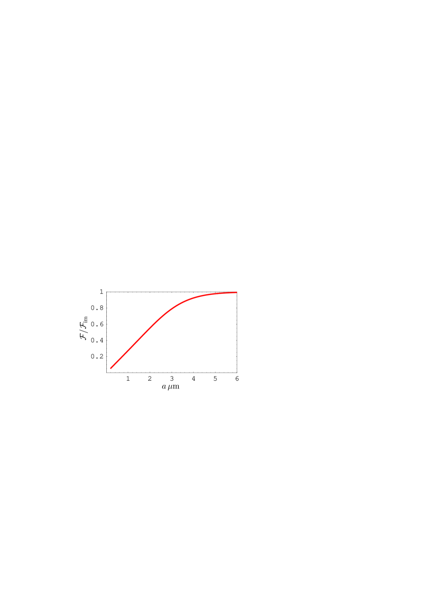
Figure 2: (Color online) The free energy of the Casimir-Polder interaction of an atom with graphene at $T=300\,$K normalized for the free energy of the same interaction with an ideal-metal plane is shown as a function of separation by the solid line.

In Ref. 45 it was found that at zero temperature the Casimir-Polder interaction between an atom and graphene is approximately 5% of the same interaction between an atom and an ideal metal plane. Here, we compare the Casimir-Polder interactions between an atom and graphene and between an atom and an ideal metal plane at room temperature. The solid line in Fig. 2 shows the ratio of atom-graphene free energy ${\cal F}$, computed using the exact expression for the polarization tensor with account of all contributing Matsubara frequencies in Ref. 44 , to the free energy ${\cal F}_{\rm im}$ of the same atom interacting with an ideal-metal plane. Both free energies are computed at $T=300\,$K as a function of separation in the region from 200 nm to $6\,\mu$m. Note that within the separation region considered only the static electric polarizability gives the dominant contribution to atom-graphene free energy. Because of this, we use the free energy of an atom-ideal plane interaction under the assumption that this atom is characterized by only the static electric polarizability $\alpha(0)$. This quantity is given by 11

$${\cal F}_{\rm im}(a,T)=-\frac{k_{B}T\alpha(0)}{4a^{3}}\left[1+\frac{2}{e^{\tau}-1}+\frac{2\tau e^{\tau}}{(e^{\tau}-1)^{2}}\right.$$

$$~{}~{}~{}~{}~{}~{}~{}~{}~{}~{}~{}~{}\left.+\frac{\tau^{2}e^{\tau}(e^{\tau}+1)}{(e^{\tau}-1)^{3}}\right],$$ (39)

where $\tau\equiv 4\pi ak_{B}T/(\hbar c)$. The value of $\Delta$ in the region from 0 to 0.1 eV influences the computational results for the free energy of atom-graphene interaction only in the fourth significant figure.

As can be seen in Fig. 2, at $a=200\,$nm the free energy of atom-graphene interaction is equal to approximately 5% of the free energy of atom interacting with ideal metal plane, as was found in Ref. 45 at zero temperature. However, with increasing separation the ratio ${\cal F}/{\cal F}_{\rm im}$ quickly increases. Thus, at separations 1 and $5\,\mu$m it is equal to 27% and 98%, respectively. At $a\geq 6\,\mu$m the Casimir-Polder free energy and force for atom-graphene interaction become equal to those for atom interacting with an ideal-metal plane. Because of this, the finding of Ref. 45 , where the 5% ratio was prolonged up to $5\,\mu$m, are applicable to only zero temperature and cannot be extrapolated to the case of room temperature.

In the end of this section we briefly discuss the impact of dynamic atomic polarizability and nonzero penetration depth of the electromagnetic oscillations into real metal on the conclusions obtained. If one considers an atom described by the dynamic electric polarizability and an Au plate characterized by the frequency-dependent dielectric permittivity, the magnitudes of the resulting Casimir-Polder free energy are equal 10 to $\approx 50$% and $\approx 90$% of the respective magnitudes calculated by using the static polarizability of an atom and an ideal-metal plane at separations 200 nm and $1\,\mu$m, respectively. Then one can conclude that the magnitudes of the Casimir-Polder free energy between a real atom and a graphene sheet are equal to approximately 10% and 30% of the magnitudes calculated for the same atom interacting with an Au plate at the same respective separations $a=200\,$nm and $a=1\,\mu$m.

V Microparticle interacting with thin film deposited on a substrate

Now we consider the classical Casimir-Polder interaction of an atom (microparticle) with thin material film of thickness $D$ deposited on thick substrate (semispace). We first assume that both the film and the substrate are made of magnetodielectric materials with finite $\varepsilon_{0}^{(1)}$ and $\varepsilon_{0}^{(2)}$ (see Fig. 1). From Eqs. (4) and (5) one obtains

$$r_{\rm TM}^{(0,1)}(0,y)=r_{\varepsilon}^{(1)},\quad r_{\rm TM}^{(1,2)}(0,y)=\frac{\varepsilon_{0}^{(2)}-\varepsilon_{0}^{(1)}}{\varepsilon_{0}^{(2)}+\varepsilon_{0}^{(1)}}\equiv r_{\varepsilon}^{(2,1)},$$ (40)

where $r_{\varepsilon}^{(1)}$ is defined in Eq. (6). Substituting Eq. (40) in Eq. (3) for $R_{\rm TM}$, we find

$$R_{\rm TM}(0,y)=\frac{r_{\varepsilon}^{(1)}+r_{\varepsilon}^{(2,1)}e^{-Dy/a}}{1+r_{\varepsilon}^{(1)}r_{\varepsilon}^{(2,1)}e^{-Dy/a}}\,.$$ (41)

Expanding here in powers of a small parameter $D/a$, we arrive at

$$R_{\rm TM}(0,y)\approx\frac{\varepsilon_{0}^{(2)}-1}{\varepsilon_{0}^{(2)}+1}-\frac{{\varepsilon_{0}^{(2)}}^{2}-{\varepsilon_{0}^{(1)}}^{2}}{\varepsilon_{0}^{(1)}(\varepsilon_{0}^{(2)}+1)^{2}}\,\frac{D}{a}\,y.$$ (42)

The respective result for $R_{\rm TE}(0,y)$ is obtained from Eq. (42) by the replacements $\varepsilon_{0}^{(1)}\to\mu_{0}^{(1)}$ and $\varepsilon_{0}^{(2)}\to\mu_{0}^{(2)}$.

Substituting $R_{\rm TM}$ from Eq. (42) and $R_{\rm TE}$ to Eq. (18), after the integration with respect to $y$ we obtain the classical Casimir-Polder free energy

$${\cal F}(a,T)\approx-\frac{k_{B}T}{4a^{3}}\left\{\alpha(0)\frac{\varepsilon_{0}^{(2)}-1}{\varepsilon_{0}^{(2)}+1}\left[1-3\frac{{\varepsilon_{0}^{(2)}}^{2}-{\varepsilon_{0}^{(1)}}^{2}}{\varepsilon_{0}^{(1)}({\varepsilon_{0}^{(2)}}^{2}-1)}\,\frac{D}{a}\right]\right.$$

$$~{}~{}~{}~{}~{}\left.+\beta(0)\frac{\mu_{0}^{(2)}-1}{\mu_{0}^{(2)}+1}\left[1-3\frac{{\mu_{0}^{(2)}}^{2}-{\mu_{0}^{(1)}}^{2}}{\mu_{0}^{(1)}({\mu_{0}^{(2)}}^{2}-1)}\,\frac{D}{a}\right]\right\}.$$ (43)

The respective classical Casimir-Polder force between a microparticle and thin material film deposited on a substrate is given by

$${F}(a,T)\approx-\frac{3k_{B}T}{4a^{4}}\left\{\alpha(0)\frac{\varepsilon_{0}^{(2)}-1}{\varepsilon_{0}^{(2)}+1}\left[1-4\frac{{\varepsilon_{0}^{(2)}}^{2}-{\varepsilon_{0}^{(1)}}^{2}}{\varepsilon_{0}^{(1)}({\varepsilon_{0}^{(2)}}^{2}-1)}\,\frac{D}{a}\right]\right.$$

$$~{}~{}~{}~{}~{}\left.+\beta(0)\frac{\mu_{0}^{(2)}-1}{\mu_{0}^{(2)}+1}\left[1-4\frac{{\mu_{0}^{(2)}}^{2}-{\mu_{0}^{(1)}}^{2}}{\mu_{0}^{(1)}({\mu_{0}^{(2)}}^{2}-1)}\,\frac{D}{a}\right]\right\}.$$ (44)

It is of interest to consider specific cases of Eqs. (43) and (44). Thus, for a nonmagnetic film ($\mu_{0}^{(1)}=1$) on a magnetic substrate we have from Eq. (43)

$${\cal F}(a,T)\approx-\frac{k_{B}T}{4a^{3}}\left\{\alpha(0)\frac{\varepsilon_{0}^{(2)}-1}{\varepsilon_{0}^{(2)}+1}\left[1-3\frac{{\varepsilon_{0}^{(2)}}^{2}-{\varepsilon_{0}^{(1)}}^{2}}{\varepsilon_{0}^{(1)}({\varepsilon_{0}^{(2)}}^{2}-1)}\,\frac{D}{a}\right]\right.$$

$$~{}~{}~{}~{}~{}\left.+\beta(0)\frac{\mu_{0}^{(2)}-1}{\mu_{0}^{(2)}+1}\left(1-3\frac{D}{a}\right)\right\},$$ (45)

i.e., the correction term does not depend on the magnetic permeability of the substrate $\mu_{0}^{(2)}$. Similar result holds also for the Casimir-Polder force. For an isolated film in a vacuum, i.e., for $\varepsilon_{0}^{(2)}=\mu_{0}^{(2)}=1$, Eqs. (43) and (44) coincide with Eqs. (10) and (11), respectively.

The next case to consider is the classical Casimir-Polder interaction between an atom (microparticle) and a dielectric film deposited on a metallic substrate (note that in the case of metallic film the role of substrate made of any material is negligibly small). We start from the contribution of the TM mode. Here the result does not depend on the used model of substrate metal. From Eqs. (4) and (5) one easily finds

$$r_{\rm TM}^{(0,1)}(0,y)=r_{\varepsilon}^{(1)},\quad r_{\rm TM}^{(1,2)}(0,y)=1.$$ (46)

Then from Eq. (3) we obtain

$$R_{\rm TM}(0,y)=\frac{r_{\varepsilon}^{(1)}+e^{-Dy/a}}{1+r_{\varepsilon}^{(1)}e^{-Dy/a}}\,.$$ (47)

Expanding in this equation in powers of the small parameter $D/a$, one arrives at

$$R_{\rm TM}(0,y)\approx 1-\frac{1}{\varepsilon_{0}^{(1)}}\,\frac{D}{a}\,y\,.$$ (48)

Substituting Eq. (48) in the first term on the right-hand side of Eq. (8) and integrating, one obtains the contribution of the TM mode to the classical Casimir-Polder free energy

$${\cal F}_{\rm TM}(a,T)\approx-\frac{k_{B}T\alpha(0)}{4a^{3}}\left(1-\frac{3}{\varepsilon_{0}^{(1)}}\,\frac{D}{a}\right).$$ (49)

The contribution of the TE mode depends on the model of substrate metal. We first assume that the low-frequency behavior of the dielectric permittivity of substrate metal is described by the Drude model. In this case the reflection coefficient $R_{\rm TE}(0,y)$ coincides with the same coefficient for an atom interacting with a dielectric film deposited on the dielectric substrate. The respective contribution to the Casimir-Polder free energy is given by the second term on the right-hand side of Eq. (43):

$${\cal F}_{\rm TE}(a,T)\approx-\frac{k_{B}T\beta(0)}{4a^{3}}\,\frac{\mu_{0}^{(2)}-1}{\mu_{0}^{(2)}+1}\left[1-3\frac{{\mu_{0}^{(2)}}^{2}-{\mu_{0}^{(1)}}^{2}}{\mu_{0}^{(1)}({\mu_{0}^{(2)}}^{2}-1)}\,\frac{D}{a}\right].$$ (50)

As a result, the total classical Casimir-Polder free energy and force in this case are given by

$${\cal F}_{D}(a,T)\approx-\frac{k_{B}T}{4a^{3}}\left\{\alpha(0)\left(1-\frac{3}{\varepsilon_{0}^{(1)}}\,\frac{D}{a}\right)\right.$$

$$~{}~{}~{}~{}\left.+\beta(0)\frac{\mu_{0}^{(2)}-1}{\mu_{0}^{(2)}+1}\left[1-3\frac{{\mu_{0}^{(2)}}^{2}-{\mu_{0}^{(1)}}^{2}}{\mu_{0}^{(1)}({\mu_{0}^{(2)}}^{2}-1)}\,\frac{D}{a}\right]\right\},$$

(51)

$${F}_{D}(a,T)\approx-\frac{3k_{B}T}{4a^{4}}\left\{\alpha(0)\left(1-\frac{4}{\varepsilon_{0}^{(1)}}\,\frac{D}{a}\right)\right.$$

$$~{}~{}~{}~{}\left.+\beta(0)\frac{\mu_{0}^{(2)}-1}{\mu_{0}^{(2)}+1}\left[1-4\frac{{\mu_{0}^{(2)}}^{2}-{\mu_{0}^{(1)}}^{2}}{\mu_{0}^{(1)}({\mu_{0}^{(2)}}^{2}-1)}\,\frac{D}{a}\right]\right\}.$$

For a nonmagnetic substrate these expressions are simplified. For example, the free energy takes the form

$${\cal F}_{D}(a,T)\approx-\frac{k_{B}T}{4a^{3}}\left[\vphantom{\frac{{\mu_{0}^{(1)}}^{2}-1}{\mu_{0}^{(1)}}}\alpha(0)\left(1-\frac{3}{\varepsilon_{0}^{(1)}}\,\frac{D}{a}\right)\right.$$ (52)

$$~{}~{}~{}~{}\left.+\beta(0)\frac{3}{4}\,\frac{{\mu_{0}^{(1)}}^{2}-1}{\mu_{0}^{(1)}}\,\frac{D}{a}\right].$$

Let us now assume that the metal of a substrate is described by the plasma model. In this case the contribution of the TM mode to the free energy is again given by Eq. (49). The TE reflection coefficients (4) are given by

$$r_{\rm TE}^{(0,1)}(0,y)=r_{\mu}^{(1)},$$ (53)

$$r_{\rm TE}^{(1,2)}(0,y)=\frac{\mu_{0}^{(2)}y-\mu_{0}^{(1)}\sqrt{y^{2}+\mu_{0}^{(2)}{\tilde{\omega}_{p}^{(2)}}{\vphantom{{\tilde{\omega}_{p}^{(2)}}}}^{2}}}{\mu_{0}^{(2)}y+\mu_{0}^{(1)}\sqrt{y^{2}+\mu_{0}^{(2)}{\tilde{\omega}_{p}^{(2)}}{\vphantom{{\tilde{\omega}_{p}^{(2)}}}}^{2}}}\,,$$

where the normalized plasma frequency of the substrate metal $\tilde{\omega}_{p}^{(2)}$ is defined in the same way as $\tilde{\omega}_{p}^{(1)}$ in Eq. (18) and expressed via the penetration depth $\delta^{(2)}$ of the electromagnetic oscillations into the material of a substrate. The coefficient $r_{\rm TE}^{(1,2)}$ in Eq. (53) can be identically presented as

$$r_{\rm TE}^{(1,2)}(0,y)=\frac{\frac{\delta^{(2)}}{2a}\,\frac{\sqrt{\mu_{0}^{(2)}}}{\mu_{0}^{(1)}}y-\left[1+\left(\frac{\delta^{(2)}}{2a}\right)^{2}\frac{y^{2}}{\mu_{0}^{(2)}}\right]^{1/2}}{\frac{\delta^{(2)}}{2a}\,\frac{\sqrt{\mu_{0}^{(2)}}}{\mu_{0}^{(1)}}y+\left[1+\left(\frac{\delta^{(2)}}{2a}\right)^{2}\frac{y^{2}}{\mu_{0}^{(2)}}\right]^{1/2}}.$$ (54)

Expanding Eq. (54) in powers of small parameter $\delta^{(2)}\sqrt{\mu_{0}^{(2)}}/(2a)$, we obtain

$$r_{\rm TE}^{(1,2)}(0,y)\approx-1+\frac{\delta^{(2)}}{a}\,\frac{\sqrt{\mu_{0}^{(2)}}}{\mu_{0}^{(1)}}y$$ (55)

in close analogy with Eq. (21).

Substituting Eq. (55) and the quantity $r_{\rm TE}^{(0,1)}$ from Eq. (53) in Eq. (3) and expanding in powers of small parameters $\delta^{(2)}\sqrt{\mu_{0}^{(2)}}/(2a)$ and $\mu_{0}^{(1)}D/a$, we find

$$R_{\rm TE}(0,y)\approx-1+\sqrt{\mu_{0}^{(2)}}\frac{\delta^{(2)}}{a}\,y+\mu_{0}^{(1)}\frac{D}{a}y.$$ (56)

Then from Eq. (8) one arrives to the following TE contribution to the Casimir-Polder free energy:

$${\cal F}_{\rm TE}(a,T)\approx\frac{k_{B}T}{4a^{3}}\beta(0)\left(1-3\sqrt{\mu_{0}^{(2)}}\frac{\delta^{(2)}}{a}\,-3\mu_{0}^{(1)}\frac{D}{a}\right).$$ (57)

Combining this with the TM contribution in Eq. (49), we obtain the Casimir-Polder free energy of an atom interacting with a dielectric film deposited on metallic substrate described by the plasma metal

$${\cal F}_{p}(a,T)\approx-\frac{k_{B}T}{4a^{3}}\left[\alpha(0)\left(1-\frac{3}{\varepsilon_{0}^{(1)}}\,\frac{D}{a}\right)\right.$$ (58)

$$-\left.\beta(0)\left(1-3\sqrt{\mu_{0}^{(2)}}\frac{\delta^{(2)}}{a}\,-3\mu_{0}^{(1)}\frac{D}{a}\right)\vphantom{\left(\frac{3}{\varepsilon_{0}^{(1)}}\right)}\right].$$

The respective expression for the Casimir-Polder force is

$${F}_{p}(a,T)\approx-\frac{3k_{B}T}{4a^{4}}\left[\alpha(0)\left(1-\frac{4}{\varepsilon_{0}^{(1)}}\,\frac{D}{a}\right)\right.$$ (59)

$$-\left.\beta(0)\left(1-4\sqrt{\mu_{0}^{(2)}}\frac{\delta^{(2)}}{a}\,-4\mu_{0}^{(1)}\frac{D}{a}\right)\vphantom{\left(\frac{3}{\varepsilon_{0}^{(1)}}\right)}\right].$$

From the comparison of Eq. (51) with Eq. (58) one can conclude that the contributions to the Casimir-Polder free energy due to atomic magnetic polarizability calculated using the Drude and plasma models are of opposite sign. The same is correct for the Casimir-Polder force, as it is seen from Eqs. (51) and (59).

VI Conclusions and discussion

In the foregoing we have derived simple analytic expressions for the classical Casimir-Polder free energy and force for a polarizable and magnetizable atom (microparticle) interacting with thin films made of dielectric and metallic magnetic materials, both isolated and deposited on substrates. The obtained results were compared with the Casimir-Polder interaction between an atom (microparticle) and a graphene sheet. It was shown that the classical Casimir-Polder interaction of an atom with a dielectric film is different from the same interaction of an atom with a dielectric plate (semispace). Specifically, it decreases quicker with separation and depends on an additional dimensional parameter, the film thickness.

The classical Casimir-Polder interaction of only electrically polarizable atoms with thin metallic films does not depend on the model of a metal and does not depend on film thickness. For magnetizable atoms (microparticles) the respective additions to the classical Casimir-Polder free energy and force depend on the film thickness when the film metal is magnetic and its low-frequency response is described by the Drude model. When the metal response is described by the plasma model, the additions due to atomic magnetic polarizability arise for both magnetic and nonmagnetic metals and depend on the penetration depth of electromagnetic oscillations into the metal. It the latter case the form of additions was shown to depend on the relationship between the film thickness, the penetration depth and the separation distance.

We have found analytic expressions for the Casimir-Polder free energy and force between a polarizable and magnetizable atom (microparticle) and a graphene sheet described by the polarization tensor in the framework of the Dirac model. It was shown that all contributions to these quantities due to atomic magnetic polarizability are suppressed, as compared to main terms depending on atomic electric polarizability. This conclusion is of interest for future experiments on quantum reflection and Bose-Einstein condensation near graphene surface. We have also shown that at room temperature the classical limit of the Casimir-Polder interaction with graphene is achieved at about $1.5\,\mu$m separation between an atom and a graphene surface. This is several times as big as for two graphene sheets, but several times as small as for two plates made of ordinary materials or for an atom above a plate. According to our results, at separations above $5\,\mu$m at $T=300\,$K the Casimir-Polder interaction of atoms with graphene is of the same strength as with an ideal-metal plane. This differs essentially from the previously investigated case of zero temperature where atom-graphene interaction was found to be as much as only 5% of the interaction of graphene with an ideal-metal plane. Qualitatively, the classical Casimir-Polder interaction of atoms with graphene was likened to the interaction with thin metallic film.

Finally, we have obtained simple analytic expressions for the Casimir-Polder interaction of an atom (microparticle) with thin magnetodielectric films deposited on both dielectric and metallic substrates made of magnetic or nonmagnetic materials. It was shown that in the case of magnetodielectric (dielectric) film deposited on metallic substrate the contributions to the Csimir-Polder free energy and force due to the magnetic atomic polarizability depend on the used model of metal. One can conclude that the classical Casimir-Polder interaction of atoms with thin films and graphene discussed above differs significantly from the interaction with thick cavity walls, and this might be interesting for future experiments on atom-surface interactions.

                 

Figure 1: The configuration of an atom (microparticle) above a thin film deposited on a thick substrate (semispace). See text for further discussion.

References

- (1) H. B. G. Casimir and D. Polder, Phys. Rev. 73, 360 (1948).
- (2) I. E. Dzyaloshinskii, E. M. Lifshitz, and L. P. Pitaevskii, Adv. Phys. 10, 165 (1961) [Usp. Fiz. Nauk 73, 381 (1961)].
- (3) Y. Tikochinsky and L. Spruch, Phys. Rev. A 48, 4236 (1993).
- (4) F. Shimizu, Phys. Rev. Lett. 86, 987 (2001).
- (5) H. Friedrich, G. Jacoby, and C. G. Meister, Phys. Rev. A 65, 032902 (2002).
- (6) V. Druzhinina and M. DeKieviet, Phys. Rev. Lett. 91, 193202 (2003).
- (7) D. M. Harber, J. M. McGuirk, J. M. Obrecht, and E. A. Cornell, J. Low. Temp. Phys. 133, 229 (2003).
- (8) A. E. Leanhardt, Y. Shin, A. P. Chikkatur, D. Kielpinski, W. Ketterle, and D. E. Pritchard, Phys. Rev. Lett. 90, 100404 (2003).
- (9) Y.-j. Lin, I. Teper, C. Chin, and V. Vuletić, Phys. Rev. Lett. 92, 050404 (2004).
- (10) J. F. Babb, G. L. Klimchitskaya, and V. M. Mostepanenko, Phys. Rev. A 70, 042901 (2004).
- (11) M. Antezza, L. P. Pitaevskii, and S. Stringari, Phys. Rev. A 70, 053619 (2004).
- (12) A. O. Caride, G. L. Klimchitskaya, V. M. Mostepanenko, and S. I. Zanette, Phys. Rev. A 71, 042901 (2005).
- (13) S. Y. Buhmann, L. Knöll, D.-G. Welsch, and H. T. Dung, Phys. Rev. A 70, 052117 (2004).
- (14) S. Y. Buhmann and D.-G. Welsch, Progr. Quant. Electronics 31, 51 (2007).
- (15) V. B. Bezerra, G. L. Klimchitskaya, V. M. Mostepanenko, and C. Romero, Phys. Rev. A 78, 042901 (2008).
- (16) J. M. Obrecht, R. J. Wild, M. Antezza, L. P. Pitaevskii, S. Stringari, and E. A. Cornell, Phys. Rev. Lett. 98, 063201 (2007).
- (17) V. B. Bezerra, G. L. Klimchitskaya, V. M. Mostepanenko, and C. Romero, Phys. Rev. D 81, 055003 (2010).
- (18) H. Safari, D.-G. Welsch, S. Y. Buhmann, and S. Scheel, Phys. Rev. A 78, 062109 (2008).
- (19) S. Y. Buhmann, H. Safari, H. T. Dung, and D.-G. Welsch, Opt. Spectrosc. 103, 374 (2007).
- (20) G. Bimonte, G. L. Klimchitskaya, and V. M. Mostepanenko, Phys. Rev. A 79, 042906 (2009).
- (21) Y. Roiter, M. Ornatska, A. R. Rammohan, J. Balakrishnan, D. R. Heine, and S. Minko, Nano Lett. 8, 941 (2008).
- (22) A. Canaguier-Durand, A. Gérardin, R. Guérout, P. A. Maia Neto, V. V. Nesvizhevsky, A. Yu. Voronin, A. Lambrecht, and S. Reynaud, Phys. Rev. A 83, 032508 (2011).
- (23) D. Kysylychyn, V. Piatnytsia, and V. Lozovski, Phys. Rev. E 88, 052403 (2013).
- (24) G. V. Dedkov and A. A. Kyasov, J. Comput. Theor. Nanosci. 10, 2342 (2013).
- (25) P.-O. Chapius, M. Laroche, S. Volz, and J.-J. Greffet, Phys. Rev. B 77, 125402 (2008).
- (26) A. H. Castro Neto, F. Guinea, N. M. R. Peres, K. S. Novoselov, and A. K. Geim, Rev. Mod. Phys. 81, 109 (2009).
- (27) M. S. Dresselhaus, Physica Status Solidi (b) 248, 1566 (2011).
- (28) A. Bogicevic, S. Ovesson, P. Hyldgaard, B. I. Lundqvist, H. Brune, and D. R. Jennison, Phys. Rev. Lett. 85, 1910 (2000).
- (29) E. Hult, P. Hyldgaard, J. Rossmeisl, and B. I. Lundqvist, Phys. Rev. B 64, 195414 (2001).
- (30) J. Jung, P. García-González, J. F. Dobson, and R. W. Godby, Phys. Rev. B 70, 205107 (2004).
- (31) J. F. Dobson, A. White, and A. Rubio, Phys. Rev. Lett. 96, 073201 (2006).
- (32) I. V. Bondarev and Ph. Lambin, Phys. Rev. B 70, 035407 (2004).
- (33) E. V. Blagov, G. L. Klimchitskaya, and V. M. Mostepanenko, Phys. Rev. B 71, 235401 (2005).
- (34) S. Y. Buhmann, S. Scheel, S. Å. Ellingsen, K. Hornberger, and A. Jacob, Phys. Rev. A 85, 042513 (2012).
- (35) M. Bordag, B. Geyer, G. L. Klimchitskaya, and V. M. Mostepanenko, Phys. Rev. B 74, 205431 (2006).
- (36) E. V. Blagov, G. L. Klimchitskaya, and V. M. Mostepanenko, Phys. Rev. B 75, 235413 (2007).
- (37) C. T. Weiß, P. V. Mironova, J. Fortágh, W. P. Schleich, and R. Walser, Phys. Rev. A 88, 043623 (2013).
- (38) A. D. Phan, T. X. Hoang, T. H. L. Nghiem, and L. M. Woods, Appl. Phys. Lett. 103, 163702 (2013).
- (39) M. Bordag, I. V. Fialkovsky, D. M. Gitman, and D. V. Vassilevich, Phys. Rev. B 80, 245406 (2009).
- (40) G. Gómez-Santos, Phys. Rev. B 80, 245424 (2009).
- (41) I. V. Fialkovsky, V. N. Marachevsky, and D. V. Vassilevich, Phys. Rev. B 84, 035446 (2011).
- (42) B. E. Sernelius, Phys. Rev. B 85, 195427 (2012).
- (43) M. Bordag, G. L. Klimchitskaya, and V. M. Mostepanenko, Phys. Rev. B 86, 165429 (2012).
- (44) G. L. Klimchitskaya and V. M. Mostepanenko, Phys. Rev. B 87, 075439 (2013).
- (45) Yu. V. Churkin, A. B. Fedortsov, G. L. Klimchitskaya, and V. A. Yurova, Phys. Rev. B 82, 165433 (2010).
- (46) T. E. Judd, R. G. Scott, A. M. Martin, B. Kaczmarek, and T. M. Fromhold, New. J. Phys. 13, 083020 (2011).
- (47) M. Chaichian, G. L. Klimchitskaya, V. M. Mostepanenko, and A. Tureanu, Phys. Rev. A 86, 012515 (2012).
- (48) S. Ribeiro and S. Scheel, Phys. Rev. A 88, 042519 (2013).
- (49) J. Feinberg, A. Mann, and M. Revzen, Ann. Phys. (N.Y.) 288, 103 (2001).
- (50) M. Bordag, G. L. Klimchitskaya, U. Mohideen, and V. M. Mostepanenko, Advances in the Casimir Effect (Oxford University Press, Oxford, 2009).
- (51) M. S. Tomaš, Phys. Lett. A 342, 381 (2005).
- (52) G. L. Klimchitskaya, U. Mohideen, and V. M. Mostepanenko, Rev. Mod. Phys. 81, 1827 (2009).
- (53) V. N. Marachevsky, Int. J. Mod. Phys.: Conf. Ser. 14, 435 (2012).