An efficient method for solving a correlated multi-item inventory system

Abstract

We propose an efficient method of finding an optimal solution for a multi-item continuous review inventory model in which a bivariate Gaussian probability distribution represents a correlation between the demands of different items. By utilizing appropriate normalizations of the demands, we show that the normalized demands are uncorrelated. Furthermore, the set of equations coupled with different items can be decoupled in such a way that the order quantity and reorder point for each item can be evaluated independently from those of the other. As a result, in contrast to conventional methods, the solution procedure for the proposed method can be much simpler and more accurate without any approximation. To demonstrate the advantage of the proposed method, we present a solution scheme for a multi-item continuous review inventory model in which the demand of optional components depend on that of a “vanilla box,” representing the customer’s stochastic demand, under stochastic payment and budget constraints. We also perform a sensitivity analysis to investigate the dependence of order quantities and reorder points on the correlation coefficient.

I Introduction

In a competitive global market, a manufacturer usually needs to provide a wide variety of products with a short amount of lead time to improve customer satisfaction and increase market share. When an order from a customer arrives, differentiation to the tailored order is often postponed down the assembly line to achieve both product variety and short lead time. In general, the more diverse a product, the longer lead time it requires. Modularization and postponement (or delayed differentiation) can be an effective means to reduce the lead time while maintaining a wide variety of products. Many modularization and postponement studies have shown that these concepts offer an advantage in terms of reducing uncertainty and forecasting errors with regard to demand (Ernst and Kamrad, 2000; Swaminathan and Tayur, 1998, 1999) in addition to creating product variety and customization at low cost (Chen et al., 2010). Thus, modularization and postponement have become important concepts in the market to provide better service to customers and make the business process more efficient.

In a product line such as computer retailing or automobile assembly, concepts of modularization and postponement are realized by an assembly process that consists of a semi-finished product “vanilla box” and optional components that are directly used in the final assembly. The vanilla box consists of components, known as the commonality of parts, needed to assemble the final product with appropriate optional components, and the vanilla box approach has been shown to be effective under high variance (Swaminathan and Tayur, 1998).

Applications of modularization and postponement to an inventory system require a multi-item model in which the demand of each of the several optional components depends on the demand or the presence of the vanilla box. The vanilla box represents the customer’s stochastic demand, and optional components, in turn, depend on the demand of the vanilla box for final assembly. Thus, the demands of the vanilla box and optional components are stochastically correlated. As the inventory model becomes complicated because of the correlation, it is desirable to find an efficient and accurate method to solve the model system.

A multi-item inventory model was proposed to comply with the concept of modularization and postponement (Wang and Hu, 2008). The model consists of a vanilla box and optional components in which the correlation between the two types of items is implemented as a bivariate Gaussian probability distribution whereas the optional components are independent of each other. This model handles a continuous review inventory system in which an order quantity $Q$ is placed whenever an inventory level reaches a certain reorder point $r$ under the presence of service level and budget constraints. Subsequently, a stochastic payment is also included in the model in such a manner that the total inventory cost does not exceed a predetermined budget (Wang and Hu, 2010).

In this paper, we propose an efficient method to solve a correlated multi-item continuous review inventory model in which the correlation between the vanilla box and an optional component is represented by a bivariate Gaussian probability distribution. By using appropriate normalizations of the demands of items, we show that the set of equations coupled with the vanilla box and optional components can be reduced to sets of decoupled equations for each item. Furthermore, each set of decoupled equations is simplified in a closed form and solved without any approximation. Thus, the equations for each item can be solved independently of each other.

The conventional method for solving such a model system is based on a heuristic of combining a Newton–Raphson method and a Hadley–Whitin iterative procedure (Wang and Hu, 2010). At each iteration, a candidate solution is found by using the Newton-Raphson method in which numerical integrations are carried out where required. The iteration proceeds until both $Q$ and $r$ sufficiently converge. Briefly, the conventional method takes the set of simultaneous equations for $Q$’s and $r$’s as a whole and utilizes heuristic approximating procedures. Given that the conventional method uses a rather complicated approximation and iteration, it requires heavy computation time.

In contrast, the proposed method does not rely on any approximation or heuristics. As a result, the solution procedure for the proposed method is much simpler, more accurate, and offers shorter computing time than the conventional method. We apply the proposed method to a correlated multi-item continuous review inventory model to demonstrate its usefulness. We also perform a sensitivity analysis in terms of the correlation to further characterize the behavior of the order quantity and reorder point of optional components. In addition, the proposed scheme can be used as a dependable method for a more generalized multi-item continuous review inventory model with much more complicated correlations among items.

The rest of this paper is organized as follows. Section II discusses the normalization of the demands and introduces an illustrative model to show how the set of simultaneous equations can be decoupled and simplified. Section III describes the proposed method for solving the model system. Section IV presents experimental results and discusses the sensitivity analysis. Section V summarizes the study and gives our conclusions.

II Normalization and multi-item inventory model

II.1 Correlation and normalization

Consider a multi-item inventory model that includes the correlation between a vanilla box and an optional component. Furthermore, we allow multiple optional components and each optional component is dependent on the vanilla box through a bivariate Gaussian probability distribution, whereas optional components are independent of each other.

A bivariate Gaussian probability distribution function (PDF) of the random variables $X_{v}$ and $X_{j}$ of the demand for the vanilla box and the $j$th optional component, respectively, is given by

$$f(x_{v},x_{j})=\frac{1}{2\pi\sqrt{|\Sigma|}}\exp\left\{-\frac{1}{2}(\vec{x}-\vec{\mu})^{T}\Sigma^{-1}(\vec{x}-\vec{\mu})\right\}~{}.$$ (1)

Here, the variable vector $\vec{x}$, the mean vector $\vec{\mu}$, the covariance matrix $\Sigma$, and the correlation coefficient $\rho_{j}$ between $X_{v}$ and $X_{j}$ are expressed, respectively, as

$$\vec{x}=\left[\begin{array}[]{c}x_{v}\\ x_{j}\end{array}\right],~{}\vec{\mu}=\left[\begin{array}[]{c}\mu_{v}\\ \mu_{j}\end{array}\right],~{}\Sigma=\left[\begin{array}[]{cc}\sigma_{v}^{2}&\sigma_{vj}\\ \sigma_{vj}&\sigma_{j}^{2}\end{array}\right],~{}\mbox{and}~{}\rho_{j}\equiv\frac{\sigma_{vj}}{\sigma_{v}\sigma_{j}}$$ (2)

with $|\Sigma|$ being the determinant of the $2\times 2$ matrix of $\Sigma$. Given that $X_{j}$ depends on $X_{v}$, we express the bivariate PDF as a product of the marginal PDF of $X_{v}$ and the conditional PDF of $X_{j}$ given $X_{v}=x_{v}$. In this way, the bivariate PDF of Eq. (1) can be written as

$$f(x_{v},x_{j}) = \frac{1}{\sqrt{2\pi}\sigma_{v}}\exp\left\{-\frac{(x_{v}-\mu_{v})^{2}}{2\sigma_{v}^{2}}\right\}\frac{1}{\sqrt{2\pi}\sigma_{j}\sqrt{1-\rho_{j}^{2}}}\exp\left\{-\frac{\left[x_{j}-\left(\mu_{j}+\rho_{j}\frac{\sigma_{j}}{\sigma_{v}}(x_{v}-\mu_{v})\right)\right]^{2}}{2\sigma_{j}^{2}(1-\rho_{j}^{2})}\right\}$$ (3)

$$\equiv f_{X_{v}}(x_{v})~{}f_{X_{j}|X_{v}}(x_{j}|x_{v})~{}.$$

In general, the demand for the vanilla box is equal to the customer’s demand, whereas the demand for each optional component depends on the safety stock of the vanilla box. Given that the safety stock of the vanilla box is $r_{v}-\mu_{v}$, the demand for each optional component depends on the reorder point of the vanilla box $r_{v}$. This implies that the conditional PDF of $X_{j}$ is evaluated at $X_{v}=r_{v}$. Motivated by this characteristic, we define the normalized random variables as

$$Z_{v}\equiv\frac{X_{v}-\mu_{v}}{\sigma_{v}}~{}~{}\mbox{and}~{}~{}Z_{j}\equiv\frac{X_{j}-\mu_{oj}}{\sigma_{oj}}~{},$$ (4)

where

$$\sigma_{oj}\equiv\sigma_{j}\sqrt{1-\rho_{j}^{2}}~{}~{}\mbox{and}~{}~{}\mu_{oj}\equiv\mu_{j}+\rho_{j}\frac{\sigma_{j}}{\sigma_{v}}(r_{v}-\mu_{v})~{}.$$ (5)

Note that the random variable $Z_{j}$ contains not only the demand $X_{j}$ of the $j$th optional component but also the reorder point $r_{v}$ of the vanilla box. With the normalization, the bivariate PDF at $X_{v}=r_{v}$ can be rewritten as

$$f_{X_{v}}(x_{v})~{}f_{X_{j}|X_{v}}(x_{j}|r_{v})=\frac{1}{\sqrt{2\pi}}e^{-z_{v}^{2}/2}\frac{1}{\sqrt{2\pi}}e^{-z_{j}^{2}/2}~{}.$$ (6)

We see from Eq. (6) that the normalization decomposes the bivariate PDF into a product of two PDFs of $Z_{v}$ and $Z_{j}$, both of which can be regarded as independent standard univariate PDFs. This implies that the notion of the conditional PDF does not exist and there is no distinction between dependent and independent items. In what follows, we take a correlated multi-item continuous review inventory system as an illustration of the advantage of normalization.

II.2 Model formulation and set of equations

The illustrative model we consider in this paper is a correlated multi-item continuous review inventory system that includes two types of items: a vanilla box and many optional components. Furthermore, as stated in Section II.1, each optional component depends on the vanilla box through a bivariate Gaussian probability distribution. We use the following notations to formulate the model:

• $A$ : fixed procuring cost,

• $C$ : unit variable procurement cost,

• $D$ : expected annual demand,

• $h$ : carrying cost,

• $p$ : unit shortage cost,

• $\kappa$ : service cost rate, and

• $\beta$ : available budget limit.

Note that each of these terms can be used for both the vanilla box and optional components whenever possible. We distinguish the vanilla box from the $j$th optional component by the subscripts $v$ and $oj$, respectively. For instance, $A_{v}$ and $A_{oj}$ represent the fixed procuring costs of the vanilla component and the $j$th optional component, respectively. The model is composed of the sum of the expected average annual cost (EAC) of the two types of items under budgetary constraint. The budgetary constraint, in turn, includes the service costs of the vanilla box and optional components. A detailed account of the model development can be found in (Wang and Hu, 2008, 2010).

The objective of the model is to minimize the sum of EAC for the vanilla box and $m$ optional components under a stochastic budgetary constraint. That is, we would like to find $(Q_{v},r_{v})$ and $(\vec{Q_{o}},\vec{r_{o}})$, where $\vec{Q_{o}}=(Q_{o1},Q_{o2},\cdots,Q_{om})$ and $\vec{r_{o}}=(r_{o1},r_{o2},\cdots,r_{om})$, that minimize

$$EAC(\vec{Q},\vec{r})=EAC_{1}(Q_{v},r_{v})+EAC_{2}(\vec{Q_{o}},\vec{r_{o}})$$ (7)

subject to

$$Prob\left\{C_{v}(Q_{v}+r_{v}-X_{v})+\sum_{j=1}^{m}C_{oj}(Q_{oj}+r_{oj}-X_{j})+\kappa_{v}F_{X_{v}}(r_{v})+\sum_{j=1}^{m}\kappa_{oj}F_{X_{j}|X_{v}}(r_{oj}|r_{v})\leq\beta\right\}\geq\eta$$ (8)

for

$$Q_{v}\geq 0,~{}r_{v}\geq 0~{}~{}\mbox{and}~{}~{}Q_{oj}\geq 0,~{}r_{oj}\geq 0~{}~{}\mbox{for}~{}~{}j=1,2,\cdots,m~{}.$$ (9)

In addition, $F_{X_{v}}(r_{v})$ and $F_{X_{j}|X_{v}}(r_{oj}|r_{v})$ are the cumulative density functions (CDFs) of $f_{X_{v}}(x_{v})$ and $f_{X_{j}|X_{v}}(x_{j}|x_{v})$, respectively. $EAC_{1}$ and $EAC_{2}$ are given as

$$EAC_{1}(Q_{v},r_{v}) = \frac{A_{v}D_{v}}{Q_{v}}+C_{v}D_{v}+h_{v}\left(\frac{Q_{v}}{2}+r_{v}-\mu_{v}\right)+\frac{p_{v}D_{v}}{Q_{v}}\int_{r_{v}}^{\infty}(x-r_{v})f_{X_{v}}(x)dx~{},$$ (10)

$$EAC_{2}(\vec{Q_{o}},\vec{r_{o}}) = \sum_{j=1}^{m}\left[\frac{A_{oj}D_{oj}}{Q_{oj}}+C_{oj}D_{oj}+h_{oj}\left(\frac{Q_{oj}}{2}+r_{oj}-\mu_{oj}\right)+\frac{p_{oj}D_{oj}}{Q_{oj}}\int_{r_{oj}}^{\infty}(x-r_{oj})f_{X_{j}|X_{v}}(x|r_{v})dx\right],$$ (11)

where $\mu_{oj}$ is defined as in Eq. (5). It is readily shown that the constraint of Eq. (8) can be rewritten as

$$C_{v}(Q_{v}+r_{v})+\sum_{j=1}^{m}C_{oj}(Q_{oj}+r_{oj})+\kappa_{v}F_{X_{v}}(r_{v})+\sum_{j=1}^{m}\kappa_{oj}F_{X_{j}|X_{v}}(r_{oj}|r_{v})\leq\beta+\mu_{Y}+z_{1-\eta}\sigma_{Y}~{},$$ (12)

where

$$\mu_{Y}\equiv C_{v}\mu_{v}+\sum_{j=1}^{m}C_{oj}\mu_{oj}~{},~{}~{}\sigma_{Y}^{2}\equiv C_{v}^{2}\sigma_{v}^{2}+\sum_{j=1}^{m}C_{oj}^{2}\sigma_{oj}^{2}~{},$$ (13)

and $z_{1-\eta}=F^{-1}(1-\eta)$ with $F^{-1}(1-\eta)$ being the inverse of the standard Gaussian CDF of the probability $\eta$.

With the model, the Lagrangian function $J$ using the Lagrangian relaxation can be written as

$$J = EAC_{1}(Q_{v},r_{v})+EAC_{2}(\vec{Q_{o}},\vec{r_{o}})+\lambda\left\{C_{v}(Q_{v}+r_{v})+\sum_{j=1}^{m}C_{oj}(Q_{oj}+r_{oj})\right.$$ (14)

$$\left.+\kappa_{v}F_{X_{v}}(r_{v})+\sum_{j=1}^{m}\kappa_{oj}F_{X_{j}|X_{v}}(r_{oj}|r_{v})-\left(\beta+\mu_{Y}+z_{1-\eta}\sigma_{Y}\right)\right\}~{}.$$

The first order necessary conditions can be achieved by differentiating $J$ with respect to $Q_{v}$, $r_{v}$, $Q_{oj}$, $r_{oj}$, and $\lambda$:

$$\frac{\partial J}{\partial Q_{oj}} = -\frac{A_{oj}D_{oj}}{Q_{oj}^{2}}+\frac{h_{oj}}{2}-\frac{p_{oj}D_{oj}}{Q_{oj}^{2}}\int_{r_{oj}}^{\infty}(x-r_{oj})f_{X_{j}|X_{v}}(x|r_{v})dx+\lambda C_{oj}=0$$ (15)

$$\frac{\partial J}{\partial r_{oj}} = h_{oj}+\frac{p_{oj}D_{oj}}{Q_{oj}}\frac{\partial}{\partial r_{oj}}\int_{r_{oj}}^{\infty}(x-r_{oj})f_{X_{j}|X_{v}}(x|r_{v})dx+\lambda C_{oj}+\lambda\kappa_{oj}\frac{\partial}{\partial r_{oj}}F_{X_{j}|X_{v}}(r_{oj}|r_{v})=0~{}~{}$$ (16)

$$\frac{\partial J}{\partial Q_{v}} = -\frac{A_{v}D_{v}}{Q_{v}^{2}}+\frac{h_{v}}{2}-\frac{p_{v}D_{v}}{Q_{v}^{2}}\int_{r_{v}}^{\infty}(x-r_{v})f_{X_{v}}(x)dx+\lambda C_{v}=0~{}~{}$$ (17)

$$\frac{\partial J}{\partial r_{v}} = h_{v}+\frac{p_{v}D_{v}}{Q_{v}}\frac{\partial}{\partial r_{v}}\int_{r_{v}}^{\infty}(x-r_{v})f_{X_{v}}(x)dx+\sum_{j=1}^{m}\frac{p_{oj}D_{oj}}{Q_{oj}}\int_{r_{oj}}^{\infty}(x-r_{oj})\frac{\partial}{\partial r_{v}}f_{X_{j}|X_{v}}(x|r_{v})dx$$ (18)

$$-\sum_{j=1}^{m}\left(h_{oj}+\lambda C_{oj}\right)\left(\rho_{j}\frac{\sigma_{j}}{\sigma_{v}}\right)+\lambda C_{v}+\lambda\kappa_{v}\frac{d}{dr_{v}}F_{X_{v}}(r_{v})+\sum_{j=1}^{m}\lambda\kappa_{oj}\frac{\partial}{\partial r_{v}}F_{X_{j}|X_{v}}(r_{oj}|r_{v})=0~{}~{}~{}$$

$$\frac{\partial J}{\partial\lambda} = C_{v}(Q_{v}+r_{v})+\sum_{j=1}^{m}\left[C_{oj}(Q_{oj}+r_{oj})\right]+\kappa_{v}F_{X_{v}}(r_{v})+\sum_{j=1}^{m}\kappa_{oj}F_{X_{j}|X_{v}}(r_{oj}|r_{v})-\left(\beta+\mu_{Y}+z_{1-\eta}\sigma_{Y}\right)=0.$$ (19)

Note that Eqs. (15)–(18) are simultaneous equations for $Q_{oj},r_{oj},Q_{v}$, and $r_{v}$.

II.3 Simplification of equations using normalization

Given that $Q_{oj}$ and $r_{oj}$ are coupled with $Q_{v}$ and $r_{v}$ from Eqs. (15)–(18), the equations are intractable to solve directly. For example, two equations [Eqs. (15) and (16)] contain three variables $Q_{oj}$, $r_{oj}$, and $r_{v}$. It turns out, however, that the normalizations discussed in Section II.1 can not only simplify the various expressions in Eqs. (15)–(18), but also, more importantly, decouple the equations for the optional components [Eqs. (15) and (16)] from the equations for the vanilla box [Eqs. (17) and (18)].

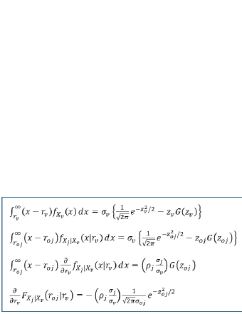
Figure 1: The list of expressions that are used to simplify the first order necessary condition.

Similarly to the normalization of Eq. (4), we further define the normalized reorder points as

$$z_{v}\equiv\frac{r_{v}-\mu_{v}}{\sigma_{v}}~{}~{}\mbox{and}~{}~{}z_{oj}\equiv\frac{r_{oj}-\mu_{oj}}{\sigma_{oj}}=\frac{(r_{oj}-\mu_{j})-\rho_{j}\frac{\sigma_{j}}{\sigma_{v}}(r_{v}-\mu_{v})}{\sigma_{j}\sqrt{1-\rho_{j}^{2}}}~{},$$ (20)

where we have used the definition of $\mu_{oj}$ of Eq. (5). Note that the normalized reorder point $z_{oj}$ is a function of $r_{oj}$ and $r_{v}$.

With the normalization defined in Eqs. (4) and (20), the various expressions in Eqs. (15)–(18) can be simplified as shown in Fig. 1. We derive the simplified expressions in detail in VI. With the normalization, Eqs. (15)–(19) can be re-expressed as

$$\frac{\partial J}{\partial Q_{oj}} = -\frac{A_{oj}D_{oj}}{Q_{oj}^{2}}+\frac{h_{oj}}{2}-\frac{p_{oj}D_{oj}}{Q_{oj}^{2}}\sigma_{oj}L(z_{oj})+\lambda C_{oj}=0$$ (21)

$$\frac{\partial J}{\partial r_{oj}} = h_{oj}-\frac{p_{oj}D_{oj}}{Q_{oj}}G(z_{oj})+\lambda C_{oj}+\lambda\frac{\kappa_{oj}}{\sigma_{oj}}f(z_{oj})=0$$ (22)

$$\frac{\partial J}{\partial Q_{v}} = -\frac{A_{v}D_{v}}{Q_{v}^{2}}+\frac{h_{v}}{2}-\frac{p_{v}D_{v}}{Q_{v}^{2}}\sigma_{v}L(z_{v})+\lambda C_{v}=0$$ (23)

$$\frac{\partial J}{\partial r_{v}} = h_{v}-\frac{p_{v}D_{v}}{Q_{v}}G(z_{v})+\lambda C_{v}+\lambda\frac{\kappa_{v}}{\sigma_{v}}f(z_{v})=0$$ (24)

$$\frac{\partial J}{\partial\lambda} = C_{v}\left(Q_{v}+\sigma_{v}z_{v}\right)+\sum_{j=0}^{m}C_{oj}\left(Q_{oj}+\sigma_{oj}z_{oj}\right)+\kappa_{v}F(z_{v})+\sum_{j=0}^{m}\kappa_{oj}F(z_{oj})$$ (25)

$$-\left(\beta+\mu_{Y}+z_{1-\eta}\sigma_{Y}\right)=0~{}.$$

Here, we define

$$f(z)\equiv\frac{1}{\sqrt{2\pi}}e^{-z^{2}/2}~{},~{}G(z)\equiv\int_{z}^{\infty}f(t)~{}dt~{},~{}F(z)\equiv 1-G(z)~{},~{}~{}\mbox{and}~{}~{}L(z)\equiv f(z)-zG(z)~{}.$$ (26)

Note that, owing to the normalization, Eqs. (15)–(18) are decoupled into two sets of equations: Eqs. (21) and (22) and Eqs. (23) and (24). Furthermore, each set of equations is identical and differs from the other only by the subscript. This implies that Eqs. (21) and (22) can be solved independently from Eqs. (23) and (24). This is expected because the PDF of the bivariate Gaussian distribution [Eq. (3)] can be expressed as the product of the PDF of the normalized variables $Z_{v}$ and $Z_{j}$ [Eq. (6)]. Thus, Eqs. (21) and (22) can be solved for $Q_{oj}$ and $z_{oj}$ directly. Similarly, Eqs. (23) and (24) can be solved for $Q_{v}$ and $z_{v}$. Once $z_{oj}$ and $z_{v}$ are found, we can use Eqs. (4) and (20) to get $r_{oj}$ and $r_{v}$. In the next section, we describe how to solve the set of Eqs. (21)–(24) under the constraint of Eq. (25).

III Proposed method to solve the model system

Similar to the approach by (Ghalebsaz-Jeddi et al., 2004), the proposed method to solve the model system consists of two parts. First, we regard Eqs. (21)–(24) as a subproblem for a given $\lambda$. Second, we repeatedly solve the subproblem until we find the solution $\lambda$ to Eq. (25).

III.1 Procedures for solving the subproblem

For a given $\lambda$, we regard Eqs. (21)–(24) as a subproblem and solve them for $Q_{oj}$, $z_{oj}$, $Q_{v}$, and $z_{v}$. The crucial point is that solving Eqs. (21) and (22) for $z_{oj}$ and $Q_{oj}$ is independent of solving Eqs. (23) and (24) for $z_{v}$ and $Q_{v}$, respectively. Given that $G(z_{oj})$ can be numerically evaluated for any $z_{oj}$, we note that Eqs. (21) and (22) are functions of $Q_{oj}$ and $z_{oj}$ only. By eliminating $Q_{oj}$ from Eqs. (21) and (22), we obtain an equation for $z_{oj}$. In particular, Eqs. (21) and (22) can be rewritten, respectively, in terms of $Q_{oj}$ as

$$Q_{oj}^{2}=\frac{A_{oj}D_{oj}+p_{oj}D_{oj}\sigma_{oj}L(z_{oj})}{h_{oj}/2+\lambda C_{oj}}~{}~{}\mbox{and}~{}~{}Q_{oj}=\frac{p_{oj}D_{oj}G(z_{oj})}{h_{oj}+\lambda C_{oj}+\lambda\left(\kappa_{oj}/\sigma_{oj}\right)f(z_{oj})}~{}.$$ (27)

We can eliminate $Q_{oj}$ from Eq. (27), resulting in an equation for $g_{oj}(z_{oj})$ in terms of $z_{oj}$ only:

$$g_{oj}(z_{oj})\equiv\frac{p_{oj}D_{oj}G(z_{oj})}{h_{oj}+\lambda C_{oj}+\lambda\left(\kappa_{oj}/\sigma_{oj}\right)f(z_{oj})}-\left\{\frac{A_{oj}D_{oj}+p_{oj}D_{oj}\sigma_{oj}L(z_{oj})}{h_{oj}/2+\lambda C_{oj}}\right\}^{1/2}=0~{}.$$ (28)

There exists a unique solution $z_{oj}=z_{oj}^{\ast}$ of Eq. (28) if the following three conditions are satisfied:

(a)

$g_{oj}(z_{oj})$ is a continuous function in $z_{oj}$.

(b)

$g_{oj}(z_{oj})$ is strictly monotonic in $z_{oj}$.

(c)

There exist two distinct values $z_{1}$ and $z_{2}$ such that $g_{oj}(z_{1})~{}g_{oj}(z_{2})<0$.

Condition (a) is immediately satisfied because $f(z_{oj})$, $G(z_{oj})$, and $L(z_{oj})$ are continuous in $z_{oj}$. The following theorem satisfies condition (b).

Theorem 1.

$g_{oj}(z_{oj})$ is strictly decreasing function in $z_{oj}$.

The proof is given in VII. Finally, condition (c) imposes a restriction on the values of the parameters. Given that $g_{oj}(z_{oj})$ is a continuous and strictly decreasing function in $z_{oj}$ from conditions (a) and (b), by assuming that $z_{oj}>0$, the following two inequalities should be satisfied to meet condition (c): $g_{oj}(0)>0$ and $g_{oj}(+\infty)<0$. It is easy to see that the condition $g_{oj}(+\infty)<0$ is satisfied by noting that $G(+\infty)=0$ and $0<L(+\infty)<\infty$. Therefore, the values of the parameters have to satisfy $g_{oj}(0)>0$. That is,

$$g_{oj}(0)=\frac{1}{2}\frac{p_{oj}D_{oj}}{h_{oj}+\lambda C_{oj}+\lambda\kappa_{oj}/(\sqrt{2\pi}\sigma_{oj})}-\left\{\frac{A_{oj}D_{oj}+p_{oj}D_{oj}\sigma_{oj}/\sqrt{2\pi}}{h_{oj}/2+\lambda C_{oj}}\right\}^{1/2}>0~{}.$$ (29)

The values of the parameters should satisfy this inequality for Eq. (28) to have a a unique solution.

Given that Eq. (28) is a function of $z_{oj}$ only, one can use a simple search technique, such as a bisection method (see, for instance, [(Kincaid and Cheney, 2002)]), to solve it at least numerically if not analytically. Once the solution $z_{oj}^{\ast}$ of $g_{oj}(z_{oj}^{\ast})=0$ is obtained, we can substitute it back into Eq. (27) to get $Q_{oj}^{\ast}$, the solution of $Q_{oj}$. We repeat the same procedure for $j=1,2,\cdots,m$ to obtain the normalized reorder point and order quantity for the optional components.

The normalized reorder point $z_{v}$ and order quantity $Q_{v}$ for the vanilla box can be obtained by applying a method similar to that used for the optional components. That is, Eqs. (23) and (24) can be rewritten respectively in terms of $Q_{oj}$ as

$$Q_{v}^{2}=\frac{A_{v}D_{v}+p_{v}D_{v}\sigma_{v}L(z_{v})}{h_{v}/2+\lambda C_{v}}~{}~{}\mbox{and}~{}~{}Q_{v}=\frac{p_{v}D_{v}G(z_{v})}{h_{v}+\lambda C_{v}+\lambda\left(\kappa_{v}/\sigma_{v}\right)f(z_{v})}~{}.$$ (30)

The existence of a unique solution $z_{v}^{\ast}$ of

$$g_{v}(z_{v})\equiv\frac{p_{v}D_{v}G(z_{v})}{h_{v}+\lambda C_{v}+\lambda\left(\kappa_{v}/\sigma_{v}\right)f(z_{v})}-\left\{\frac{A_{v}D_{v}+p_{v}D_{v}\sigma_{v}L(z_{v})}{h_{v}/2+\lambda C_{v}}\right\}^{1/2}=0~{}$$ (31)

can be proven in a similar fashion to the case for $z_{oj}^{\ast}$ of Eq. (28). Thus, we can solve numerically for $z_{v}=z_{v}^{\ast}$; subsequently, we can solve for $Q_{v}=Q_{v}^{\ast}$ by substituting $z_{v}^{\ast}$ into either Eq. (23) or (24).

III.2 Algorithm for solving the model system

The solution scheme for the subproblem discussed in Section III.1 reduces the set of Eqs. (21)–(25) to one equation [Eq. (32)] with one unknown $\lambda$, which is implicitly dependent on the variables:

$$g(\lambda)=C_{v}\left(Q_{v}+\sigma_{v}z_{v}\right)+\sum_{j=0}^{m}C_{oj}\left(Q_{oj}+\sigma_{oj}z_{oj}\right)+\kappa_{v}F(z_{v})+\sum_{j=0}^{m}\kappa_{oj}F(z_{oj})-\left(\beta+\mu_{Y}+z_{1-\eta}\sigma_{Y}\right)~{}.$$ (32)

If $g(\lambda)>0$, then the constraint is violated; otherwise (that is, $g(\lambda)\leq 0$), the constraint is satisfied. By using the Lagrangian relaxation (Ghalebsaz-Jeddi et al., 2004), the proposed algorithm to obtain the optimal reorder points and order quantities for the optional components and vanilla box [$r_{oj}$, $Q_{oj}$, $r_{v}$, $Q_{v}$] is as follows:

Step 1:

Find $\lambda_{1}$ and $\lambda_{2}$ such that $g(\lambda_{1})>0$ and $g(\lambda_{2})<0$.

Step 2:

For each $\lambda_{1}$ and $\lambda_{2}$, solve the subproblem as follows:

Step 2(a):

For $j=1$ to $m$, numerically solve Eq. (28) for $z_{oj}$ to obtain $z_{oj}^{\ast}$, and substitute $z_{oj}^{\ast}$ into Eq. (27) to get $Q_{oj}^{\ast}$.

Step 2(b):

Numerically solve Eq. (31) for $z_{v}$ to obtain $z_{v}^{\ast}$, and substitute $z_{v}^{\ast}$ into Eq. (30) to get $Q_{v}^{\ast}$.

Step 3:

Let $\lambda_{new}=(\lambda_{1}+\lambda_{2})/2$ and find $Q_{oj}^{\ast}$, $z_{oj}^{\ast}$, $Q_{v}^{\ast}$, and $z_{v}^{\ast}$ from Steps 2(a) and 2(b). If $g(\lambda_{new})>0$, then let $\lambda_{1}=\lambda_{new}$; otherwise let $\lambda_{2}=\lambda_{new}$.

Step 4:

Repeat Steps 2 and 3 until $\left|g(\lambda_{1})\right|<\epsilon$ or $\left|g(\lambda_{2})\right|<\epsilon$, where $\epsilon$ is a predetermined error.

Step 5:

Use Eq. (20) to get $r_{v}^{\ast}$ and $r_{oj}^{\ast}$ from $z_{v}^{\ast}$ and $z_{oj}^{\ast}$, respectively.

IV Experimental results and discussion

We illustrate the performance of the proposed method by an experiment that consists of one vanilla box and two optional components (i.e., $m=2$). The parameters for the vanilla box and two optional components are listed in Table 1. They are the same as the parameters used in (Wang and Hu, 2010) and $\epsilon=10^{-7}$. Table 2 lists the solution to the model for a given input from Table 1 together with the results of (Wang and Hu, 2010).

Table 1: Parameters for the vanilla box and the two optional components with $\eta=0.9031$ so that $z_{1-\eta}=-1.3$.

	$A_{v}$	$C_{v}$	$D_{v}$	$h_{v}$	$p_{v}$	$\kappa_{v}$	$\mu_{v}$	$\sigma_{v}$	$\beta$
Vanilla box	700	150	10,000	6	8	4000	300	40	150,000
Optional component	$A_{oj}$	$C_{oj}$	$D_{oj}$	$h_{oj}$	$p_{oj}$	$\kappa_{oj}$	$\mu_{j}$	$\sigma_{j}$	$\rho_{j}$
1	40	3	4000	0.7	1.0	200	100	15	0.5
2	20	2	6000	0.4	0.7	150	170	20	0.8

We also perform a sensitivity analysis of the order quantities and reorder points for the optional components with respect to the correlation coefficient. It should be noted that $Q_{v}$ and $r_{v}$ are independent of $\rho_{j}$ from Eqs. (30) and (31). For the sensitivity analysis, we first need to find the behavior of $z_{oj}$ as $\rho_{j}$ varies. Figure 2 shows that $z_{oj}$ is almost constant with respect to $\rho_{j}$ although $z_{o1}$ decreases slightly for large value of $\rho_{1}$. This implies that the normalized reorder points are insensitive to the correlation coefficient.

Figure 3 shows the behavior of order quantities $Q_{oj}$ of the optional components as the correlation coefficient $\rho_{j}$ varies. From the first equation in Eq. (27), we see that the dependence of $Q_{oj}$ on $\rho_{j}$ stems from $\sigma_{oj}L(z_{oj})$. Because $z_{oj}$ is more or less insensitive to $\rho_{j}$ [Fig. 2], so is $L(z_{oj})$. Thus, considering $\rho_{j}$ dependence only, we have

$$Q_{oj}\propto\sigma_{oj}\approx\sigma_{j}\sqrt{1-\rho_{j}^{2}}~{}.$$ (33)

This implies that $Q_{oj}$ decreases as the absolute value of $\rho_{j}$ increases and $Q_{oj}$ reaches its maximum when $\rho_{j}=0$ as shown in Fig. 3. The maximum of $Q_{oj}$ at $\rho_{j}=0$ can also be proved as follows. From the first equation in Eq. (27), it can be readily shown that

$$\frac{dQ_{oj}}{d\rho_{j}}=-\frac{p_{oj}D_{oj}}{\left\{h_{oj}+2\lambda C_{oj}\right\}}\left\{\frac{L(z_{oj})+z_{oj}G(z_{oj})}{Q_{oj}}\right\}\frac{\sigma_{j}^{2}}{\sigma_{oj}}\rho_{j}~{}.$$ (34)

Thus, $Q_{oj}$ is extreme when $\rho_{j}=0$. Furthermore,

$$\left.\frac{d^{2}Q_{oj}}{d\rho_{j}^{2}}\right|_{\rho_{j}=0}=-\frac{p_{oj}D_{oj}}{\left\{h_{oj}+2\lambda C_{oj}\right\}}\left\{\frac{L(z_{oj})+z_{oj}G(z_{oj})}{Q_{oj}}\right\}\sigma_{j}<0$$ (35)

implies that $Q_{oj}$ has its maximum when $\rho_{j}=0$.

Table 2: Solutions for $Q_{v}$, $r_{v}$, $Q_{oj}$, and $r_{oj}$, together with $\lambda$ and the total cost.

	$Q_{v}$	$r_{v}$	$Q_{o1}$	$r_{o1}$	$Q_{o2}$	$r_{o2}$	$\lambda$	$EAV(\vec{Q},\vec{r})$
Proposed method	860.8246	341.6691	580.8890	121.5989	648.4425	202.7676	0.045190	1,536,070
(Wang and Hu, 2010)	862.3301	340.3125	579.6005	122.7817	647.4532	203.3750	0.045044	1,536,061

Figure 2: Plots of the normalized reorder points $z_{oj}$ for the optional components versus the correlation coefficient $\rho_{j}$.

Figure 4 shows the behavior of reorder points $r_{oj}$ of the optional components as the correlation coefficient $\rho_{j}$ varies. Unlike the order quantity, $r_{oj}$ reaches its maximum at a positive value of $\rho_{oj}$. For the behavior of $r_{oj}$, we can rewrite Eq. (20) as follows:

$$r_{oj}=\mu_{j}+\rho_{j}\frac{\sigma_{j}}{\sigma_{v}}\left(r_{v}-\mu_{v}\right)+\sigma_{j}\sqrt{1-\rho_{j}^{2}}~{}z_{oj}~{}.$$ (36)

Because $z_{oj}$ is almost independent of $\rho_{j}$, as $\rho_{j}$ increases, the second term on the right-hand side of Eq. (36) also increases while the third term decreases. Thus, there is a trade-off between the second and the third terms, resulting in an optimum value of $r_{oj}$. Furthermore, the maximum $r_{oj}$ occurs when

$$\rho_{j}^{max}\approx\frac{r_{v}-\mu_{v}}{\sqrt{\sigma_{v}^{2}~{}z_{oj}^{2}+\sigma_{j}^{2}~{}(r_{v}-\mu_{v})^{2}}}~{}.$$ (37)

This implies that $\rho_{j}^{max}$ depends on the safety stock $r_{v}-\mu_{v}$ of the vanilla box. Given that the safety stock is a positive quantity, we have $0<\rho_{j}^{max}<1$ unlike the maximum of $Q_{oj}$.

Figure 3: Plots of the order quantities $Q_{oj}$ for the optional components versus the correlation coefficient $\rho_{j}$.

Figure 4: Plots of the reorder points $r_{o1}$ for optional component 1 versus the correlation coefficient $\rho_{1}$ while $\rho_{2}=0.5$. Inset: Same plot for optional component 2.

V Summary and conclusion

In this paper, we presented an efficient method for finding an optimal solution ($Q$, $r$) to a correlated multi-item continuous review inventory model in which a bivariate Gaussian probability distribution is used as a correlation between the vanilla box and an optional component. By normalizations of the random variables for the demands, we showed that the bivariate Gaussian PDF can be expressed as a product of two independent Gaussian PDFs, which implies that the normalized random variables are uncorrelated.

To demonstrate the usefulness of the normalization, we solved a multi-item continuous review inventory ($Q$, $r$) model in which the vanilla box and optional components are correlated under stochastic payment and budget constraints. With normalization, we showed that the set of equations coupled with the vanilla box and optional components was decoupled into sets of equations for the normalized quantities. Furthermore, each set of decoupled equations was reduced to a closed form and could be solved numerically without any approximation.

We also performed the sensitivity analysis in terms of the correlation. We found that the order quantity and the reorder point of optional components depended on the strength of the correlation as we expected. In particular, we showed that the order quantity of an optional component reached its maximum when there was no correlation between the vanilla box and the optional component. In addition, the reorder point of an optional component reached a maximum that depended on the safety stock of the vanilla box.

The proposed method can be used as a dependable method for a generalized multi-item continuous review inventory model with complicated interactions among items. It would be interesting to investigate how far the proposed method can be applied to other types of correlation, such as a multivariate Gaussian or other multivariate distributions.

VI Appendix I: Simplification of various functions

In this appendix, we show how to simplify the expressions in Eqs. (15)–(18). To this end, we define various normalized variables as follows:

$$z\equiv\frac{x-\mu_{v}}{\sigma_{v}}~{}~{}\mbox{and}~{}~{}z_{v}\equiv\frac{r_{v}-\mu_{v}}{\sigma_{v}}~{},$$ (A-1)

$$z_{j}\equiv\frac{x-\mu_{oj}}{\sigma_{oj}}~{}~{}\mbox{and}~{}~{}z_{oj}\equiv\frac{r_{oj}-\mu_{oj}}{\sigma_{oj}}~{},$$ (A-2)

where

$$\sigma_{oj}\equiv\sigma_{j}\sqrt{1-\rho_{j}^{2}}~{}~{}\mbox{and}~{}~{}\mu_{oj}\equiv\mu_{j}+\rho_{j}\frac{\sigma_{j}}{\sigma_{v}}(r_{v}-\mu_{v})~{}.$$ (A-3)

In addition, from Eq. (3), we have

$$f_{X_{v}}(x)=\frac{1}{\sqrt{2\pi}\sigma_{v}}\exp\left\{-\frac{(x-\mu_{v})^{2}}{2\sigma_{v}^{2}}\right\}~{}~{}\mbox{and}~{}~{}f_{X_{j}|X_{v}}(x|r_{v})=\frac{1}{\sqrt{2\pi}\sigma_{oj}}\exp\left\{-\frac{(x-\mu_{oj})^{2}}{2\sigma_{oj}^{2}}\right\}~{}.$$ (A-4)

Finally, the G-function is defined as

$$G(z)\equiv\int_{z}^{\infty}\frac{1}{\sqrt{2\pi}}e^{-z^{2}/2}dz~{}.$$ (A-5)

VI.1 Evaluation of $\int_{r_{v}}^{\infty}(x-r_{v})f_{X_{v}}(x)dx$ and $\frac{d}{dr_{v}}\int_{r_{v}}^{\infty}(x-r_{v})f_{X_{v}}(x)dx$

From Eqs. (A-1) and (A-4), we have

$$\int_{r_{v}}^{\infty}(x-r_{v})f_{X_{v}}(x)dx=\frac{\sigma_{v}}{\sqrt{2\pi}}\int_{z_{v}}^{\infty}(z-z_{v})e^{-z^{2}/2}dz=\sigma_{v}\left\{\frac{1}{\sqrt{2\pi}}e^{-z_{v}^{2}/2}-z_{v}G(z_{v})\right\}~{}.$$ (A-6)

By using the above result, its derivative becomes

$$\frac{d}{dr_{v}}\int_{r_{v}}^{\infty}(x-r_{v})f_{X_{v}}(x)dx=\sigma_{v}\ \frac{dz_{v}}{dr_{v}}\frac{d}{dz_{v}}\left\{\frac{1}{\sqrt{2\pi}}e^{-z_{v}^{2}/2}-z_{v}G(z_{v})\right\}=-G(z_{v})~{}.$$ (A-7)

VI.2 Evaluation of $\int_{r_{oj}}^{\infty}(x-r_{oj})f_{X_{j}|X_{v}}(x|r_{v})dx$ and $\frac{\partial}{\partial r_{oj}}\int_{r_{oj}}^{\infty}(x-r_{oj})f_{X_{j}|X_{v}}(x|r_{v})dx$

From Eqs. (A-2)–(A-4), we have

$$\int_{r_{oj}}^{\infty}(x-r_{oj})f_{X_{j}|X_{v}}(x|r_{v})dx=\int_{r_{oj}}^{\infty}(x-r_{oj})\frac{1}{\sqrt{2\pi}\sigma_{oj}}\exp\left\{-\frac{(x-\mu_{oj})^{2}}{2\sigma_{oj}^{2}}\right\}dx$$ (A-8)

$$= \sigma_{j}\sqrt{1-\rho_{j}^{2}}\int_{z_{oj}}^{\infty}(z_{j}-z_{oj})\frac{1}{\sqrt{2\pi}}e^{-z_{j}^{2}/2}dz_{j}=\sigma_{oj}\left\{\frac{1}{\sqrt{2\pi}}e^{-z_{oj}^{2}/2}-z_{oj}G(z_{oj})\right\}~{}.$$

By using the above result, its derivative becomes

$$\frac{\partial}{\partial r_{oj}}\int_{r_{oj}}^{\infty}(x-r_{oj})f_{X_{j}|X_{v}}(x|r_{v})dx=\sigma_{oj}\frac{dz_{oj}}{dr_{oj}}\frac{\partial}{\partial z_{oj}}\left\{\frac{1}{\sqrt{2\pi}}e^{-z_{oj}^{2}/2}-z_{oj}G(z_{oj})\right\}=-G(z_{oj})~{}.$$ (A-9)

VI.3 Evaluation of $\int_{r_{oj}}^{\infty}(x-r_{oj})\frac{\partial}{\partial r_{v}}f_{X_{j}|X_{v}}(x|r_{v})dx$

By using Eq. (A-4), the partial derivative becomes

$$\frac{\partial}{\partial r_{v}}f_{X_{j}|X_{v}}(x|r_{v})=\frac{d\mu_{oj}}{dr_{v}}\frac{\partial}{\partial\mu_{oj}}\frac{1}{\sqrt{2\pi}\sigma_{oj}}\exp\left\{-\frac{(x-\mu_{oj})^{2}}{2\sigma_{oj}^{2}}\right\}=\left(\rho_{j}\frac{\sigma_{j}}{\sigma_{v}}\right)\frac{(x-\mu_{oj})}{\sqrt{2\pi}\sigma_{oj}^{3}}\exp\left\{-\frac{(x-\mu_{oj})^{2}}{2\sigma_{oj}^{2}}\right\}~{}.$$

Thus, by using Eqs. (A-2) and (A-4), we have

$$\int_{r_{oj}}^{\infty}(x-r_{oj})\frac{\partial}{\partial r_{v}}f_{X_{j}|X_{v}}(x|r_{v})dx=\left(\rho_{j}\frac{\sigma_{j}}{\sigma_{v}}\right)\int_{r_{oj}}^{\infty}(x-r_{oj})\frac{(x-\mu_{oj})}{\sqrt{2\pi}\sigma_{oj}^{3}}\exp\left\{-\frac{(x-\mu_{oj})^{2}}{2\sigma_{oj}^{2}}\right\}dx$$ (A-10)

$$= \left(\rho_{j}\frac{\sigma_{j}}{\sigma_{v}}\right)\int_{z_{oj}}^{\infty}(z_{j}-z_{oj})~{}z_{j}\frac{1}{\sqrt{2\pi}}e^{-z_{j}^{2}/2}dz_{j}=\left(\rho_{j}\frac{\sigma_{j}}{\sigma_{v}}\right)G(z_{oj})~{}.$$

VI.4 Evaluation of $\frac{d}{dr_{v}}F_{X_{v}}(r_{v})$, $\frac{\partial}{\partial r_{v}}F_{X_{j}|X_{v}}(r_{oj}|r_{v})$, and $\frac{\partial}{\partial r_{oj}}F_{X_{j}|X_{v}}(r_{oj}|r_{v})$

By using Eqs. (A-1) and (A-4), we have

$$F_{X_{v}}(r_{v})=\int_{-\infty}^{r_{v}}\frac{1}{\sqrt{2\pi}\sigma_{v}}\exp\left\{-\frac{(x-\mu_{v})^{2}}{2\sigma_{v}^{2}}\right\}dx=\int_{-\infty}^{z_{v}}\frac{1}{\sqrt{2\pi}}e^{-z^{2}/2}dz~{}.$$

Thus,

$$\frac{d}{dr_{v}}F_{X}(r_{v})=\frac{dz_{v}}{dr_{v}}\frac{d}{dz_{v}}\int_{-\infty}^{z_{v}}\frac{1}{\sqrt{2\pi}}e^{-z^{2}/2}dz=\frac{1}{\sqrt{2\pi}\sigma_{v}}e^{-z_{v}^{2}/2}~{}.$$ (A-11)

Similarly, by using Eqs. (A-2)–(A-4), we have

$$F_{X_{j}|X_{v}}(r_{oj}|r_{v})=\int_{-\infty}^{r_{oj}}\frac{1}{\sqrt{2\pi}\sigma_{oj}}\exp\left\{-\frac{(x-\mu_{oj})^{2}}{2\sigma_{oj}^{2}}\right\}dx=\int_{-\infty}^{z_{oj}}\frac{1}{\sqrt{2\pi}}e^{-z_{j}^{2}/2}dz_{j}~{}.$$

Thus,

$$\frac{\partial}{\partial r_{v}}F_{X_{j}|X_{v}}(r_{oj}|r_{v})=\frac{dz_{oj}}{dr_{v}}\frac{\partial}{\partial z_{oj}}\int_{-\infty}^{z_{oj}}\frac{1}{\sqrt{2\pi}}e^{-z_{j}^{2}/2}~{}dz_{j}=-\left(\rho_{j}\frac{\sigma_{j}}{\sigma_{v}}\right)\frac{1}{\sqrt{2\pi}\sigma_{oj}}e^{-z_{oj}^{2}/2}~{}.$$ (A-12)

Finally, by using Eqs. (A-2) and (A-4), we have

$$\frac{\partial}{\partial r_{oj}}F_{X_{j}|X_{v}}(r_{oj}|r_{v})=\frac{dz_{oj}}{dr_{oj}}\frac{\partial}{\partial z_{oj}}\int_{-\infty}^{z_{oj}}\frac{1}{\sqrt{2\pi}}e^{-z_{j}^{2}/2}~{}dz_{j}=\frac{1}{\sqrt{2\pi}\sigma_{oj}}e^{-z_{oj}^{2}/2}~{}.$$ (A-13)

VII Appendix II: Proof of Theorem 1

For brevity, we drop the subscript $oj$ for the optional component and assume $\lambda>0$. To prove that $g(z)$ of Eq. (28) is monotonically decreasing in $z$, it suffices to show that for any two values of $z$ such that $z_{1}<z_{2}$, $g(z)$ satisfies $g(z_{1})>g(z_{2})$. We start with

$$g(z)\equiv\frac{pDG(z)}{h+\lambda C+\lambda\kappa/\sigma f(z)}-\left\{\frac{AD+pD\sigma L(z)}{h/2+\lambda C}\right\}^{1/2}~{},$$ (B-1)

where the loss function $L(z)$, the standard Gaussian PDF $f(z)$, and $G(z)$ are defined, respectively, as

$$L(z)\equiv\sigma\left\{\frac{1}{\sqrt{2\pi}}e^{-z^{2}/2}-zG(z)\right\}~{},~{}~{}f(z)\equiv\frac{1}{\sqrt{2\pi}}e^{-z^{2}/2}~{},~{}~{}\mbox{and}~{}~{}G(z)\equiv\frac{1}{\sqrt{2\pi}}\int_{z}^{\infty}e^{-t^{2}/2}~{}dt~{}.$$

From Eq. (B-1), we have

$$g(z_{1})-g(z_{2})=\left\{\frac{pDG(z_{1})}{h+\lambda C+\lambda\kappa/\sigma f(z_{1})}-\frac{pDG(z_{2})}{h+\lambda C+\lambda\kappa/\sigma f(z_{2})}\right\}+\sqrt{\frac{pD\sigma}{h/2+\lambda C}}\sqrt{L(z_{2})-L(z_{1})}~{}.$$ (B-2)

Since $L(z_{1})<L(z_{2})$ for $z_{1}<z_{2}$, the second term on the right hand side of Eq. (B-2) is positive. The first term can be rewritten as

$$\left\{\frac{pDG(z_{1})}{h+\lambda C+\lambda\kappa/\sigma f(z_{1})}-\frac{pDG(z_{2})}{h+\lambda C+\lambda\kappa/\sigma f(z_{2})}\right\}$$ (B-3)

$$= pD\left\{\frac{(h+\lambda C)\left\{G(z_{1})-G(z_{2})\right\}+\lambda\kappa/\sigma\left\{G(z_{1})f(z_{2})-G(z_{2})f(z_{1})\right\}}{\left\{h+\lambda C+\lambda\kappa/\sigma f(z_{1})\right\}\left\{h+\lambda C+\lambda\kappa/\sigma f(z_{2})\right\}}\right\}~{}.$$

From the definition of $G(z)$, we have $G(z_{1})>G(z_{2})$ when $z_{1}<z_{2}$. Thus, to show that $g(z_{1})>g(z_{2})$ when $z_{1}<z_{2}$, we are left with showing that $G(z_{1})f(z_{2})-G(z_{2})f(z_{1})$ is positive.

To this end, consider the following expression:

$$h(z_{1})-h(z_{2})\equiv\frac{G(z_{1})f(z_{2})-G(z_{2})f(z_{1})}{f(z_{1})f(z_{2})}=\frac{G(z_{1})}{f(z_{1})}-\frac{G(z_{2})}{f(z_{2})}~{}.$$ (B-4)

Given that $f(z)>0$, to show $g(z_{1})>g(z_{2})$ when $z_{1}<z_{2}$ is equivalent to proving that $h(z_{1})>h(z_{2})$ when $z_{1}<z_{2}$. That is, $h(z)$ is a monotonically decreasing in $z$. Now, we express $G(z)/f(z)$ in terms of an infinite series in $z$ by using (Abramowitz and Stegun, 1972)

$$h(z)\equiv\frac{G(z)}{f(z)}=\sum_{n=0}^{\infty}(-1)^{n}\frac{(2n-1)!!}{z^{2n+1}}>0~{},$$ (B-5)

where

$$(2n-1)!!\equiv 1\cdot 3\cdot 5\cdots(2n-3)\cdot(2n-1)~{}.$$

By letting $m=n-1$, $h(z)$ can be rewritten as

$$h(z) = \sum_{n=0}^{\infty}(-1)^{n}\frac{(2n-1)!!}{z^{2n+1}}=\frac{1}{z}+\sum_{n=1}^{\infty}(-1)^{n}\frac{(2n-1)!!}{z^{2n+1}}$$ (B-6)

$$= \frac{1}{z}+\sum_{m=0}^{\infty}(-1)^{m+1}\frac{(2m+1)!!}{z^{2m+3}}=\frac{1}{z}-\sum_{m=0}^{\infty}(-1)^{m}\frac{(2m+1)!!}{z^{2m+3}}>0~{}.$$

Since $h(z)>0$ for all $z$, we have, from Eq. (B-6),

$$\sum_{m=0}^{\infty}(-1)^{m}\frac{(2m+1)!!}{z^{2m+3}}<\frac{1}{z}~{}.$$ (B-7)

To show that $h(z)$ is monotonically decreasing in $z$, we will show that $dh(z)/dz<0$. From Eq. (B-5), the derivative becomes

$$\frac{dh(z)}{dz}=\sum_{n=0}^{\infty}(-1)^{n}(2n-1)!!(-1)\frac{(2n+1)}{z^{2n+2}}=(-z)\sum_{n=0}^{\infty}(-1)^{n}\frac{(2n+1)!!}{z^{2n+3}}~{}.$$ (B-8)

By using Eq. (B-7), $dh(z)/dz$ can be expressed as

$$\frac{dh(z)}{dz}=(-z)\sum_{n=0}^{\infty}(-1)^{n}\frac{(2n+1)!!}{z^{2n+3}}<(-z)\frac{1}{z}<-1~{}.$$ (B-9)

Since $dh(z)/dz<0$ for all $z$, we have $h(z_{2})<h(z_{1})$ when $z_{2}>z_{1}$ . That is,

$$h(z_{1})-h(z_{2})\equiv\frac{G(z_{1})}{f(z_{1})}-\frac{G(z_{2})}{f(z_{2})}=\frac{G(z_{1})f(z_{2})-G(z_{2})f(z_{1})}{f(z_{1})f_{z_{2}}}>0~{}.$$ (B-10)

This completes the proof.

References

- Abdel-Malek and Areeratchakul (2007) Abdel-Malek L, Areeratchakul N (2007) A quadratic programming approach to the multi-product newsvendor problem with side constraints Euro. J. of Oper. Res. 176:1607–1619.
- Abramowitz and Stegun (1972) Abramowitz M, Stegun I, eds. (1972) Handbook of Mathematical Functions, (Dover, New York, 1972) p. 932.
- Byrkett (1981) Byrkett D (1981) An Empirical Evaluation of Further Approximations to An Approximate Continuous Review Inventory Model Naval Research Logistics Quarterly 28:169–180.
- Chen and Beaulieu (2009) Chen Y, Beaulieu N (2009) A simple polynomial approximation to the Gaussian Q-function and its application IEEE Communication Letters 13:124–126.
- Chen et al. (2010) Tze-Ming Chen, Tai-Yue Wang, Jui-Ming Hu, Optimal ordering policy in simple inventory models with modularization and postponement, Computers and Industrial Engineering (CIE), 2010 40th International Conference on, 25-28 July 2010, pp.1-14
- Das (1975) Das C (1975) Some Aids for Lot-Size Inventory Control under Normal Lead Time Demand AIEE Transactions 7:77–79.
- Das (1985) Das C (1985) On the Solution of Some Approximate Continuous Review Inventory Models Naval Research Logistics Quarterly 32:301–313.
- Ernst and Kamrad (2000) Ernst R, Kamrad, B (2000) Evaluation of supply chain structures through modularization and postponement Euro. J. of Oper. Res. 124:495–510.
- Ghalebsaz-Jeddi et al. (2004) Ghalebsaz-Jeddi B, Shultes B, Haji R (2004) A multi-product continuous review inventory system with stochastic demand, backorders, and a budget constraint Euro. J. of Oper. Res. 158:456–469.
- Herron (1967) Herron D (1967) Inventory Management for Minimum Cost Management Science 14:B219–235.
- Kincaid and Cheney (2002) Kincaid D, Cheney W (2002) Numerical Analysis: Mathematics of scientific computing, (Brooks/Cole, Pacific Grove, 2002).
- Kundu and Charkrabarti (2012) Kundu A, Charkrabarti T (2012) A multi-product continuous review inventory system in stochastic environment with budget constraint Optim. Lett 6:299–313.
- Swaminathan and Tayur (1998) Swaminathan JM, Tayur S (1998) Managing broader product lines through delayed differentiation using vanilla boxes. Management Science 44:S161–S172.
- Swaminathan and Tayur (1999) Swaminathan JM, Tayur S (1999) Managing design of assembly sequences for product lines that delay product differentiation. IIE Transactions 31:1015–1027.
- Wang and Hu (2008) Wang T, Hu J (2008) An inventory control system for products with optional components under service level and budget constraints. Euro. J. of Oper. Res. 189:41-58.
- Wang and Hu (2010) Wang T, Hu J (2010) Heuristic method on solving an inventory model for products with optional components under stochastic payment and budget constraints, Exp. Sys. with App. 37:2588–2598.