Axisymmetric equilibrium models for magnetized neutron stars in General Relativity under the Conformally Flat Condition

Abstract

Extremely magnetized neutron stars with magnetic fields as strong as $\sim 10^{15-16}$ G, or magnetars, have received considerable attention in the last decade due to their identification as a plausible source for Soft Gamma Repeaters and Anomalous X-ray Pulsars. Moreover, this class of compact objects has been proposed as a possible engine capable of powering both Long and Short Gamma-Ray Bursts, if the rotation period in their formation stage is short enough ($\sim 1$ ms). Such strong fields are expected to induce substantial deformations of the star and thus to produce the emission of gravitational waves. Here we investigate, by means of numerical modeling, axisymmetric static equilibria of polytropic and strongly magnetized stars in full general relativity, within the ideal magneto-hydrodynamic regime. The eXtended Conformally Flat Condition (XCFC) for the metric is assumed, allowing us to employ the techniques introduced for the X-ECHO code [Bucciantini & Del Zanna, 2011, Astron. Astrophys. 528, A101], proven to be accurate, efficient, and stable. The updated XNS code for magnetized neutron star equilibria is made publicly available for the community (see www.arcetri.astro.it/science/ahead/XNS). Several sequences of models are here retrieved, from the purely toroidal (resolving a controversy in the literature) or poloidal cases, to the so-called twisted torus mixed configurations, expected to be dynamically stable, which are solved for the first time in the non-perturbative regime.

1 Introduction

Neutron Stars (NSs) are the most compact objects in the universe endowed with an internal structure. Proposed originally by Baade & Zwicky (1934) in the context of supernova explosions, they were discovered only in 1967 by Hewish et al. (1968) as radio pulsars. Today, NSs are among the most studied objects in high-energy astrophysics because they are known to power many astrophysical sources of high energy emission. The extreme conditions characterizing their interior make them also interesting objects from the point of view of nuclear and condense matter physics, and future combined observations of both mass and radius of such compact objects may finally discriminate on the different equations of state (EoS) so far proposed (Feroci et al., 2012).

It was immediately evident that NSs can also harbour very high magnetic fields, usually inferred to be in the range $10^{8-12}$ G for normal pulsars. It is indeed this very strong magnetic field that is responsible for most of their phenomenology and emission. The amplification of magnetic fields form the initial values prior to collapse to those enhanced values is believed to take place during the formation of the compact object itself: surely due to the compression associated with the collapse of the core of the progenitor star (Spruit, 2009), it can be further increased by differential rotation in the core leading to the twisting of fieldlines (Burrows et al., 2007), and to possible dynamo effects (Bonanno, Rezzolla & Urpin, 2003; Rheinhardt & Geppert, 2005). In principle there is a large store of free energy available during and immediately following the collapse of the core and the formation of a proto-NS, such that a magnetic field as high as $10^{17-18}$ G could be even reached.

The magnetar model for Anomalous X-Ray Pulsars and Soft Gamma Repeaters (Thompson & Duncan, 1996; Mereghetti, 2008) suggests that the magnetic field can reach at least values close to $10^{16}$ G at the surface of NSs. Accounting also for the effects of dissipative processes (Viganò et al., 2013), given the typical ages of known magnetars ($\sim 10^{4}$ yr), it is not unreasonable to expect that younger magnetars with even higher magnetic fields might exist, and more so immediately after collapse and formation, due to the processes discussed above.

Magnetars could be fundamental also to explain another class of objects typical of high-energy astrophysics, namely Gamma Ray Bursts (GRBs). The combination of a rapid millisecond-like rotation of a compact NS with a magnetic field of typical magnetar strength, can easily drive a relativistic outflow with energetics of the order of $\sim 10^{49-50}$ erg s^-1, enough to power a classical Long GRB. Short GRBs have been instead usually associated to merger events, rather than to core collapse of stellar objects, leading to the formation of a rotating Black Hole (BH), similarly to the collapsar scenario for Long GRBs (Woosley, 1993; MacFadyen & Woosley, 1999). However, the recent discovery, on the one hand of extended emission and flaring activity (pointing to a long-lived engine) (Rowlinson et al., 2010; Norris & Bonnell, 2006), and on the other of a NS of mass $2.1\,M_{\odot}$ (Romani et al., 2012), suggests that it is not unreasonable to expect a high-mass NS, rather than a BH, to form from the merger of two low-mass NSs. Indeed, these assumptions are in part at the base of the so-called millisecond magnetar models for Long and Short GRBs (Bucciantini et al., 2012; Metzger et al., 2011; Bucciantini et al., 2009).

These extremely strong magnetic fields will inevitably introduce deformations of the neutron stars (i.e. Haskell et al., 2008; Mastrano, Lasky & Melatos, 2013, and references therein). A purely toroidal field is known to make the star prolate, while a poloidal field will tend to make it oblate. Also the distribution of matter in the interior will be affected, depending on the softness or stiffness of the EOS describing the nuclear matter. Deformations could even be revealed: if the system is rotating a natural consequence will be the emission of Gravitational Waves (GWs), and the new generations of detectors could search for the emission by these objects. Mastrano et al. (2011); Gualtieri, Ciolfi & Ferrari (2011); Cutler (2002); Dall’Osso & Stella (2007) have all estimated the losses of energy due to GWs for newly formed NSs, a process that will compete with the emission of relativistic outflows. More recently an upper limit to the magnetic field inside the Crab Pulsar of $7\times 10^{16}$ G has been set from the non-detection of GWs (Mastrano et al., 2011).

A newly born proto-NS with magnetic field of the order of $10^{15-16}$ G is expected to rapidly settle into an equilibrium configuration, given that the corresponding Alfvén crossing time is much smaller than the typical Kelvin-Helmholz timescale (Pons et al., 1999). Theoretical models for equilibria of classical magnetized stars have a long tradition, dating back to Chandrasekhar & Fermi (1953) (also Monaghan, 1966; Ostriker & Hartwick, 1968; Miketinac, 1975; Monaghan, 1965; Woltjer, 1960; Chandrasekhar & Fermi, 1953; Ferraro, 1954; Prendergast, 1956; Roxburgh, 1966; Roberts, 1955), up to more recent developments (Tomimura & Eriguchi, 2005; Yoshida, Yoshida & Eriguchi, 2006). Models for stars endowed with strong magnetic fields in General Relativity (GR) have started to appear only in the last years, due to the additional complexity of the equations. Many of these models focus on simple configurations of either a purely toroidal (Kiuchi & Yoshida, 2008; Kiuchi, Kotake & Yoshida, 2009; Frieben & Rezzolla, 2012) or a purely poloidal magnetic field (Bocquet et al., 1995; Konno, 2001; Yazadjiev, 2012). However, as originally suggested by Prendergast (1956), such configurations are expected to be unstable (Wright, 1973; Tayler, 1973; Markey & Tayler, 1974, 1973). More recently Braithwaite & Nordlund (2006); Braithwaite & Spruit (2006); Braithwaite (2009) have shown, via numerical simulation, that such instability can rapidly rearrange the magnetic configuration of the stars. It is found that, if the magnetic helicity is finite, the magnetic field relaxes to a mixed configuration of toroidal and poloidal field, which is roughly axisymmetric. In these configurations the toroidal field is confined in a ring-like region, immediately below the stellar surface, while the poloidal field smoothly extends outwards. Such configurations are usually referred as Twisted Torus (TT), and these models have been presented so far either in Newtonian regime (Lander & Jones, 2009, 2012; Glampedakis, Andersson & Lander, 2012; Fujisawa, Yoshida & Eriguchi, 2012), or within GR metrics following a perturbative approach (Ciolfi et al., 2009; Ciolfi, Ferrari & Gualtieri, 2010; Ciolfi & Rezzolla, 2013), where either the metric or the field are only developed considering first order deviations. In all cases, until very recently (Ciolfi & Rezzolla, 2013), it was difficult to investigate toroidally dominated configurations (precisely those more likely to result from the rearrangement of the field).

As we will show, convergence of the models in the extreme cases of very strong magnetic field often requires higher order corrections, even for the simplest configurations. For purely toroidal fields, for example, the validity of the results in Kiuchi & Yoshida (2008) (KY08 hereafter) has been recently questioned by Frieben & Rezzolla (2012) (FR12 hereafter), where different models have been found for the same set of parameters. On the other hand, purely poloidal configurations have been presented only by Bocquet et al. (1995) (BB95 hereafter) and Konno (2001), and a study of both the parameter space and the role of the distribution of internal currents have not been fully carried out yet.

The main difficulty in solving for magnetized equilibrium models in GR is due to the non-linear nature of Einstein equations for the metric. In particular for TT configurations and if rotation is included, as we will show in the next section, many metric terms must be retained and a large set of coupled elliptic partial differential equations has to be solved by means of numerical methods. However, it is well known that non-linear elliptical equations can be numerically unstable, depending on the way the non-linear terms are cast. This might in part explain the discrepancies sometimes present in the literature.

We present here a novel approach to compute magnetized equilibrium models for NSs. Instead of looking for an exact solution of Einstein equations, we make the simplifying assumption that the metric is conformally flat, imposing the so-called Conformally Flat Condition (CFC) by Wilson & Mathews (2003); Wilson, Mathews & Marronetti (1996). This allows us to greatly simplify the equations to be solved, and to cast them in a form that is numerically stable (Cordero-Carrión et al., 2009; Bucciantini & Del Zanna, 2011). Moreover, this approach improves upon previous works (Ciolfi et al., 2009; Ciolfi, Ferrari & Gualtieri, 2010; Ciolfi & Rezzolla, 2013) where the metric was assumed to be spherically symmetric. By approximating the metric, we are able to solve for equilibrium without resorting to perturbative approaches. This allows us, on the one hand to investigate cases with a higher magnetic field, on the other to capture strong deformations of the stellar shape. Interestingly, where a comparison was possible, we have verified that the assumption of a conformally flat metric leads to results that are indistinguishable, within the accuracy of the numerical scheme, from those obtained in the correct regime. This suggests that the simplification of our approach does not compromise the accuracy of the results, while greatly simplifying their computation.

This paper is structured in the following way. In Sect. 2, the general formalism, the CFC approximation , and the model equations describing the structure and geometry of the magnetic field and related currents are presented. In Sect 3 we briefly describe our numerical scheme and its accuracy. In Sect. 4 we illustrate our results, for various magnetic configurations, and compare them with existing ones. Finally we conclude in Sect. 5.

In the following we assume a signature $(-,+,+,+)$ for the spacetime metric and we use Greek letters $\mu,\nu,\lambda,\ldots$ (running from 0 to 3) for 4D space-time tensor components, while Latin letters $i,j,k,\ldots$ (running from 1 to 3) will be employed for 3D spatial tensor components. Moreover, we set $c=G=1$ and all $\sqrt{4\pi}$ factors will be absorbed in the definition of the electromagnetic fields.

2 General formalism and model equations

In this section we will introduce the general formalism we have adopted to construct equilibrium models. We will firstly present and justify our assumptions on the symmetries and form of the spacetime, that we have chosen. We will show how, under those assumptions, given a distribution of momentum-energy, one can solve Einstein’s equations, and determine the associated metric. Then we will illustrate how to determine an equilibrium configuration, for the matter and the fields, on a given metric.

2.1 The $3+1$ formalism and Conformal Flatness

Numerical relativity codes for the evolution of Einstein’s equations, or for the evolution of fluid/MHD quantities within a fixed or evolving spacetime, are nowadays built on top of the so-called $3+1$ formalism (e.g. Alcubierre, 2008; Gourgoulhon, 2012). Any generic spacetime endowed with a metric tensor $g_{\mu\nu}$ can be split into spacelike hypersurfaces $\Sigma_{t}$, with a timelike unit normal $n_{\mu}$ (the velocity of the Eulerian observer). The induced 3-metric on each hypersurface is $\gamma_{\mu\nu}:=g_{\mu\nu}+n_{\mu}n_{\nu}$. If $x^{\mu}:=(t,x^{i})$ are the spacetime coordinates adapted to the foliation introduced above, the generic line element is

$$ds^{2}=-\alpha^{2}dt^{2}+\gamma_{ij}(dx^{i}+\beta^{i}dt)(dx^{j}+\beta^{j}dt),$$ (1)

where the lapse function $\alpha$ and the shift vector $\beta^{i}$ (a purely spatial vector) are free gauge functions. When $\beta^{i}=0$ the spacetime is said to be static.

Consider now spherical-like coordinates $x^{\mu}=(t,r,\theta,\phi)$ and assume that our spacetime is stationary and axisymmetric. This implies the existence of two commuting Killing vectors, $t^{\mu}:=(\partial_{t})^{\mu}$ (timelike) and $\phi^{\mu}:=(\partial_{\phi})^{\mu}$ (spacelike) (Carter, 1970, 1973), spanning the timelike 2-plane $\Pi:=\mathrm{Vect}(t^{\mu},\phi^{\mu})$. Any vector $V^{\mu}$ is said to be toroidal if $V^{\mu}\in\Pi\Rightarrow V^{\mu}=c_{t}t^{\mu}+c_{\phi}\phi^{\mu}$ (with $c_{\phi}\neq 0$), and poloidal (or meridional) if it lies in the spacelike 2-plane perpendicular to $\Pi$. Additional properties are valid for the subset of circular spacetimes, for which the coordinates $(r,\theta)$ span the 2-surfaces orthogonal to $\Pi$, leading to the simplification $g_{tr}=g_{t\theta}=g_{r\phi}=g_{\theta\phi}=0$, where all remaining metric tensor components depend on $r$ and $\theta$ alone. This type of metric is generated by configurations of matter-energy for which the momentum-energy tensor $T^{\mu\nu}$ is also circular, and this happens when

$$t_{\mu}T^{\mu[\nu}t^{\kappa}\phi^{\lambda]}=0,\quad\phi_{\mu}T^{\mu[\nu}t^{\kappa}\phi^{\lambda]}=0,$$ (2)

where square brackets indicates antisymmetrization with respect to enclosed indexes.

Consider now the case of rotating, magnetized compact objects to be described as equilibrium solutions of the GRMHD system. The stress-energy tensor reads

$$T^{\mu\nu}=(e+p+b^{2})u^{\mu}u^{\nu}-b^{\mu}b^{\nu}+(p+\tfrac{1}{2}b^{2})g^{\mu\nu},$$ (3)

where $e$ is the total energy density, $p$ is the pressure, $u^{\mu}$ is the 4-velocity of the fluid, and $b^{\mu}:=F^{*\mu\nu}u_{\nu}$ is the magnetic field as measured in the comoving frame, and $F^{\mu\nu}$ is the Faraday tensor (the asterisk indicates the dual). Notice that the ideal MHD condition is, for a perfect conductor, $e^{\mu}:=F^{\mu\nu}u_{\nu}=0$, thus the comoving electric field must vanish. For more general forms of Ohm’s law see Bucciantini & Del Zanna (2013). When applied to the above form of the momentum-energy tensor, the circularity condition holds provided the 4-velocity is toroidal, that is $u^{\mu}\in\Pi\Rightarrow u^{\mu}:=u^{t}(t^{\mu}+\Omega\phi^{\mu})$, due to $t_{\mu}u^{\mu}\neq 0$, where $\Omega:=u^{\phi}/u^{t}=d\phi/dt$ is the fluid angular momentum as measured by an observer at rest at spatial infinity. If one looks for magnetic configurations independent of the flow structure, in the limit of ideal MHD, circularity requires that the comoving magnetic field must be either purely toroidal, $b^{\mu}\in\Pi$, with $b_{\mu}u^{\mu}=0\Rightarrow b_{t}=-\Omega b_{\phi}$, or purely poloidal, that is $b^{\mu}t_{\mu}=b^{\mu}\phi_{\mu}=0$. In the latter case, stationarity requires solid body rotation $u^{\phi}/u^{t}=\mathrm{const}$ (Oron, 2002), or $\Omega$ must be a constant on magnetic surfaces (Gourgoulhon et al., 2011). For mixed (twisted torus) configurations circularity does not hold.

In the case of circular spacetimes and spherical-like coordinates, a common choice is to assume $g_{r\theta}=0$ and $g_{\theta\theta}=r^{2}g_{rr}$ (a two metric is always conformally flat), leading to the quasi-isotropic form, than can be written as

$$ds^{2}=-\alpha^{2}dt^{2}+\psi^{4}(dr^{2}+r^{2}d\theta^{2})+R_{\rm q}^{2}\,(d\phi+\beta^{\phi}dt)^{2},$$ (4)

where $\alpha(r,\theta)$, $\psi(r,\theta)$ (the so called conformal-factor), $R_{\rm q}(r,\theta)$ (the quasi-isotropic radius), and $\beta^{\phi}(r,\theta)$ are the metric terms to be derived from Einstein’s equations. Models of stationary and axisymmetric equilibria of rotating NSs are generally built on top of this metric (e.g. Gourgoulhon, 2010), even in the magnetized case (KY08,FR12,BB95) for either purely poloidal or purely toroidal fields. However, in the mixed case, even if the above form of the metric is no longer appropriate, sensible deviations are expected to arise only for unrealistically large values of the magnetic field of $\sim 10^{19}$ G (Oron, 2002). Moreover, it is known that even for highly deformed objects, i.e. for rotating NSs at the mass shedding limit, the difference $\psi^{4}r^{2}\sin^{2}\!\theta-R_{\rm q}^{2}$ is of order $10^{-4}$, and the metric can be further simplified to

$$ds^{2}=-\alpha^{2}dt^{2}+\psi^{4}[dr^{2}+r^{2}d\theta^{2}+r^{2}\sin^{2}\!\theta\,(d\phi+\beta^{\phi}dt)^{2}].$$ (5)

Under this latter assumption, the spatial three-metric is conformally flat, and the spherical coordinates can be identified with the canonical isotropic coordinates. This form is better suitable to numerical solution, as it is described below.

2.2 Solving Einstein’s equations in the Conformally Flat Condition (CFC)

The $3+1$ formalism introduced in the previous section, allows us to recast Einstein’s equations, in a form that is particularly well suited for numerical solutions. The first step in this direction is to perform a $3+1$ decomposition of the energy-momentum tensor, on the same foliation. The $T^{\mu\nu}$ for the GRMHD system in Eq. (3) splits as

$$E:=n_{\mu}n_{\nu}T^{\mu\nu}\!=\!(e\!+\!p)\Gamma^{2}-p+\tfrac{1}{2}(E^{2}+B^{2}),$$ (6)

$$S^{i}:=-n_{\,\mu}\gamma^{i}_{\nu}T^{\mu\nu}\!=\!(e\!+\!p)\Gamma^{2}\varv^{i}+\epsilon^{ijk}E_{j}B_{k},$$ (7)

$$S^{ij}:=\gamma^{i}_{\,\mu}\gamma^{j}_{\,\nu}T^{\mu\nu}\!=\!(e\!+\!p)\Gamma^{2}\varv^{i}\varv^{j}\!-\!E^{i}E^{j}\!-\!B^{i}B^{j}\!+\![p+\tfrac{1}{2}(E^{2}+B^{2})]\gamma^{ij}\!,$$ (8)

where $E^{\mu}:=F^{\mu\nu}n_{\nu}$ and $B^{\mu}:=F^{*\mu\nu}n_{\nu}$ are the spatial electric and magnetic fields, respectively, as measured by the Eulerian observer, that now we have written explicitly. In the $3+1$ formalism, the ideal MHD assumption of a vanishing electric field in the comoving frame becomes the usual relation

$$E_{i}=\epsilon_{ijk}\varv^{j}B^{k},$$ (9)

where $\epsilon_{ijk}=\sqrt{\gamma}[ijk]$ is the 3D Levi-Civita tensor.

These quantities act as sources for Einstein’s equations. Einstein’s equations are generally written in the so-called ADM form (Arnowitt, Deser & Misner, 1959) as a system of evolutionary equations, and constrained equations. The evolutionary equations for the 12 unknowns $\gamma_{ij}$ and $K_{ij}$ (the extrinsic curvature), in the case of a stationary metric, as for the GRMHD equilibria we are looking for, turn into a condition for the extrinsic curvature, which relates it directly to the spatial derivatives of the shift vector

$$2\alpha K_{ij}=D_{i}\beta_{j}+D_{j}\beta_{i},$$ (10)

where $D_{i}$ is the connection for $\gamma_{ij}$ ($D_{k}\gamma_{ij}\equiv 0$) and $D_{i}\beta^{i}=0$. The constrained equations, known as Hamiltonian and momentum constrains, take the form

$$R+K^{2}-K_{ij}K^{ij}=16\pi E,$$ (11)

$$D_{j}(K^{ij}-K\gamma^{ij})=8\pi S^{i},$$ (12)

where $R$ is the Ricci scalar associated to the 3-metric and $K=K^{i}_{\,i}$.

Let us now introduce the two final assumptions. First, we shall seek static (non-rotating) configurations with $\varv^{i}=0$, then from Eq. (9) $E_{i}=0$ and also $S^{i}=0$ due to Eq. (7). In this case also the spacetime is static with $\beta^{i}=K_{ij}=0$ and we have a condition of maximum slicing ($K=0$). Second, as we anticipated we will assume that the 3-metric is conformally flat

$$\gamma_{ij}=\psi^{4}f_{ij},\quad f_{ij}=\mathrm{diag}(1,r^{2},r^{2}\sin^{2}\!\theta),$$ (13)

where $f_{ij}$ is the 3-metric of asymptotic flat space, so that also $\sqrt{\gamma}=\psi^{6}r^{2}\sin\theta$ (in this case the coordinates are said to be isotropic). It is known that such an approximation is strictly applicable only for spherically symmetric distributions, however this form of the metric is commonly used also for generic evolving spacetimes (Wilson, Mathews & Marronetti, 1996), especially for perturbations of quasi-spherical equilibria or even collapses.

Under the above assumptions, Einstein’s equations turn into two Poisson-like elliptic equations for the unknowns $\psi$ and $\alpha$ (CFC equations), of the form

$$\Delta u=su^{q},$$ (14)

where $\Delta:=f^{ij}\nabla_{i}\nabla_{i}$ and $\nabla_{i}$ are, respectively, the usual 3D Laplacian and the nabla operator of flat space (in spherical coordinates), $u$ is the generic variable ($\psi$ or $\alpha\psi$), $s$ is the corresponding source term, and $q$ provides the exponent of the non-linearity ($q=0$ for a canonical Poisson equation). However, it can be demonstrated that only the condition $sq\geq 0$ insures that the solution $u$ is locally unique. Then the CFC equations are conveniently recast into a form that guarantees this property, which is of paramount importance in view of numerical integration of the system. This form is the following

$$\Delta\psi=[-2\pi\hat{E}]\psi^{-1},$$ (15)

$$\Delta(\alpha\psi)=[2\pi(\hat{E}+2\hat{S})\psi^{-2}](\alpha\psi),$$ (16)

where we have introduced rescaled fluid source terms of the form

$${\hat{E}}:=\psi^{6}E,\quad{\hat{S}}:=\psi^{6}S,$$ (17)

and $S=S^{i}_{\,i}$. In the case of static GRMHD equilibria, we have

$$E=e+\tfrac{1}{2}B^{2},\quad S^{ij}=-B^{i}B^{j}+(p+\tfrac{1}{2}B^{2})\gamma^{ij},\quad S=3p+\tfrac{1}{2}B^{2}.$$ (18)

Equations (15-16) are the system of equations for the metric that will be solved here. Notice that this is a subset of the XCFC (eXtended Conformally Flat Condition) system, in the static case. This has been first presented by Cordero-Carrión et al. (2009), and extensively validated in Bucciantini & Del Zanna (2011), where the metric evolution was solved either as a initial data problem (the XNS code for polytropic NSs with toroidal velocity and magnetic field), or combined to the GRMHD equations within the ECHO code (Del Zanna et al., 2007).

2.3 The Bernoulli integral and the Grad-Shafranov equation

Consider now the equations for static GRMHD equilibria in a stationary and axisymmetric metric in $3+1$ form, also assuming $\beta^{i}$ and $K^{ij}=0$ as in the CFC approximation of the previous sub-section. Let us start from the case where a poloidal magnetic field is present, for which a formulation based on the so-called Grad-Shafranov equation [see e.g. Del Zanna & Chiuderi (1996)] for the toroidal component of the vector potential is more convenient. The most general formulation of this kind for GRMHD stationary and axisymmetric equilibria, not necessarily in a circular spacetime, can be found in Gourgoulhon et al. (2011), to which the reader is referred also for additional references.

The first equation to consider is the divergence-free condition for the magnetic field $D_{i}B^{i}=\gamma^{-1/2}\partial_{i}(\gamma^{1/2}B^{i})=0$, that under the assumption of a conformally flat metric leads to

$$B^{r}=\frac{\partial_{\theta}A_{\phi}}{\psi^{6}r^{2}\sin\theta},\quad B^{\theta}=-\frac{\partial_{r}A_{\phi}}{\psi^{6}r^{2}\sin\theta},$$ (19)

where we have used the definition $B^{i}=\epsilon^{ijk}\partial_{j}A_{k}$ to rewrite the poloidal components as derivatives of $A_{\phi}$, as anticipated above. The surfaces with $A_{\phi}=\mathrm{const}$ are known as magnetic surfaces, and they contain the magnetic poloidal fieldlines. The potential $A_{\phi}$ is also known as magnetic flux function. Any scalar function $\mathcal{S}$ for which $B^{i}\partial_{i}\mathcal{S}=0$ must necessarily satisfy $\mathcal{S}=\mathcal{S}(A_{\phi})$, then must be also constant on magnetic surfaces. The only other non-vanishing equation of the static GRMHD system is the Euler equation in the presence of an external electromagnetic field

$$\partial_{i}p+(e\!+\!p)\,\partial_{i}\ln\alpha=L_{i}:=\epsilon_{ijk}J^{j}B^{k},$$ (20)

where $L_{i}$ is the Lorentz force and $J^{i}=\alpha^{-1}\epsilon^{ijk}\partial_{j}(\alpha B_{k})$ is the conduction current (we recall that due to the ideal MHD assumption the electric field and the displacement current vanish for $\varv^{i}=0$).

If we assume, as it is often done for NS equilibria, a barotropic EOS, for instance $e=e(\rho),\,p=p(\rho)$, then also the specific enthalpy $h:=(e+p)/\rho$, where $\rho$ is the rest mass density, can be written as a function of one of the previous thermodynamical quantities and the above equation becomes

$$\partial_{i}\ln h+\partial_{i}\ln\alpha=\frac{L_{i}}{\rho h}.$$ (21)

Now, since the curl of the left-hand side vanishes, also the right-hand side must do so and, in particular, it can be written as a gradient of a scalar function. Moreover, since $B^{i}L_{i}=\epsilon_{ijk}J^{j}B^{k}B^{i}\equiv 0$, this must be a (free) function of the potential alone, constant on the magnetic surfaces as previously discussed. The poloidal component of the Lorentz force can be then obtained through this novel magnetization function $\mathcal{M}(A_{\phi})$ as

$$L_{i}=\rho h\,\partial_{i}\mathcal{M}=\rho h\,\frac{d\mathcal{M}}{dA_{\phi}}\partial_{i}A_{\phi},$$ (22)

and Eq. (20) can be integrated providing the Bernoulli integral

$$\ln{\left(\frac{h}{h_{c}}\right)}+\ln{\left(\frac{\alpha}{\alpha_{c}}\right)}-\mathcal{M}=0,$$ (23)

which, once the functional form $\mathcal{M}(A_{\phi})$ has been chosen and $A_{\phi}(r,\theta)$ has been found, relates the enthalpy at each point to the conditions set in the centre(labeled $c$), where we assume $\mathcal{M}_{c}=0$.

Consider now the $\phi$ component of the Lorentz force, which must vanish due to axisymmetry. Thanks to Eq. (19) we then find $0=L_{\phi}=\alpha^{-1}B^{i}\partial_{i}(\alpha B_{\phi})$, thus

$$B_{\phi}=\alpha^{-1}\mathcal{I}(A_{\phi}),$$ (24)

where $\mathcal{I}(A_{\phi})$ is another free function and it is constant on the magnetic surfaces. This function is also strictly related to the poloidal current, since we have

$$J^{r}=\alpha^{-1}B^{r}\frac{d\mathcal{I}}{dA_{\phi}},\quad J^{\theta}=\alpha^{-1}B^{\theta}\frac{d\mathcal{I}}{dA_{\phi}}.$$ (25)

The toroidal current can be retrieved from the poloidal component of the Lorentz force in Eq. (22). Using also the original definition $L_{i}=\epsilon_{ijk}J^{j}B^{k}$ we arrive at the expression

$$J^{\phi}=\rho h\,\frac{d\mathcal{M}}{dA_{\phi}}+\frac{\mathcal{I}}{\varpi^{2}}\frac{d\mathcal{I}}{dA_{\phi}},$$ (26)

where we have defined $\varpi^{2}:=\alpha^{2}\psi^{4}r^{2}\sin^{2}\!\theta$. If, instead, derivatives of the poloidal magnetic field components are worked out, one finds

$$J^{\phi}=-\frac{1}{\psi^{8}r^{2}\sin^{2}\!\theta}\left[\Delta_{*}A_{\phi}+\partial A_{\phi}\partial\ln(\alpha\psi^{-2})\right],$$ (27)

where the following operators have been introduced

$$\Delta_{*}:=\partial^{2}_{r}+\frac{1}{r^{2}}\partial_{\theta}^{2}-\frac{1}{r^{2}\tan{\theta}}\partial_{\theta},$$ (28)

$$\partial f\partial g:=\partial_{r}f\partial_{r}g+\frac{1}{r^{2}}\partial_{\theta}f\partial_{\theta}g.$$ (29)

Finally, equating the two above expressions for $J^{\phi}$, and introducing the new variable $\tilde{A}_{\phi}:=A_{\phi}/(r\sin\theta)$ and the new operator

$$\tilde{\Delta}_{3}\!:=\!\Delta-\frac{1}{r^{2}\sin^{2}\!\theta}\!=\!\partial^{2}_{r}+\frac{2}{r}\partial_{r}+\frac{1}{r^{2}}\partial_{\theta}^{2}+\frac{1}{r^{2}\tan{\theta}}\partial_{\theta}-\frac{1}{r^{2}\sin^{2}\!\theta},$$ (30)

for which $\tilde{\Delta}_{3}\tilde{A}_{\phi}=\Delta_{*}A_{\phi}/(r\sin\theta)$ (it coincides with the $\phi$ component of the vector laplacian in spherical coordinates), we retrieve the Grad-Shafranov equation for the magnetic flux function $A_{\phi}$

$$\tilde{\Delta}_{3}\tilde{A}_{\phi}+\frac{\partial A_{\phi}\partial\ln(\alpha\psi^{-2})}{r\sin\theta}+\psi^{8}r\sin\!\theta\left(\rho h\frac{d\mathcal{M}}{dA_{\phi}}+\frac{\mathcal{I}}{\varpi^{2}}\frac{d\mathcal{I}}{dA_{\phi}}\right)=0.$$ (31)

Provided the metric is known (the functions $\alpha$ and $\psi$ in CFC), the solution procedure is the following: after a choice for the free functions $\mathcal{M}$ and $\mathcal{I}$ is made, Eq. (31) is solved over the whole domain (with appropriate boundary conditions), so that the magnetic field and current components can be worked out. As anticipated, the thermodynamical quantities are instead provided from the Bernoulli equation Eq. (23). In the remainder, we shall provide the choices of the free functions for the various magnetic configurations we are interested in.

2.4 Choice for poloidal and twisted torus configurations

When $A_{\phi}\neq 0$, for which the whole body of the previous section applies, we need to specify the free functions $\mathcal{M}$ and $\mathcal{I}$, as discussed just above, in a way appropriate for NS modeling. In analogy with Ciolfi et al. (2009) we choose here a second-order polynomial functional form for $\mathcal{M}$, namely

$$\mathcal{M}(A_{\phi})=k_{\rm pol}(A_{\phi}+\xi\tfrac{1}{2}A^{2}_{\phi}),$$ (32)

where $k_{\rm pol}$ is the poloidal magnetization constant, and $\xi$ is the non-linear poloidal term. On the other hand, the functional form for $\mathcal{I}$ is chosen as

$$\mathcal{I}(A_{\phi})=\frac{a}{\zeta+1}\Theta[A_{\phi}-A_{\phi}^{\rm max}](A_{\phi}-A_{\phi}^{\rm max})^{\zeta+1},$$ (33)

where $\Theta[.]$ is the Heaviside function, $A_{\phi}^{\rm max}$ is the maximum value the $\phi$ component of the vector potential reaches on the stellar surface, $a$ is the twisted torus magnetization constant and $\zeta$ is the twisted torus magnetization index.

From Eqs. (25-26) the poloidal components of the conduction current are, for the assumed choices of the free functions

$$J^{r}=\alpha^{-1}B^{r}\,a\Theta[A_{\phi}-A_{\phi}^{\rm max}](A_{\phi}-A_{\phi}^{\rm max})^{\zeta},$$

$$J^{\theta}=\alpha^{-1}B^{\theta}\,a\Theta[A_{\phi}-A_{\phi}^{\rm max}](A_{\phi}-A_{\phi}^{\rm max})^{\zeta},$$ (34)

whereas the toroidal component is

$$J^{\phi}=\rho h\,k_{\rm pol}(1+\xi A_{\phi})+\frac{a^{2}}{(\zeta+1)\varpi^{2}}\Theta[A_{\phi}-A_{\phi}^{\rm max}](A_{\phi}-A_{\phi}^{\rm max})^{2\zeta+1}.$$ (35)

The above choice of $\mathcal{M}(A_{\phi})$ and $\mathcal{I}(A_{\phi})$ guarantees that the currents are all confined within the star. In the purely poloidal case $a=0$, the linear term $\propto A_{\phi}$ in Eq. (32) always leads to magnetic field configurations which are dominated by a dipolar component. Only the non-linear term $\propto A_{\phi}^{2}$ can in principle lead to currents that produce higher order multipolar magnetic field configurations. However, as it will be discussed later, this kind of configuration can only be realized numerically under special conditions. With our choice, the toroidal component of the magnetic field differs from zero only in a rope inside the star, from which the name of twisted torus configuration.

2.5 Choice for purely toroidal configurations

In the case of a purely toroidal field, most of the formalism leading to the Grad-Shafranov equation does not apply, since $A_{\phi}=0$ and we cannot define the usual free functions on magnetic surfaces. However, Eq. (20) is still valid and we can still look for a scalar function $\mathcal{M}$ (though no longer a function of $A_{\phi}$) such that $L_{i}=\rho h\partial_{i}\mathcal{M}$ and leading to the usual Bernoulli equation Eq. (23). The Lorentz force is conveniently written in terms of $\alpha B_{\phi}$, and the Euler equation, for the usual assumptions of a barotropic EOS and conformal metric, becomes

$$\partial_{i}\ln h+\partial_{i}\ln\alpha+\frac{\alpha B_{\phi}\partial_{i}(\alpha B_{\phi})}{\rho h\,\varpi^{2}}=0.$$ (36)

The above equation is integrable if also the last term can be written as a gradient of a scalar function. If we now define the new variable, related to the enthalpy per unit volume $\rho h$, namely

$$G:=\rho h\,\varpi^{2}=\rho h\,\alpha^{2}\psi^{4}r^{2}\sin^{2}\!\theta,$$ (37)

this is possible provided

$$B_{\phi}=\alpha^{-1}\mathcal{I}(G),\quad\mathcal{M}(G)=-\int\frac{\mathcal{I}}{G}\frac{d\mathcal{I}}{dG}dG,$$ (38)

basically as in the previous case but with a change of dependency, where the magnetization function is to be plugged into Eq. (23).

A common assumption (KY08,FR12) is to choose a barotropic-type expression for $\mathcal{I}$ too, for example

$$\mathcal{I}(G)=K_{m}G^{m},\quad\mathcal{M}(G)=-\frac{mK^{2}_{m}}{2m-1}G^{2m-1},$$ (39)

where $K_{m}$ is the toroidal magnetization constant, and $m\geq 1$ is the toroidal magnetization index. Once the CFC metric has been provided (the functions $\alpha$ and $\psi$), the equilibrium is then found by first solving the Bernoulli equation for the specific enthalpy $h$

$$\ln{\left(\frac{h}{h_{c}}\right)}+\ln{\left(\frac{\alpha}{\alpha_{c}}\right)}+\frac{mK^{2}_{m}}{2m-1}(\rho h\,\varpi^{2})^{2m-1}=0,$$ (40)

providing also $\rho$, $e$ and $p$ through the assumed EOS, while the magnetic field is

$$B_{\phi}=\alpha^{-1}K_{m}(\rho h\,\varpi^{2})^{m}.$$ (41)

When applied to the modeling of magnetized NSs, such choice of the free function $\mathcal{I}$ (and consequently of $\mathcal{M}$) insures that the field is fully confined within the star, and that it is symmetric with respect to the equatorial plane.

3 Numerical scheme

The non-linear Poisson-like equations Eqs. (15-16), are a subset of those found in the XCFC formalism, and for this reason we employ the same numerical algorithm described in Bucciantini & Del Zanna (2013), to which the reader is referred for a complete description. Let us here briefly summarize it for convenience. Solutions, for the scalar quantities of interest ($\psi$ and $\alpha\psi$), are searched in terms of a series of spherical harmonics $Y_{l}(\theta)$

$$u(r,\theta):=\sum_{l=0}^{\infty}[A_{l}(r)Y_{l}(\theta)].$$ (42)

The Laplacian can then be reduced to a series of radial 2nd order boundary value ODEs for the coefficients $A_{l}(r)$ of each harmonic, which are then solved using tridiagonal matrix inversion, on the same radial grid where the solution is discretized. Given that the equations are non-linear this procedure is repeated until convergence, using in the source term the value of the solution computed at the previous iteration.

If a poloidal field is present, also the Grad-Shafranov, equation Eq. (31), needs to be solved. Interestingly, this can be reduced to the solution of a non-linear vector Poisson equation, which is formally equivalent to the equation for the shift-vector (to be more precise its $\phi$ component) in the XCFC approximation. $\tilde{A}_{\phi}$ is searched in terms of a series of vector-spherical harmonics

$$\tilde{A}_{\phi}(r,\theta):=\sum_{l=0}^{\infty}[C_{l}(r)Y^{\prime}_{l}(\theta)].$$ (43)

The only difference is that now the source term is non-linear. Again we can use the same algorithm, with a combination of vector spherical harmonics decomposition for the angular part, and matrix inversion for the radial part (Bucciantini & Del Zanna, 2013). Now, this is iterated until convergence, because of the non-linearity of the source terms.

The use of spherical harmonics allows us to preserve the correct behaviour on the axis, the correct parity at the center, and the correct asymptotic trend at the other radius, without the need to use a compactified domain.

Solutions are discretized on a grid in spherical coordinates in the domain $r=[0,25]$, $\theta=[0,\pi]$. For purely toroidal or purely poloidal cases we use 250 points in the radial direction and 100 points in the angular one. For TT configurations we instead used 500 points in the radial direction and 200 points in the angular one. The radial domain has been chosen such that its outer boundary is far enough from the stellar surface, so that higher order multipoles in the various quantities (i.e. in the metric terms) become negligible. The boundary conditions at the inner radial boundary at $r=0$ are chosen such that each radial coefficients $A_{l}(r)$, $C_{l}(r)$ goes to 0 with parity $(-1)^{l}$. Note that this is different from imposing that they go to 0 as $r\,^{l}$. This latter choice is only justified in vacuum, for a flat spacetime, while in all our cases, the source terms (including terms that contains the vector potential itself) extend all the way to the centre. The outer boundary of the computational domain is always located outside the stellar surface, which is defined as the place where the density drops below a fiducial small value (usually $10^{-5}-10^{-4}$ times the value of the central density). This implies that at the outer boundary both the equations for the metric coefficients $\alpha$ and $\phi$ and the equation for the vector potential reduce to the equations in vacuum. At the outer radius we impose that each coefficient $A_{l}(r)$, $C_{l}(r)$ goes to 0 as $r^{-(l+1)}$.

Note that, unlike in previous works (Lander & Jones, 2009, 2012; Glampedakis, Andersson & Lander, 2012; Ciolfi et al., 2009; Ciolfi, Ferrari & Gualtieri, 2010; Ciolfi & Rezzolla, 2013; Tomimura & Eriguchi, 2005) we do not solve separately the Maxwell and Einstein equations inside the star and outside it and then match them at the surface. We instead solve these equations in the full domain, including both the star (where the source term are confined) and the outside “vacuum”. This automatically guarantees that solutions are continuous and smooth at the stellar surface. It also allows the stellar surface to adjust freely, and not to any imposed shape. We have verified that the solution we obtain are independent of the location of the outer radius. Our previous results (X-ECHO) for the metric solver indicate that this global approach, where solutions of non-linear elliptic equations are searched over the entire domain, at once, gives correct results, without the need to introduce matching conditions, at often undefined surfaces. In fact, while in a perturbative approach one can safely assume the stellar surface to be spherical, this cannot be done for strong fields, and the shape of the NS surface is itself unknown. The correct behaviour on the axis is instead automatically guaranteed by the properties of spherical harmonics.

We have verified that at this resolution, the discretization errors of our solutions are $\mathrel{\hbox{\hbox to0.0pt{\hbox{\lower 4.0pt\hbox{$\sim$}}\hss}\hbox{$<$}}}10^{-3}$, and at most reach $10^{-2}$ for the most extreme Twisted Torus configurations. This is likely due to the fact that in the latter case, the toroidal field is concentrated in a narrow torus-like region at the edge of the star, while for purely poloidal and purely toroidal cases, all the quantities are smoothly distributed in the domain.

In models with purely toroidal or purely poloidal field we have used 20 spherical harmonics. For TT configurations we have used about 40 harmonics. We have also verified that, increasing the number of spherical harmonics, does not improve significantly the results. Again the twisted torus configurations are the ones requiring in general a higher number of spherical harmonics. We found that 10 are already sufficient to provide results with an accuracy of the order of $10^{-3}$ both for the purely poloidal or purely toroidal cases. Instead for the most extreme TT cases we used up to 50 harmonics. A more detailed discussion of the number of spherical harmonics needed to get convergent results of the Grad-Shafranov equation alone, Eq. (31), is presented in Appendix A.

4 Results

In this section we present a study of various equilibrium configurations. In particular we analyze how the various global quantities that parametrize the resulting models change, not only as a function of the magnetic field strength, but also for different choices of the field structure (the distribution of currents) and geometry.

Given that our work focus on the role of magnetic field only, we have adopted a simple polytropic EoS $p=K_{a}\rho^{\gamma_{a}}$, with an adiabatic index $\gamma_{a}=2$ and a polytropic constant $K_{a}=110$ (in geometrized units). These values are commonly used in literature and allow us a straightforward comparison with previous results (KY08, FR12, BB95). In the unmagnetized case, for a central density $\rho_{c}=8.576\times 10^{14}\,\mbox{g}\,\mbox{cm}^{-3}$, this EoS gives an equilibrium configuration characterized by a baryonic mass $M_{0}=1.680M_{\sun}$, a gravitational mass $M=1.551M_{\sun}$, and a circumferential radius $R_{\rm circ}=14.19\,\mbox{km}$ (see Tab. 1). This will be our reference model for comparison to magnetized cases.

A detailed description of all the global quantities that can be defined, and that can be used to parametrize each equilibrium model, can be found in Appendix B.

4.1 Purely Toroidal Field

Configurations with a purely toroidal magnetic field are obtained with the barotropic-type expression for $\mathcal{M}(G)$ in Eq. (39). Let us first discuss the role played by the magnetic exponent $m$. In Fig. 1 we show the strength of the magnetic field and the distribution of the baryonic density for two equilibrium configurations characterized by the same baryonic mass $M_{0}=1.68M_{\sun}$, the same maximum value of the internal magnetic field strength $B_{\tiny{\mbox{max}}}=6.134\times 10^{17}\,\mbox{G}$ but with different values of the toroidal magnetization index: $m=1$ and $m=2$ respectively. In Tab. 1 we characterize these models. Concerning the distribution of magnetic field, they look qualitatively very similar: as expected for a toroidal field, in both cases the magnetic field vanishes on the axis of symmetry, reaches a maximum deep inside the star and then decreases moving toward the surface where it vanishes. Quantitatively, however, there are significative differences. In the case $m=1$ the magnetic field strength goes to zero on the axis as $r\sin{\theta}$, while the ratio $B^{2}/p$, a monotonically increasing function of radius, tends to a constant at the stellar surface (the magnetic field decreases as fast as the pressure). On the other hand in the case $m=2$ the magnetic field strength goes to zero on axis $\propto(r\sin{\theta})^{3}$, while the ratio $B^{2}/p$ reaches a maximum inside the star, and then goes to zero at the stellar surface.

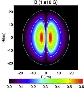
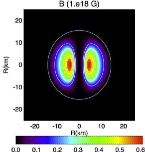
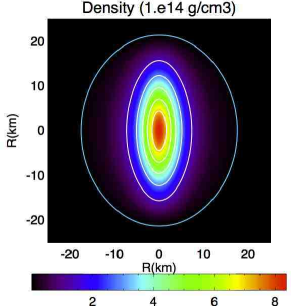
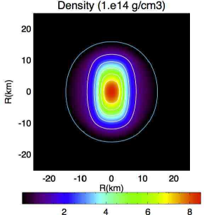
Figure 1: Meridional distribution and isocontours of the magnetic field strength $B=\sqrt{B^{\phi}B_{\phi}}$ (top) and of the baryonic density (bottom) for models with baryonic mass $M_{0}=1.68M_{\sun}$, maximum magnetic field strength $B_{\tiny{\mbox{max}}}=6.134\times 10^{17}\,\mbox{G}$, with magnetic index $m=1$ (left) and $m=2$ (right). Blue curves represent the surface of the star. Other global quantities related to these configurations are listed in Table 1.

Table 1: Global physical quantities of the equilibrium models displayed in Fig. 1 with baryonic mass $M_{0}=1.68M_{\sun}$ and maximum magnetic field strength $B_{\tiny{\mbox{max}}}=6.134\times 10^{17}\,\mbox{G}$. For the definition of the various quantities see Appendix B.

Model	$\rho_{c}$	$M$	$r_{e}$	$r_{p}/r_{e}$	$R_{\rm circ}$	$\mathscr{H}/\mathscr{W}$	$\bar{e}$	$\Phi$
	[$10^{14}\mbox{g}\,{\mbox{cm}}^{-3}$]	[$M_{\odot}$]	[km]		[km]	[$10^{-1}$]	[$10^{-1}$]	[$10^{30}\,\mbox{G}\,\mbox{cm}^{2}$]
$m=0$	8.576	1.551	12.08	1.000	14.19	0.000	0.000	0.000
$m=1$	8.430	1.596	18.10	1.139	20.15	2.013	-8.130	1.538
$m=2$	8.588	1.577	14.01	1.104	15.92	1.246	-3.730	0.862

Similar considerations hold for the distribution of the baryonic density (Fig. 1). In both cases the magnetic stresses lead to a prolate deformation of the star. This affects the internal layers even more than the outer ones. Indeed, the typical prolateness of the iso-density surfaces in the core is larger than the deformation of the stellar surface, and the external low-density layers. Interestingly, to this axial compression of the internal layers corresponds an expansion of the outer part of the star to larger radii, due to the extra pressure support provided by the magnetic field. There are two noticeable differences between the $m=1$ and $m=2$ cases, in this respect. For $m=1$ the iso-density surfaces are, to a good approximation, prolate ellipsoids, while in the $m=2$ case they tend to be more barrel-shaped. More important, despite the internal maximum magnetic field being the same, the $m=2$ case shows a much smaller deformation. This can be explained recalling that the action of the magnetic tension, responsible for the anisotropy, is $\propto B^{2}/R$ ($R$ is now the radius of curvature of the magnetic field line). For higher values of $m$ the magnetic field reaches its maximum at increasingly larger radii, resulting in a relatively smaller tension. Based on our results it is evident that a magnetic field concentrated at larger radii will produce smaller effects, than the same magnetic field, buried deeper inside. This can be rephrased in terms of currents, suggesting that currents in the outer layers have minor effects with respect to those residing in the deeper interior.

Apart from a qualitative analysis of the structure and configuration of these equilibrium models, it is possible to investigate in detail the available parameter space, and how the various quantities are related. This will allow us also to compare our results with other previously presented in literature, in particular the results by KY08 and FR12, for a purely toroidal magnetic field. KY08 and FR12 both solve for equilibrium in the correct regime for the space-time metric, described by a quasi-isotropic form. Despite this, the results are significatively different. In Fig. 2 we compare our results with KY08 and FR12 (for the case $m=1$). We plot the deviation of four quantities with respect to the unmagnetized case, as a function of the maximum value of the magnetic field strength inside the star. The deviation of a quantity $Q$ is here defined as:

$$\Delta Q=\frac{[Q(B_{\tiny{\mbox{max}}},M_{0})-Q(0,M_{0})]}{Q(0,M_{0})}.$$ (44)

The sequence refers to a set of equilibrium models, characterized by a constant baryonic mass $M_{0}=1.68M_{\sun}$, as a function of the maximum field strength $B_{\tiny{\mbox{max}}}$. Following KY08 we show: the mean deformation rate $\bar{e}$, the deviation of the gravitational mass $\Delta M$, of the circumferential radius $\Delta R_{\rm circ}$ and of the central baryonic density $\Delta\rho_{c}$. Our models are in complete agreement with FR12 and confirm the latter results against KY08. The first thing to notice is that $B_{\tiny{\mbox{max}}}$ is not a monotonic function of the magnetization constant $K_{m}$. On the contrary $B_{\tiny{\mbox{max}}}$ initially increases with $K_{m}$, till it reaches a maximum value, and then for higher values of $K_{m}$ it drops. This is due to the expansion of the star. For small values of $K_{m}$, the stellar radius is marginally affected, and an increase in $K_{m}$ leads to a higher field. However at higher values of $K_{m}$ the radius of the star is largely inflated and a further increase in $K_{m}$ translates into an expansion of the star, and a consequent reduction of the maximum internal field. If $\Delta M$, $\Delta R_{\tiny{\mbox{circ}}}$, or $\bar{e}$ are plotted against the total magnetic energy, we find that there appears to be a monotonic trend, at least in the range covered by our models. A similar effect shows up in the behaviour of the central density. For small values of $K_{m}$ the magnetic tension tends to compress the matter in the core, increasing its density. However as soon as the magnetic field becomes strong enough to cause the outer layer of the star to expand, the central density begins to drop (recall that the sequence is for a fixed baryonic mass). The same comparison with KY08 in the $m=2$ (FR12 present only the $m=1$ case) is shown in Fig. 3.

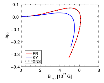
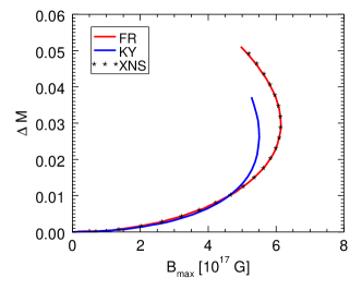
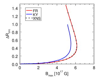
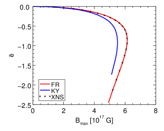
Figure 2: Variation, with respect to the unmagnetized equilibrium model, of the central baryon density $\rho_{c}$, of the gravitational mass $M$, of the circumferential radius $R_{\tiny{\mbox{circ}}}$ and of the mean deformation rate $\bar{e}$ along the equilibrium sequence of magnetized configuration with constant $M_{0}=1.68M_{\sun}$ and $m=1$. Lines represent the results by KY08 and FR12, points are our results.

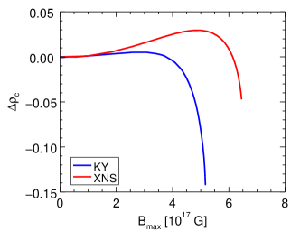
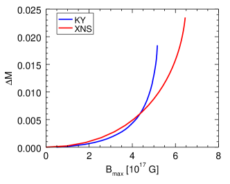
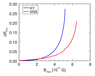
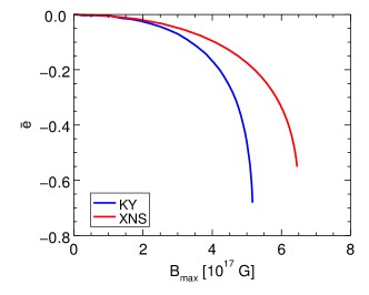
Figure 3: Same comparison as the one shown in as in Fig. 2 but for the $m=2$ case.

Following KY08 we have carried out a full sampling of the parameter space. In Fig. 4 we plot the gravitational mass $M$ as a function of the central density $\rho_{c}$ both for sequences with a constant baryonic mass $M_{0}$ and a constant magnetic flux $\Phi$. The first thing to notice is that the maximum gravitational mass, at fixed magnetic flux $\Phi$, increases with $\Phi$. Moreover for a given $\Phi$ the model with the maximum gravitational mass have also the maximum rest mass. On the other hand the minimum gravitational mass, at fixed rest mass $M_{0}$, decreases with $M_{0}$. Similarly, for a given $M_{0}$ the model with the minimal gravitational mass have also the minimum magnetic flux. The filled circles locate the maximum gravitational mass models in the sequences of constant $\Phi$. The global quantities related to these configurations are summarized in Table 2.

Interestingly, while for the vast majority of our magnetized models the gravitational mass, for a given central density, is higher than in the unmagnetized case, for small values of $\Phi$ this is not true at densities below $\sim 1.8\times 10^{15}$ g cm^-3 for $m=1$. This is a manifestation of the same effect discussed above in relation to the trend of the central density in Fig. 2. This effect was already present to a lesser extent in KY08, but not discussed.

Our set of models allows us also to construct sequences characterized by a constant magnetic field strength $B_{\tiny{\mbox{max}}}$ or a constant deformation rate $\bar{e}$. It is evident that models with a higher central density, which usually correspond to more compact stars, can harbour a higher magnetic field with a smaller deformation.

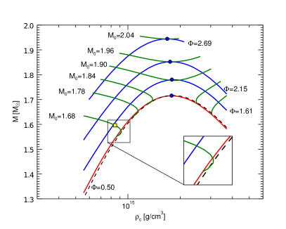
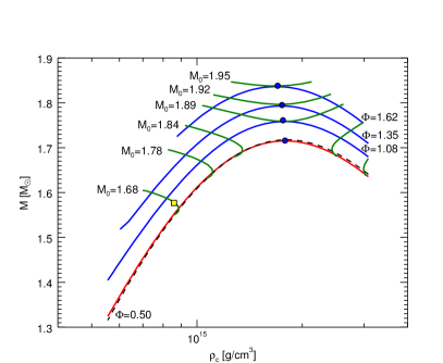
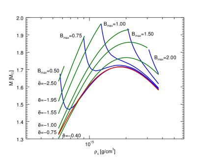
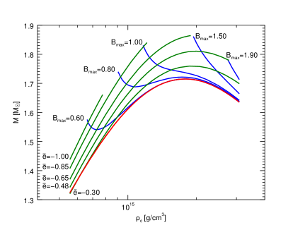
Figure 4: Sequences of equilibrium stellar models with purely toroidal field, for various fixed quantities. Top panel: with fixed baryonic mass $M_{0}$ and fixed magnetic flux $\Phi$. Bottom panel: with fixed mean deformation rate $\bar{e}$ and fixed maximum magnetic field strength $B_{\tiny{\mbox{max}}}$. Left panels show configurations with $m=1$ while right ones show configurations with $m=2$. $M_{0}$ is expressed in unit of solar masses $M_{\sun}$, $\Phi$ in unity of $10^{30}\mbox{G}\,\mbox{cm}^{2}$ and $B_{\tiny{\mbox{max}}}$ in unity of $10^{18}\mbox{G}$. The red line is the unmagnetized sequence while the black dotted lines represent equilibrium configurations with low magnetic flux $\Phi$. The filled circles locate the models with the maximum gravitational mass at fixed magnetic flux. Details of these models are listed in Table 2. The yellow squares represent the models shown in Fig. 1.

Table 2: Global quantities of the maximum mass models shown in Fig. 4. For the definition of the various quantities see Appendix B.

Model	$\rho_{c}$	$M$	$M_{0}$	$R_{\rm circ}$	$r_{p}/r_{e}$	$\mathscr{H}/\mathscr{W}$	$\bar{e}$	$B_{\tiny{\mbox{max}}}$	$\Phi$
	[$10^{14}\mbox{g}\,{\mbox{cm}}^{-3}$]	[$M_{\odot}$]	[$M_{\odot}$]	[km]		[$10^{-1}$]	[$10^{-1}$]	[$10^{18}\,\mbox{G}$]	[$10^{30}\,\mbox{G}\,\mbox{cm}^{2}$]
$m=0$	17.91	1.715	1.885	11.68	1.000	0.000	0.000	0.000	0.000
$m=1$	18.65	1.780	1.901	14.84	1.088	1.670	-4.587	1.129	1.613
	17.50	1.852	1.960	17.74	1.107	2.373	-7.833	1.216	2.150
	16.85	1.945	2.041	20.86	1.138	2.956	-11.36	1.265	2.690
$m=2$	17.69	1.761	1.890	13.22	1.067	1.330	-3.041	1.133	1.080
	17.78	1.795	1.916	13.98	1.094	1.747	-4.311	1.262	1.350
	17.00	1.838	1.950	15.07	1.115	2.158	-5.944	1.291	1.620

4.2 Purely Poloidal Field

In this section we will discuss the properties of neutron star models with a purely poloidal magnetic field. Models with a purely poloidal field have been presented in the past by BB95 . However, a direct comparison can only be done with one of their models. In fact they only present, with full details, two magnetized models with polytropic EoS. However one of them has a very high magnetic field and strong deformation, and we could not reach those conditions in our code. The polytropic index that they use is $\gamma_{a}=2$ while the polytropic constant is $K_{a}=372$, different from the fiducial value we have adopted in this study. For the model that we could reproduce, we found an agreement with the BB95 results with deviations $\lesssim 1$% for all quantities, except the magnetic dipole moment, where the error is $\sim$ a few percents. We want however to point out that our operative definition of magnetic dipole moment is different than the one given by BB95, which is valid only in the asymptotically flat limit, where magnetic field vanishes (see the discussion in Appendix B). Given that BB95 solve in the correct quasi-isotropic metric, the comparison is also a check on the accuracy of the CFC approximation. It is evident that the CFC approximation gives results that are in excellent agreement with what is found in the correct full GR regime.

In Fig. 5 we present a model with a purely poloidal field. The model has been obtained in the simple case $\xi=0$, where only linear currents are present: $J^{\phi}=\rho hk_{\rm pol}$. The model has a rest mass $M_{0}=1.680M_{\sun}$, a maximum magnetic field $B_{\tiny{\mbox{max}}}=6.256\times 10^{17}$G, and a dipole moment $\mu=2.188\times 10^{35}$ erg G^-1.

In contrast to the toroidal case, for a purely poloidal magnetic field the NS acquires an oblate shape. The magnetic field threads the entire star, and reaches its maximum at the very center. The pressure support provided by the magnetic field, leads to a flattening of the density profile in the equatorial plane. It is possible, for highly magnetized cases, to build equilibrium models where the density has its maximum, not at the center, but in a ring-like region in the equatorial plane (see Fig 6). Qualitatively, these effects are analogous to those produced by rotation. Rotation leads to oblate configurations, and for a very fast rotator, to doughnut-like density distribution. The main difference however, is that rotation acts preferentially in the outer stellar layers, leaving the central core unaffected in all but the most extreme cases. A poloidal magnetic field instead acts preferentially in the core, where it peaks.

Another difference with respect to cases with a purely toroidal field, is the fact that the magnetic field extends smoothly outside the NS surface. Surface currents are needed to confine it entirely within the star. As a consequence, from an astrophysical point of view, the dipole moment $\mu$ is a far more important parameter than the magnetic flux $\Phi$, because it is in principle an observable (it is easily measured from spin-down).

Similarly to what was done in the case of a purely toroidal magnetic field, we have built an equilibrium sequence, in the simplest case $\xi=0$, at fixed baryonic mass $M_{0}=1.680M_{\sun}$ (Fig 7). Changes in the various global quantities are shown as a function of the maximum magnetic field inside the star $B_{\rm max}$. The results in Fig 7 show that the central density $\rho_{c}$ decreases with $B_{\rm max}$ while the gravitational mass $M$, the circumferential radius $R_{\rm circ}$ and the mean deformation rate $\bar{e}$, which is now positive (oblateness), grow. As in the toroidal case, for this sequence, there appears to be a maximum value of magnetic field $B_{\rm max}\approx 6.25\times 10^{17}$ G. However, we have not been able to build models with higher magnetization, and so we cannot say if such value is reached asymptotically, or, as in the toroidal case, increasing further the magnetization, leads to a reduction of the maximum field strength. The other main qualitative difference with respect to the toroidal case is the trend of the central density, which is now a monotonic function of the maximum magnetic field. From a quantitative point of view we notice that the central density is more affected by the magnetic field. In Fig. 8 we also display the variation of the magnetic dipole moment $\mu$ along the same sequence as a function of the maximum field strength $B_{\rm max}$. The trend is linear for weak magnetic fields, and then seems to increase rapidly once the field approaches its maximum.

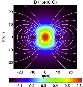
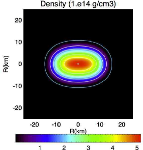
Figure 5: Left panel: magnetic field surfaces (isocontours of $\tilde{A}_{\phi}$) and distribution of the magnetic strength $B=\sqrt{B^{r}B_{r}+B^{\theta}B_{\theta}}$. Right panel: baryonic density distribution. The blue curves represent the surface of the star. The model is characterized by $M_{0}=1.68M_{\sun}$, $B_{\tiny{\mbox{max}}}=6.256\times 10^{17}\,\mbox{G}$ and magnetic dipole moment $\mu=2.188^{35}\,\mbox{erg}\,\mbox{G}^{-1}$.

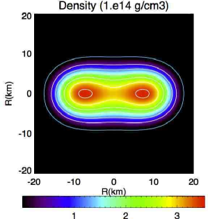
Figure 6: Baryonic density distribution for an extremely deformed configuration with a toroidal-like shape. This configuration is characterized by a baryonic rest mass $M_{0}=1.749M_{\sun}$, a gravitational mass $M=1.661M_{\sun}$, a maximum field strength $B_{\rm max}=5.815\times 10^{17}\,\mbox{G}$, a magnetic dipole moment $\mu=3.595\times 10^{35}\,\mbox{erg}\,\mbox{G}^{-1}$, a circumferential radius $R_{\rm circ}=19.33\mbox{km}$ and a mean deformation rate $\bar{e}=0.386$.

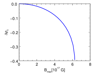
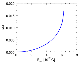
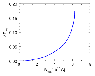
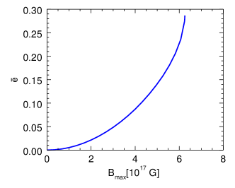
Figure 7: Variations of global quantities with respect to a non-magnetized configuration along an equilibrium sequence at fixed baryon mass $M_{0}=1.680M_{\sun}$, for models with a purely poloidal magnetic field. Notation is the same as in Fig. 2.

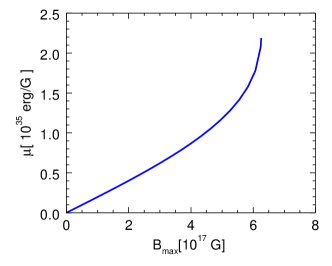
Figure 8: Magnetic dipole moment $\mu$ as a function of the maximum field strength inside the star $B_{\tiny{\mbox{max}}}$ for an equilibrium sequence with the purely poloidal magnetic field and fixed baryon mass $M_{0}=1.680M_{\sun}$.

Our choice for the magnetic function $\cal{M}$, allows us to investigate the effects of non-linear currents terms $J^{\phi}=\rho hk_{\rm pol}\xi A_{\phi}$. Unfortunately we cannot treat configurations with just non-linear currents, because in this situation the Grad-Shafanov equation has always a trivial solution $A_{\phi}=0$, and our numerical algorithm always converges to it. It is not clear if non-trivial solutions of the Grad-Shafranov equation exist in any case, and it is just the numerical algorithm that fails to find them, or if they only exist for specific values of the background quantities $(\rho,\phi,\alpha)$, and in this case it well could be that no self-consistent model can be build. So to model cases with $\xi\neq 0$, is it necessary to add a stabilizing linear current. This can be done either by adding a distributed current term $J^{\phi}=\rho hk_{\rm pol}$, or by introducing singular currents, for example surface currents. We will not consider here this latter possibility and we will investigate configurations with distributed currents alone. As anticipated, the non-linear current terms can in principle produce multipolar magnetic configurations. However, the symmetry of the magnetic field geometry is dictated by the stabilizing linear currents. Given that a current $J^{\phi}=\rho hk_{\rm pol}$, always gives dipolar dominated magnetic fields, this geometry will be preserved also by including non-linear terms. To obtain prevalent quadrupolar magnetic fields, one needs, for example, to introduce singular currents that are antisymmetric with respect to the equator. Depending on the sign of $\xi$ the non-linear current terms can be either additive or subtractive.

In Fig. 9 we show the distribution of the linear and non-linear currents inside the star, both in the additive and subtractive cases. Non-linear currents are more concentrated and they peak at larger radii. In the additive case, we succeeded in building model where non-linear currents are dominant in the outer stellar layers. On the contrary, for subtractive currents, we could not reach configurations with current inversions, and the level of the non-linear currents are at most half of the linear term.

In Fig. 10 we compare how various global quantities change, as a function of the magnetic dipole moment $\mu$ for NSs with fixed gravitational mass $M=1.551M_{\odot}$, and for various values of the parameter $\xi\in\{-10,-5,0,20,40\}$. We opted for a parametrization in terms of $\mu$ and $M$ instead of $B_{\tiny{\mbox{max}}}$ and $M_{0}$, because the former are in principle observable quantities, and as such of greater astrophysical relevance, while the latter are not.

Here we can note that, for a fixed dipole moment $\mu$, the addition of negative current terms ($\xi<0$) leads to less compact and more deformed configurations, conversely the presence of a positive current term ($\xi>0$) makes the equilibrium configurations more compact and less oblate. This might appear as contradictory: increasing currents should make deformation more pronounced. However this comparison is carried out at fixed dipole moment $\mu$. This means than any current added to the outer layers, must be compensated by a reduction of the current in the deeper ones (to keep $\mu$ constant). Giving that deformations are dominated by the core region, this explains why the star is less oblate. The opposite argument applies for subtractive currents.

Finally we have repeated a detailed parameter study, in analogy to what has been presented in the previous section, to explore the space $(\rho_{c},k_{\rm pol})$. In Fig. 11 we show various sequences characterized by either a constant baryonic mass $M_{0}$, or a constant magnetic dipole moment $\mu$, or a constant maximum field strength $B_{\tiny{\mbox{max}}}$, or a constant deformation rate $\bar{e}$. We have limited our study to models with $\xi=0$, because the addition of other currents leads in general to minor effects. Again, it is found that systems with lower central densities are in general characterized by larger deformation, for a given magnetic field and/or magnetic moment. There is, however, no inversion trend analogous to the one found for purely toroidal configurations.

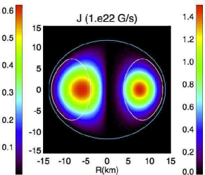
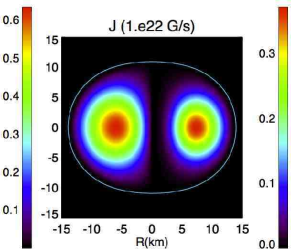
Figure 9: Comparison among models with different current distributions. Left panel: modulus of the zero-current term $J^{\phi}_{0}=\rho hk_{\rm pol}$ (left-half) and first-order one $J^{\phi}_{1}=\rho hk_{\rm pol}\xi A_{\phi}$ (right-half) for an equilibrium configuration with $\xi=20$, $M=1.551M_{\sun}$ and $\mu=1.477\times 10^{35}\,\mbox{erg}\,\mbox{G}^{-1}$. Right panel: same as the left panel but for a model with $\xi=-5$, same mass $M=1.550M_{\sun}$ and magnetic dipole moment $\mu=1.510\times 10^{35}\,\mbox{erg}\,\mbox{G}^{-1}$ . The white line locates the points where $|J^{\phi}_{1}|/|J^{\phi}_{0}|\sim 1$. The blue line represents the stellar surface.

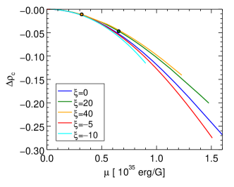
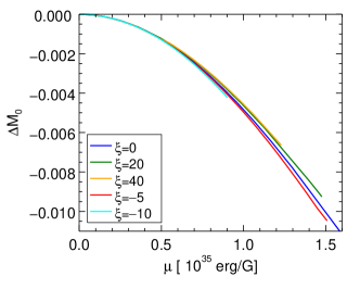
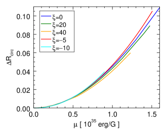
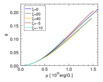
Figure 10: Variations of global quantities with respect to the non-magnetized configuration, as a function of the magnetic dipole moment, along an equilibrium sequence with fixed gravitational mass $M=1.551M_{\sun}$, and purely poloidal field. Notation is the same as in Fig. 2. Filled dots locate the points where the maximum strength of zeroth-order term $J^{\phi}_{0}=\rho hk_{\rm pol}$ is equal to the maximum strength of first-order term $J^{\phi}_{1}=\rho hk_{\rm pol}\xi A^{\phi}$. Details concerning these configurations and those which show the higher value of $\mu$ for each sequence are listed in Table 3.

Table 3: Global quantities from selected configurations belonging to the equilibrium sequences shown in Fig 10, at $M=1.551M_{\odot}$. For each value of $\xi$ we show the details for the configuration with the maximal magnetic dipole moment. For cases with $\xi=20,40$ we also present those configurations where ratio $|J_{1}|/|J_{0}|\simeq 1$. For the definition of the various quantities see Appendix B.

Model	$\rho_{c}$	$M_{0}$	$R_{\rm circ}$	$r_{p}/r_{e}$	$\bar{e}$	$\mathscr{H}/\mathscr{W}$	$B_{\tiny{\mbox{max}}}$	$\mu$	$|J_{1}|/|J_{0}|$
	[$10^{14}\mbox{g}\,{\mbox{cm}}^{-3}$]	[$M_{\sun}$]	[km]	[$10^{-1}$]	[$10^{-1}$]	[$10^{-2}$]	[$10^{17}$G]	[$10^{35}$erg G-1]
$\xi=20$	8.149	1.678	14.48	9.656	0.468	1.443	2.692	0.629	0.989
	6.810	1.665	15.54	8.420	1.773	6.656	4.595	1.477	2.421
$\xi=40$	8.426	1.680	14.35	9.827	0.127	0.979	1.417	0.118	0.990
	7.320	1.670	15.11	8.857	1.352	4.837	3.964	1.230	4.023
$\xi=-5$	6.176	1.663	15.75	7.774	2.067	7.482	6.243	1.510	0.585
$\xi=-10$	7.543	1.674	14.79	8.996	1.014	3.099	4.782	0.911	0.691

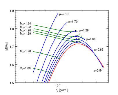
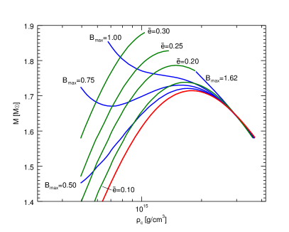
Figure 11: Left panel: equilibrium sequences with fixed magnetic field moment $\mu$ and fixed baryonic mass $M_{0}$. Right panel: equilibrium sequences with fixed deformation rate $\bar{e}$ and maximum field strength $B_{\tiny{\mbox{max}}}$. The baryonic mass is expressed in units of $M_{\sun}$, the magnetic dipole moment in units of $10^{35}\,\mbox{erg}\,\mbox{G}^{-1}$ and the maximum field strength in units of $10^{18}\mbox{G}$. The red line shows the unmagnetized sequence while the filled dots locate the configurations with maximum mass for a given dipole moment $\mu$. Parameters for these configurations are listed in Table (4).

Table 4: Global quantities from the poloidal models with maximum gravitational mass in sequences with fixed magnetic dipole moment $\mu$, shown in Fig. 11. For the definition of the various quantities see Appendix B.

$\rho_{c}$	$M$	$M_{0}$	$R_{\rm circ}$	$\mathscr{H}/\mathscr{W}$	$B_{\mbox{\tiny{max}}}$	$\bar{e}$	$r_{p}/r_{e}$	$\mu$
[$10^{14}\mbox{g}\,{\mbox{cm}}^{-3}$]	[$M_{\odot}$]	[$M_{\odot}$]	[km]	[$10^{-2}$]	[$10^{17}\,\mbox{G}$]	[$10^{-1}$]	[$10^{-1}$]	[$10^{35}\,\mbox{erg}\,\mbox{G}^{-1}$]
17.29	1.725	1.892	11.96	1.821	6.162	0.481	9.551	0.543
17.19	1.740	1.903	11.89	4.275	9.406	1.036	8.961	0.833
16.76	1.757	1.916	11.93	6.647	11.70	1.481	8.442	1.041
16.45	1.785	1.938	12.00	10.17	14.45	2.012	7.922	1.290

4.3 Mixed Field

Finally, in this subsection we will illustrate in detail the properties of TT configurations. For all the cases we present, we have adopted a functional form for $\mathcal{M}$ identical to the one used in the purely poloidal case [see Eq. (32)] but only assuming linear terms for the toroidal currents, $\xi=0$. Note, however, that the presence of a toroidal field is equivalent to the existence of an effective non-linear current term. The toroidal magnetic field is instead generated by a current term $\mathcal{I}$, given by Eq. (33). Again we have selected the simplest case: $a\neq 0$ and $\zeta=0$. We focus here on fully non-linear solutions in the strong magnetic field limit. A study of the low magnetic field limit is presented in Appendix A.

In Fig. 12 we present a typical TT model, and in particular this configuration corresponds to the one with the highest toroidal magnetic field among all our models. As anticipated, the structure of the poloidal magnetic field closely resembles what was found in the previous section, on purely poloidal models: it threads the entire star, reaches its maximum value at the center, vanishing only in ring-like region in the equatorial plane, and crosses smoothly the stellar surface. The magnetic field outside the star is dominated by its dipole component. On the other hand, the toroidal magnetic field has now a rather different structure, with respect to purely toroidal cases. It does not fill completely the interior of the star, but it is confined in a torus tangent to the stellar surface at the equator. It reaches its maximum exactly in the ring-like region where the poloidal component vanishes. Of course this behaviour is related to our choice of the poloidal current distribution, and to our requirement that they should be confined within the star. In principle it is possible to build models where the toroidal magnetic field fills the entire star, but this can only be achieved if one allows the presence of magnetospheric currents, extending beyond the stellar surface.

In the same Fig. 12 we also show the distribution of the baryonic density. As we pointed out in Sec. 4.1 a magnetic field that extends prevalently into the outer layers of the star has minor effects on the stellar properties with respect to one that penetrates also in the core region. Therefore, it is the poloidal component of the magnetic field, which is also dominant, that is mostly responsible for the deformation of the star in the TT configuration: the baryonic density distribution in fact resembles closely what we obtained in the purely poloidal configuration and the stellar shape is oblate and the external layers have a lenticular aspect.

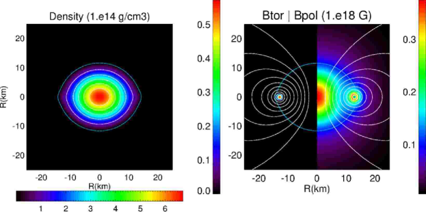
Figure 12: TT configuration with a gravitational mass $M=1.551M_{\sun}$, a baryonic mass $M_{0}=1.660$, a maximum field strength $B_{\tiny{\mbox{max}}}=5.857\times 10^{17}\,\mbox{G}$. Left panel: baryonic density distribution. Right panel: strength of the toroidal (left half) and poloidal (right half) magnetic field components, superimposed to magnetic field surfaces (isocontours of $\tilde{A}_{\phi}$. The blue curve locates the stellar surface. The other global physical quantities of this configuration are listed in the last line of Table 5.

Fig. 13 shows a comparison between the strength of the toroidal and poloidal magnetic field at the equator, for various models characterized by the same gravitational mass $M=1.551M_{\sun}$, but different values of the magnetization constants $k_{\rm pol}$ and $a$. We found that, at a fixed value of $a$, the strength of both the toroidal and poloidal field grows with $k_{\rm pol}$, while if one keeps fixed the maximum strength of the poloidal field, then the region occupied by the torus shrinks as $a$ grows.

In Fig.14 we show the relation between the magnetic dipole moment and the value of the magnetic field strength in the centre$B_{\rm c}$ along equilibrium sequences where the gravitational mass has been kept fixed, $M=1.551M_{\sun}$, for various values of $a=\{0.0,\,0.5,\,1.0,\,1.5,\,2.0\}$. It is evident that at fixed magnetic dipole moment, the field strength decreases with $a$. This can be understood if one recalls that at higher values of $a$ there is an increasing contribution to the magnetic dipole moment from currents associated to the toroidal field (the same value of $\mu$ corresponds to a lower value of $k_{\rm pol}$). As a result the value of the magnetic field at the center, which is mostly determined by the current term $\rho hk_{\rm pol}$, drops. Moreover it is also evident that there appears to be a maximum asymptotic value that the central field can reach, as we discussed in the previous section on purely poloidal configurations, and that such value is smaller for higher values of $a$.

In Fig. 15 we display, along the same sequences, how some global quantities change as a function of the magnetic dipole moment $\mu$. We stress here that this parametrization is not equivalent to the one in terms of the strength of the magnetic field at the center. We can notice that for a fixed $\mu$ the deviation from the unmagnetized case is progressively less pronounced at increasing values of $a$. This happens for the same reasons discussed above for $B_{\rm c}$. Peripheral currents, that contribute to the magnetic dipole moment, have minor effects on the magnetic field at the center. On the other hand it is the poloidal field that penetrates the core and dominates the enrgetics which is mostly responsible for these deviations. Moving to higher values of $\mu$ along the TT sequences in Fig. 15 the mean deformation rate $\bar{e}$ and the circumferential radius $R_{\rm circ}$ increase whereas the central density $\rho_{c}$ diminishes, just as in the purely poloidal configuration.

It is also interesting to look at the same quantities as parametrized in terms of the strength of the magnetic field, either the toroidal or the poloidal component. In our models, for $a<1$, the maximum magnetic field inside the star is associated with the poloidal component, and it is coincident with the central value $B_{\rm c}$, while for $a>1$ the maximum strength of the magnetic field is associated to the toroidal component. This does not seem to depend on the overall strength of the magnetic field. For the highest values the strength of the poloidal component of the magnetic field migth reach its maximum in the torus region (see the trend in Fig. 13).

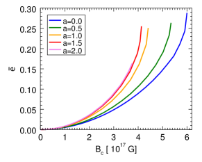
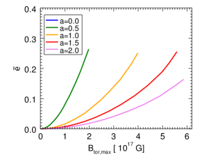
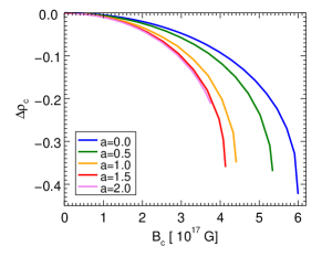
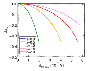
Figure 18: Mean deformation rate $\bar{e}$ (top) and $\Delta\rho_{c}$ (bottom) displayed as a function of $B_{\rm c}$ and $B_{\rm tor,max}$ along the same sequences shown in Fig. 15.

In Fig. 18 we show $\Delta\rho_{c}$ and $\bar{e}$ as a function of $B_{\rm c}$ and $B_{\rm tor,max}$. We can notice that for a fixed $B_{\rm c}$ the trend with $a$ is exactly the opposite than the one shown previously for fixed $\mu$. This might seem counter-intuitive, given that both quantities are parametrizations of the strength of the poloidal field. However, models with higher $a$, at fixed $\mu$, have weaker central fields, and smaller deviations, while models with higher $a$, at fixed $B_{\rm c}$ have higher total magnetic energy, and as such higher deviations. The effects due to the tension of the toroidal field (that would lead to a less deformed star), are dominated by the drop in the central density due to the increase of magnetic energy. For the same reason, when shown as a function of the maximum strength of the toroidal magnetic field, models show that higher values of $a$ imply smaller deviations from the unmagnetized case.

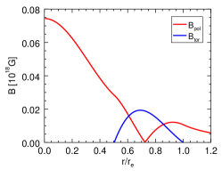
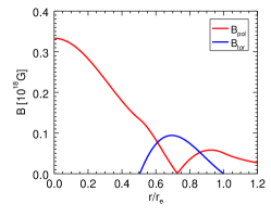
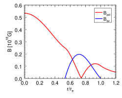
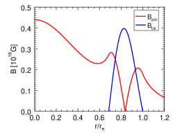
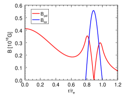
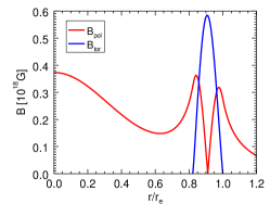
Figure 13: Profiles of the strength of the poloidal and toroidal components of the magnetic field, along the equator. $r_{e}$ is the equatorial radius. All models have the same gravitational mass $M=1.551M_{\sun}$. Top panels show three models with $a=0.5$ and $k_{\rm pol}=0.04$ (left), $k_{\rm pol}=0.18$ (center) or $k_{\rm pol}=0.31$ (right). The left bottom panel shows a model with $a=1.0$ and $k_{\rm pol}=0.23$, the central bottom panel with $a=1.5$ and $k_{\rm pol}=0.22$, and the right bottom panel with $a=2.0$ and $k_{\rm pol}=0.19$. The global physical quantities of these configuration are listed in Table 5.

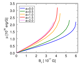
Figure 14: Magnetic dipole moment $\mu$ as a function of $B_{\rm c}$ for various values of the parameter $a$. All models have the same gravitational mass $M=1.551M_{\sun}$.

Table 5: Global quantities for various TT models with the same gravitational mass $M=1.551M_{\sun}$ but different values of both $B_{\tiny{\mbox{max}}}$ and $a$. In the last three lines we present the models with the highest maximum magnetic field that we could build, for each value of $a$. For the definition of the various quantities see Appendix B.

$a$	$\rho_{c}$	$M_{0}$	$R_{\rm circ}$	$r_{e}/r_{p}$	$\bar{e}$	$\mathscr{H}/\mathscr{W}$	$B_{\mbox{\tiny{c}}}$	$B_{\mbox{\tiny{tor,max}}}$	$\mu$	$H_{\rm m}$	$\mathscr{H}_{\mbox{\tiny{tor}}}/\mathscr{H}$
	[$10^{14}\mbox{g}\,{\mbox{cm}}^{-3}$]	[$M_{\odot}$]	[km]		[$10^{-1}$]	[$10^{-1}$]	[$10^{17}$G]	[$10^{17}$G]	[$10^{35}\,\mbox{erg}\,\mbox{G}^{-1}$]	[$10^{42}\,\mbox{G}^{2}\,\mbox{cm}^{4}$]	[$10^{-2}$]
0.5	8.488	1.680	14.24	1.000	0.033	0.011	0.745	0.194	0.173	0.031	2.893
0.5	7.890	1.675	14.70	0.935	0.715	0.251	3.338	0.944	0.862	0.791	3.228
0.5	5.373	1.650	16.88	0.723	2.636	1.285	5.344	1.974	2.308	5.512	4.082
1.0	5.545	1.647	17.41	0.733	2.510	1.455	4.409	3.983	2.790	8.079	7.262
1.5	5.454	1.645	18.11	0.711	2.552	1.566	4.134	5.582	3.199	7.752	7.282
2.0	6.713	1.660	16.40	0.816	1.636	0.880	3.758	5.857	2.152	3.234	6.696

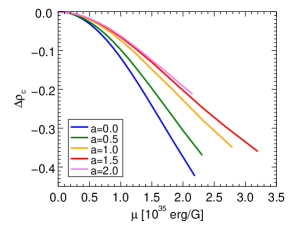
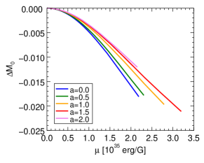
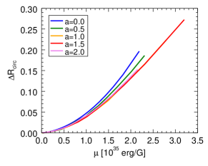
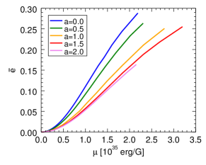
Figure 15: Behaviour of the baryonic central density $\rho_{c}$, of the baryonic mass $M_{0}$, of the circumferential radius $R_{\rm circ}$ and the mean deformation rate for TT equilibrium sequences with a fixed gravitational mass $M=1.551M_{\sun}$. All quantities are shown as a function of the magnetic dipole moment $\mu$. The models corresponding to the extreme cases for each sequence are presented in details in the last four lines in Table 5.

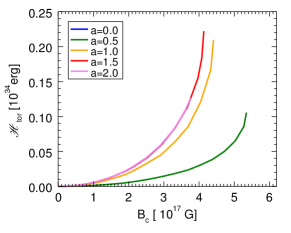
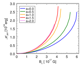
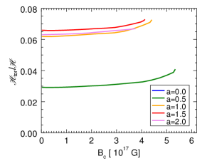
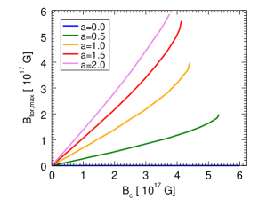
Figure 16: Top left panel: toroidal magnetic energy $\mathscr{H}_{\rm tor}$. Top right panel: poloidal magnetic energy $\mathscr{H}_{\rm pol}$. Bottom left panel: ratio of the toroidal magnetic energy $\mathscr{H}_{\rm tor}$ to the total magnetic energy $\mathscr{H}$. Right bottom panel: maximum value of the toroidal magnetic field strength $B_{\rm tor,max}$. All quantities are plotted as a function of the central magnetic field strength $B_{\rm c}$ along the same sequences shown in Fig. 15.

In Fig. 16 these same sequences are shown in terms of their energy content. We note that, at fixed $B_{\rm c}$, the equilibrium configurations with higher $a$ are characterized by a higher value of both the total toroidal magnetic field energy $\mathscr{H}_{\rm tor}$, and the poloidal magnetic field energy $\mathscr{H}_{\rm tor}$, as expected. It is also evident that the parameter $a$ regulates the ratio of energy in the toroidal and poloidal components of the magnetic field, $\mathscr{H}_{\rm tor}/\mathscr{H}$. We see that the ratio $\mathscr{H}_{\rm tor}/\mathscr{H}$ tends to a constant in the limit of a negligible magnetic field. In the last panel in Fig. 16 we also show the relation between $B_{\rm c}$ and the maximum strength of the toroidal magnetic field $B_{\rm tor,max}$. The ratio $\mathscr{H}_{\rm tor}/\mathscr{H}$ shows a clear maximum at $\sim 0.07$ for $a\simeq 1.5$. For smaller values of $a$ this ratio increases because the strength of the toroidal field increases, however, for $a\gtrsim 1$, the volume taken by the torus, where the toroidal field is confined, begins to drop substantially, and this leads to a smaller total energy of the toroidal component. The net effect of the torus shrinkage over $\mathscr{H}_{\rm tor}/\mathscr{H}$ is also evident from Fig. 17 where the magnetic energy ratio is shown as a function of the parameter $a$ along a sequence with fixed $B_{\rm c}=2\times 10^{17}$ G.

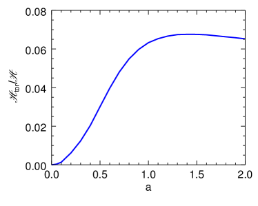
Figure 17: Ratio of the toroidal magnetic energy $\mathscr{H}_{\rm tor}$ to the total magnetic energy $\mathscr{H}$ as a function of the parameter $a$ along a sequence with fixed gravitational mass $M=1.551M_{\odot}$ and central magnetic field strength $B_{\rm c}=2\times 10^{17}$ G.

Finally in Fig 19 we show the magnetic helicity $H_{m}$ as a function of either the field strength at the centre$B_{\rm c}$ or the maximum strength of the toroidal magnetic field $B_{\rm tor,max}$. The magnetic helicity is an important quantity in MHD because it is conserved in the limit of infinite conductivity, and it can be shown that it is dissipated on a much longer timescale than the magnetic energy in the resistive case (Candelaresi & Brandenburg, 2011). It is generally expected that MHD will rapidly relax to configurations that minimize magnetic energy, keeping fixed the magnetic helicity. At a fixed $B_{\rm c}$, $H_{m}$ increases up to $a\simeq 1.5$, then drops, for the same reason discussed above for the energetics. Instead, at a fixed $B_{\rm tor,max}$, $H_{m}$ decreases with $a$ since, in this case, the same toroidal magnetic strength, corresponds to a weaker poloidal field.

In general we found a qualitative agreement with previous results (Lander & Jones, 2009; Ciolfi et al., 2009; Ciolfi, Ferrari & Gualtieri, 2010; Ciolfi & Rezzolla, 2013), concerning the shape, deformation, and expected distribution of the poloidal and toroidal components of the magnetic field. In all of our models, the poloidal component is dominant and the ratio $\mathscr{H}_{\rm tor}/\mathscr{H}<0.07$. This agrees with previous results where it was shown that only poloidally dominated models could be built for simple electric current distributions, although recently a more complicated prescription for the currents allowed to build toroidally dominated models (Ciolfi & Rezzolla, 2013). For strong fields, inducing an appreciable deformation, a direct comparison is possible only with previous results by Lander & Jones (2009). They adopt a different value of $\zeta=0.1$ instead of $0$, their values of $a$ are not directly comparable with ours due to the different choice of units, and their reference unmagnetized model is different. Notwithstanding these differences, our results agree with theirs, on many aspects. A direct quantitative, comparison with results by Ciolfi et al. (2009); Ciolfi, Ferrari & Gualtieri (2010); Ciolfi & Rezzolla (2013) is also not straightforward, because their choice for the functional form of the current associated with the toroidal field, Eq. 33, is different from our (they assume that the current is a cubic function of the vector potential while we assume it to be linear). Their perturbative approach in principle corresponds to a low magnetic field limit. A more detailed discussion in this limit is presented in Appendix A.

In the fully non linear regime, given that we do not impose any constrain on the shape of the stellar surface, and allow for oblate configurations, our field may adjust to this change in shape. Indeed, as shown in Fig. 15 we found that, for strong fields, inducing an appreciable deformation, the ratio $\mathscr{H}_{\rm tor}/\mathscr{H}$ is higher that for the weak field limit by about $10-15\%$.

We want to stress here that the Grad-Shafranov equation Eq. (31), in cases where the currents are non linear in the vector potential $A_{\phi}$, becomes a non linear Poisson-like equation, that in principle might admit multiple solutions (local uniqueness is not guaranteed). This is a known problem (Ilgisonis & Pozdnyakov, 2003), so that we cannot safely say that these are the only possible equilibria.

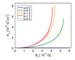
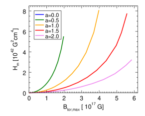
Figure 19: Magnetic helicity $H_{m}$ as a function of the central magnetic field strength $B{\rm c}$ (left) and as a function of the maximum toroidal magnetic field strength $B_{\rm tor,max}$ (left) along the same equilibrium sequences shown in Fig. 15.

5 Conclusions

Magnetic fields are a key element in the physics and phenomenology of NSs. Virtually nothing of their observed properties can be understood without considering their effects. In particular, the geometry of the magnetic field plays an important role, and even small differences can lead to changes in the physical processes that might be important for NS phenomenology (Harding & Muslimov, 2011). Here we have investigated the role that a very strong magnetic field has in altering the structure, by inducing deformations. For the first time we have derived equilibrium configurations, containing magnetic field of different geometries, assuming the metric to be Conformally Flat. This is a further improvement on previous works, which where either done in a Newtonian or perturbative regime, and allow us to handle very strong fields, and to take into account the typical non-linearity of Einstein equations.

We have presented a general formalism to model magnetic field of different geometry, and illustrated our numerical technique. The comparison with previous results (when available) has shown that the assumption of a conformally flat metric leads to results that are indistinguishable, within the accuracy of the numerical scheme, from those obtained in the correct regime. The simplifications in our approach do not compromise the accuracy of the results, while greatly simplifying their computation.

For the first time we have carried out a detailed parameter study, where the role of current distributions was analyzed, for various geometries of the magnetic field. We briefly summarize here the key results:

• the characteristic deformation induced by a purely toroidal field, fully confined below the stellar surface, is prolate: the magnetic field acts by compressing the internal layers of the star around its symmetry axis, causing, on the other hand, an expansion of the outer layers;

• given the same strength, magnetic fields concentrated in the outer part of the star, lead to smaller deformations, with respect to magnetic fields concentrated in the internal regions;

• a purely poloidal field, that in our case extends also outside the star, leads to oblate equilibrium configurations: the magnetic stresses act preferentially in the central regions, where the field peaks, leading to a flatter density profile perpendicularly to the axis itself. We can also obtain doughnut-like configurations where the density maximum is not at the center;

• the presence of additional currents located in the outer layers of the stars, leads only to marginal changes in its structure, and on the shape of the magnetic field lines outside the stellar surface;

• for the same maximum magnetic field inside the star, purely poloidal configuration, can be characterized by smaller deformations, than purely toroidal ones (about a factor one half in the $m=1$ case). However for higher values of $m$ this trend might be reversed;

• we have computed Twisted-Torus configurations in the non-perturbative regime. We confirm previous results, in either the Newtonian or the perturbative regime, that only models where the poloidal component is energetically dominant can be built for simple electric current distributions [this limitation could be avoided using more complex prescriptions for the currents as shown by Ciolfi & Rezzolla (2013)]. These show oblate deformations that are almost completely due to the poloidal field, acting on the interior;

• for a fixed central density, a higher magnetic field gives a higher eccentricity, a higher radius and a higher gravitational mass;

• the more compact configurations, having a higher central density, can support stronger magnetic fields, and show much smaller deformations.

Our results are clearly indicative, that the magnetic energy, or the maximum strength of the magnetic field, are in general not good indicators of the possible deformation of the NS. The current distribution is a key parameter: magnetic field concentrated in the outer layers of the stars are less important than similar fields located in the deeper interior. Given that the magnetic field geometry, might strongly depend on the details of the NS formation (the stratification of differential rotation, the location of the convective region, etc…), one should be careful to make general statements based only on energetic arguments.

We plan to further extend this work, by investigating also rotating configurations and/or NS models with magnetospheric currents, that we have not touched upon here, and trying to provide some more quantitative estimates on the possible GW emission from this objects and its dependence on the strength and structure of the magnetic field.

The updated XNS code for building magnetized neutron star equilibria is publicly available for the community at www.arcetri.astro.it/science/ahead/XNS/.

Appendix A Limit of Weak Magnetic Fields

In the limit of a weak magnetic field (i.e. for $\mathscr{H}\ll M$), one can safely assume that the metric terms $\alpha$ and $\psi$ are the same as in the unmagnetized case (up to corrections of the order of $\mathscr{H}/M$). For our models, which are also static, these are only function of the radial coordinate $r$. In this limit, for our choice of magnetic current distributions, $\xi=0$ and $\zeta=0$, both the currents associated to the toroidal field and the magnetic field itself become linear functions of the vector potential $A_{\phi}$. For a given value of the twisted torus magnetization constant $a$, the Grad-Shafranov equation, Eq. (31), contains only terms linear in $A_{\phi}$ ($A_{\phi}$ is now a linear function of the poloidal magnetization constant $k_{\rm pol}$). This implies that in the weak magnetic field limit, the magnetic field structure and the geometry of the magnetic field lines are independent of the strength of the magnetic field. It is thus meaningful to talk about a low magnetization limit, without reference to the exact value of the magnetic field. This is quite different from previous results, published in literature. For example the works by Ciolfi et al. (2009) and by Glampedakis, Andersson & Lander (2012), following the choice initially suggested by Tomimura & Eriguchi (2005), all assume that the function $\mathcal{I}$ is quadratic in $A_{\phi}$ [qualitative analogous to taking $\zeta=1$ in our formalism, even if their functional form for $\mathcal{I}$ is different from our generic form Eq. (33)]. This implies that the currents associated to the toroidal field are cubic in $A_{\phi}$, and the Grad-Shafranov equation now contains terms that are nonlinear in $A_{\phi}$. The same holds for the choice presented by Lander & Jones (2009) which is equivalent to take $\zeta=0.1$. In these cases the magnetic field structure is also a function of the magnetic field strength, and one cannot talk of a generic low field limit, but the exact value of the field strength must be specified.

Let us briefly describe here the properties of our solution in the limit of a small field. We will consider a fiducial model, with a central density $\rho_{\rm c}=8.515\times 10^{14}$ g cm^-3, corresponding to a gravitational mass $M=1.551M_{\odot}$, and a radius $R_{\rm circ}=14.24$ km. For convenience, all our results are shown in the case of a magnetic field with a typical strength $\approx 10^{12}$G (they can however be rescaled to higher/lower values because of the linearity implied by our choice for the distribution of the currents).

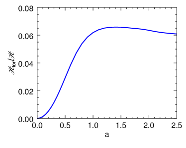
Figure 20: Ratio of the toroidal magnetic energy $\mathscr{H}_{\rm tor}$ to the total magnetic energy $\mathscr{H}$ in the weak field limit, as function of the parameter $a$, for our fiducial NS model with $M=1.551M_{\odot}$.

In Fig.20, the ratio of magnetic energy carried by the toroidal component of the field, over the total magnetic energy is shown as a function of the twisted torus magnetization constant $a$. It is evident that it is not possible to reach configurations that are toroidally dominated. In Fig.21, we show the equatorial profile of the poloidal and toroidal components of the magnetic field, for various values of the parameter $a$, as was done in Fig.13 for the case of a much stronger magnetic field. It is interesting to notice that, as was found in previous studies, the region occupied by the toroidal field tends to shrink toward the surface of the star (about 70% from $a=0.1$ to $a=2.5$). The effect is the same as seen in previous works, that used a different current’s distribution. In the same plot, done keeping the poloidal magnetization constant $k_{\rm pol}$ fixed, it is also possible to see the contribution of the current associated to the toroidal field, to the net dipole moment (the value of the polar field increases with $a$). Again, as was found in the case of a strong field, these peripheral current contribute only marginally (about 20% for $a=2.5$) to the net dipole moment.

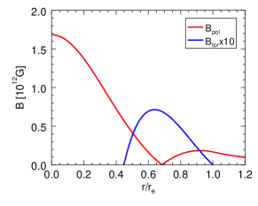
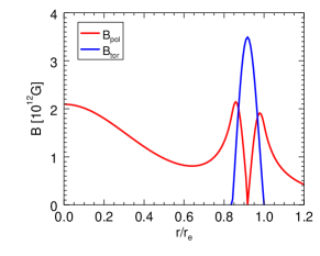
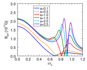
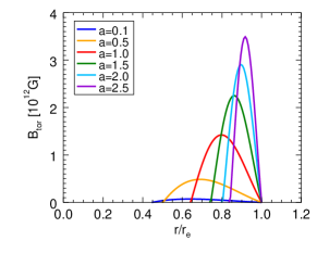
Figure 21: Upper panels: profiles of the strength of the poloidal and toroidal components of the magnetic field, along the equator, in the weak field limit, for our fiducial NS model with $M=1.551M_{\odot}$ and $k_{\rm pol}=10^{-6}$. $r_{e}$ is the equatorial radius. Upper left panel is a model with $a=0.1$. Upper right panel is a case with $a=2.5$. Lower panels: the strength of the poloidal (left) and toroidal (right) magnetic field at the equator for various values of the parameter $a$. The shrinkage of the torus region, as well as the contribution to the poloidal field by extra currents associated to the toroidal field is evident.

Finally, in this low magnetic field limits, it is possible to investigate the multipolar content of the magnetic field, and how does it change with respect to the parameter $a$ (i.e. to the ratio of toroidal magnetic field energy over total magnetic energy). A simple way to compare the various multipole terms is to look at the relative strength of the $C_{l}$ terms in the expansion of the vector potential Eq. (43), with $C_{1}$ indicating the dipole term. This is not possible for stronger fields, because the metric terms are no longer just a function of $r$, and the $C_{l}$ will also contain a geometrical contribution from the metric, which we cannot separate (spherical harmonics are not eigenfunctions of the angular part of the Laplacian in a generically curved spacetime). In Fig. 22 we show the values of various $C_{l}$ terms (normalized to the dipole one) as a function of radius. As expected, our magnetic configurations are always dominated by the dipole term. The various multipoles reach a maximum at the location of the torus, and then drop outside of the star as $r^{-(l+1)}$. In the case $a=0.1$ the various multipoles are more than 3-4 orders of magnitude smaller than the dipole term, and in general each multipole of order $l$ is about one order of magnitude smaller than the preceding one of order $l-1$ (for smaller values of $a$ the various multipoles are so small that they are essentially compatible with being due to numerical noise). In the case $a=2.5$ the multipolar content of the magnetic field is much higher: the quadrupole term $l=3$ is only a factor 10 (at peak) smaller than the dipole term, and in general the ratio between two successive multipoles is only of the order of a few.

It this low magnetic field limit, when the metric terms are essentially independent of the magnetic field strength, we have verified that in order to get converged solutions of the Grad-Shafranov equation, Eq. (31), we need to truncate our decomposition of the vector potential into spherical harmonics, Eq. (43), at a $l_{\rm max}$ such that all the neglected multipoles have at least an amplitude $C_{l>l_{\rm max}}/C_{1}<10^{-5}$. Please note that, while the overall accuracy of our models is $\sim 10^{-3}$, the accuracy of the elliptic solver of the Grad-Shafranov equation, is $\sim 10^{-7}$. In fact multipoles with amplitude less than $10^{-7}$ times the leading dipole term, are dominated by numerical noise (see for example the behaviour of the $C_{l=9}$ terms in the left panel of Fig. 22).

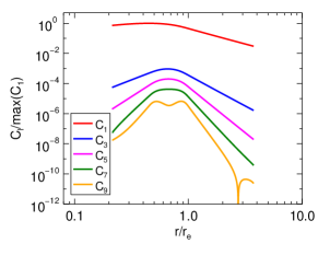
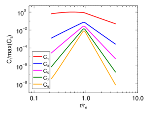
Figure 22: Radial profiles of the norm of the $C_{l}(r)$ terms in the harmonic decomposition of the vector potential [see Eq. 43], in the weak field limit. The values are normalized to the maximum of the $C_{1}(r)$, for convenience. Left panel: $a=0.1$. Right panel: $a=2.5$.

Appendix B Global Physical Quantities

To characterise the equilibrium models obtained with our numerical scheme we have computed a wide set of global physical quantities that allow us to provide a parametrization, as complete as possible. Here we give their definition for the case of static magnetized configurations, described within the CFC approximation.

The most relevant are: the gravitational mass

$$M:=\int\left(e+3p+B^{2}\right)\alpha\psi^{6}\sin\theta\,drd\theta d\phi,$$ (45)

the baryonic mass

$$M_{0}:=\int\rho\psi^{6}r^{2}\sin\theta\,drd\theta d\phi,$$ (46)

the proper mass

$$M_{p}:=\int e\psi^{6}r^{2}\sin\theta\,drd\theta d\phi,$$ (47)

the total magnetic energy

$$\mathscr{H}:=\frac{1}{2}\int B^{2}\psi^{6}r^{2}\sin\theta\,drd\theta d\phi,$$ (48)

the magnetic energy in the toroidal component

$$\mathscr{H}_{\rm tor}:=\frac{1}{2}\int B^{\phi}B_{\phi}\psi^{6}r^{2}\sin\theta\,drd\theta d\phi,$$ (49)

the magnetic energy in the poloidal component

$$\mathscr{H}_{\rm pol}:=\frac{1}{2}\int(B^{r}B_{r}+B^{\theta}B_{\theta})\psi^{6}r^{2}\sin\theta\,drd\theta d\phi,$$ (50)

and the binding energy

$$\mathscr{W}:=M-M_{p}-\mathscr{H},$$ (51)

where the integrals are defined over the all three-dimensional space.

In order to characterise the geometrical properties of the magnetic field, other quantities must be introduced. When the magnetic configuration possesses a toroidal component we can evaluate the flux of the toroidal magnetic field through a meridional half-plane which, analogously to KY08, is given by

$$\Phi:=\int_{0}^{\pi}d\theta\int_{0}^{\infty}\sqrt{B^{\phi}B_{\phi}}\psi^{4}r\,dr.$$ (52)

In the presence of a poloidal magnetic field we can estimate the magnetic dipole moment $\mu$ of the star. This is usually defined (see BB95) by the leading term of the asymptotic behaviour of the magnetic field components at $r\rightarrow\infty$, where the space-time metric is flat. However this definition, in our opinion, is not well suited for a numerical scheme. At $r\rightarrow\infty$ the magnetic field vanishes, and it is not numerically safe, due to interpolation and round-off errors, to compute a finite quantity as the ratio of two vanishing ones. On the other hand, if computed at a finite distance, this definition might introduce errors due to the metric curvature. Since our numerical scheme does not use a compactified domain, and extends only over a few stellar radii outside a NS, we have derived a definition of magnetic dipole moment that takes into account the curvature of space-time. This allows us to measure the dipole moment at finite radii, and we have verified that the value does not depend on the radius, as expected. From a multipole expansion of Eq. (31), assuming that outside the star the line element is well approximated by the Schwarzschild solution and selecting the dipole term ($l=1$), one can find a simple relation that connects the dipole moment $\mu$ to the $\phi-$component of the vector potential $\tilde{A}_{\phi}$, the gravitational mass $M$ and the radial coordinate $r$, namely

$$\tilde{A}_{\phi}=\mu\left(1+\frac{M}{4r}\right)\frac{\sin\theta}{r^{2}}.$$ (53)

In the case of mixed field configurations another important global topological quantity is the magnetic helicity. Following Ciolfi et al. (2009) the total magnetic helicity $H_{\rm m}$ can be defined as

$$H_{\rm m}:=\int H^{0}_{\rm m}\alpha\psi^{6}r^{2}\sin\theta\,drd\theta d\phi,$$ (54)

where $H^{0}_{\rm m}$ is the time component of the helicity four-current

$$H_{\rm m}^{\alpha}:=-\frac{1}{2}\epsilon^{\alpha\beta\mu\nu}A_{\beta}F_{\mu\nu}.$$ (55)

In our case the definition reduces simply to

$$H_{\rm m}=\int(B^{i}A_{i})\psi^{6}r^{2}\sin\theta\,drd\theta d\phi,$$ (56)

where, using the gauge freedom of the vector potential, we can impose $A_{r}=0$ and express $A_{\theta}$ in function of $A_{\phi}$ as

$$A_{\theta}=\frac{-1}{\sin\theta}\int_{\infty}^{r}\frac{\psi^{2}}{\alpha}\mathcal{I}(A_{\phi})dr^{\prime}.$$ (57)

Finally there are global quantities related exclusively to the shape and deformation of the star. These are the equatorial radius $r_{e}$, the polar radius $r_{p}$, the circumferential radius

$$R_{\rm circ}:=\psi^{2}(r_{e},\pi/2)r_{e}.$$ (58)

and the mean deformation that, following KY08, is defined by

$$\bar{e}:=\frac{I_{zz}-I_{xx}}{I_{zz}},$$ (59)

where $I_{zz}$ and $I_{xx}$ are the moment of inertia respectively in the parallel and orthogonal direction to the axis of symmetry

$$I_{zz}:=\int er^{4}\sin^{3}\theta drd\theta d\phi$$ (60)

$$I_{xx}:=\frac{1}{2}\int er^{4}\sin\theta(1+\cos^{2}\theta)drd\theta d\phi.$$ (61)

As was just pointed out in FR12 this definition of $\bar{e}$ is strictly Newtonian and may be not suitable for estimating the gravitational-wave emission of a rotating distorted star.

References

- Alcubierre (2008) Alcubierre M., 2008, Introduction to 3+1 Numerical Relativity. Oxford University Press
- Arnowitt, Deser & Misner (1959) Arnowitt R., Deser S., Misner C. W., 1959, Physical Review, 116, 1322
- Baade & Zwicky (1934) Baade W., Zwicky F., 1934, Physical Review, 46, 76
- Bocquet et al. (1995) Bocquet M., Bonazzola S., Gourgoulhon E., Novak J., 1995, A&A, 301, 757
- Bonanno, Rezzolla & Urpin (2003) Bonanno A., Rezzolla L., Urpin V., 2003, A&A, 410, L33
- Braithwaite (2009) Braithwaite J., 2009, MNRAS, 397, 763
- Braithwaite & Nordlund (2006) Braithwaite J., Nordlund Å., 2006, A&A, 450, 1077
- Braithwaite & Spruit (2006) Braithwaite J., Spruit H. C., 2006, A&A, 450, 1097
- Bucciantini & Del Zanna (2011) Bucciantini N., Del Zanna L., 2011, A&A, 528, A101
- Bucciantini & Del Zanna (2013) —, 2013, MNRAS, 428, 71
- Bucciantini et al. (2012) Bucciantini N., Metzger B. D., Thompson T. A., Quataert E., 2012, MNRAS, 419, 1537
- Bucciantini et al. (2009) Bucciantini N., Quataert E., Metzger B. D., Thompson T. A., Arons J., Del Zanna L., 2009, MNRAS, 396, 2038
- Burrows et al. (2007) Burrows A., Dessart L., Livne E., Ott C. D., Murphy J., 2007, ApJ, 664, 416
- Candelaresi & Brandenburg (2011) Candelaresi S., Brandenburg A., 2011, Phys. Rev. E, 84, 016406
- Carter (1970) Carter B., 1970, Communications in Mathematical Physics, 17, 233
- Carter (1973) —, 1973, in Black Holes (Les Astres Occlus), Dewitt C., Dewitt B. S., eds., pp. 57–214
- Chandrasekhar & Fermi (1953) Chandrasekhar S., Fermi E., 1953, ApJ, 118, 116
- Ciolfi, Ferrari & Gualtieri (2010) Ciolfi R., Ferrari V., Gualtieri L., 2010, MNRAS, 406, 2540
- Ciolfi et al. (2009) Ciolfi R., Ferrari V., Gualtieri L., Pons J. A., 2009, MNRAS, 397, 913
- Ciolfi & Rezzolla (2013) Ciolfi R., Rezzolla L., 2013, MNRAS
- Cordero-Carrión et al. (2009) Cordero-Carrión I., Cerdá-Durán P., Dimmelmeier H., Jaramillo J. L., Novak J., Gourgoulhon E., 2009, Phys. Rev. D, 79, 024017
- Cutler (2002) Cutler C., 2002, Phys. Rev. D, 66, 084025
- Dall’Osso & Stella (2007) Dall’Osso S., Stella L., 2007, Ap&SS, 308, 119
- Del Zanna & Chiuderi (1996) Del Zanna L., Chiuderi C., 1996, A&A, 310, 341
- Del Zanna et al. (2007) Del Zanna L., Zanotti O., Bucciantini N., Londrillo P., 2007, A&A, 473, 11
- Feroci et al. (2012) Feroci M. et al., 2012, Experimental Astronomy, 34, 415
- Ferraro (1954) Ferraro V. C. A., 1954, ApJ, 119, 407
- Frieben & Rezzolla (2012) Frieben J., Rezzolla L., 2012, MNRAS, 427, 3406
- Fujisawa, Yoshida & Eriguchi (2012) Fujisawa K., Yoshida S., Eriguchi Y., 2012, MNRAS, 422, 434
- Glampedakis, Andersson & Lander (2012) Glampedakis K., Andersson N., Lander S. K., 2012, MNRAS, 420, 1263
- Gourgoulhon (2010) Gourgoulhon E., 2010, ArXiv e-prints
- Gourgoulhon (2012) Gourgoulhon E., ed., 2012, Lecture Notes in Physics, Berlin Springer Verlag, Vol. 846, 3+1 Formalism in General Relativity
- Gourgoulhon et al. (2011) Gourgoulhon E., Markakis C., Uryū K., Eriguchi Y., 2011, Phys. Rev. D, 83, 104007
- Gualtieri, Ciolfi & Ferrari (2011) Gualtieri L., Ciolfi R., Ferrari V., 2011, Classical and Quantum Gravity, 28, 114014
- Harding & Muslimov (2011) Harding A. K., Muslimov A. G., 2011, ApJLett, 726, L10
- Haskell et al. (2008) Haskell B., Samuelsson L., Glampedakis K., Andersson N., 2008, MNRAS, 385, 531
- Hewish et al. (1968) Hewish A., Bell S. J., Pilkington J. D. H., Scott P. F., Collins R. A., 1968, Nature, 217, 709
- Ilgisonis & Pozdnyakov (2003) Ilgisonis V., Pozdnyakov Y., 2003, in APS Meeting Abstracts, p. 1107P
- Kiuchi, Kotake & Yoshida (2009) Kiuchi K., Kotake K., Yoshida S., 2009, ApJ, 698, 541
- Kiuchi & Yoshida (2008) Kiuchi K., Yoshida S., 2008, Phys. Rev. D, 78, 044045
- Konno (2001) Konno K., 2001, A&A, 372, 594
- Lander & Jones (2009) Lander S. K., Jones D. I., 2009, MNRAS, 395, 2162
- Lander & Jones (2012) —, 2012, MNRAS, 424, 482
- MacFadyen & Woosley (1999) MacFadyen A. I., Woosley S. E., 1999, ApJ, 524, 262
- Markey & Tayler (1973) Markey P., Tayler R. J., 1973, MNRAS, 163, 77
- Markey & Tayler (1974) —, 1974, MNRAS, 168, 505
- Mastrano, Lasky & Melatos (2013) Mastrano A., Lasky P. D., Melatos A., 2013, MNRAS, 434, 1658
- Mastrano et al. (2011) Mastrano A., Melatos A., Reisenegger A., Akgün T., 2011, MNRAS, 417, 2288
- Mereghetti (2008) Mereghetti S., 2008, A&A Rev., 15, 225
- Metzger et al. (2011) Metzger B. D., Giannios D., Thompson T. A., Bucciantini N., Quataert E., 2011, MNRAS, 413, 2031
- Miketinac (1975) Miketinac M. J., 1975, Ap&SS, 35, 349
- Monaghan (1965) Monaghan J. J., 1965, MNRAS, 131, 105
- Monaghan (1966) —, 1966, MNRAS, 134, 275
- Norris & Bonnell (2006) Norris J. P., Bonnell J. T., 2006, ApJ, 643, 266
- Oron (2002) Oron A., 2002, Phys. Rev. D, 66, 023006
- Ostriker & Hartwick (1968) Ostriker J. P., Hartwick F. D. A., 1968, ApJ, 153, 797
- Pons et al. (1999) Pons J. A., Reddy S., Prakash M., Lattimer J. M., Miralles J. A., 1999, ApJ, 513, 780
- Prendergast (1956) Prendergast K. H., 1956, ApJ, 123, 498
- Rheinhardt & Geppert (2005) Rheinhardt M., Geppert U., 2005, A&A, 435, 201
- Roberts (1955) Roberts P. H., 1955, ApJ, 122, 508
- Romani et al. (2012) Romani R. W., Filippenko A. V., Silverman J. M., Cenko S. B., Greiner J., Rau A., Elliott J., Pletsch H. J., 2012, ApJLett, 760, L36
- Rowlinson et al. (2010) Rowlinson A. et al., 2010, MNRAS, 409, 531
- Roxburgh (1966) Roxburgh I. W., 1966, MNRAS, 132, 347
- Spruit (2009) Spruit H. C., 2009, in IAU Symposium, Vol. 259, IAU Symposium, Strassmeier K. G., Kosovichev A. G., Beckman J. E., eds., pp. 61–74
- Tayler (1973) Tayler R. J., 1973, MNRAS, 161, 365
- Thompson & Duncan (1996) Thompson C., Duncan R. C., 1996, ApJ, 473, 322
- Tomimura & Eriguchi (2005) Tomimura Y., Eriguchi Y., 2005, MNRAS, 359, 1117
- Viganò et al. (2013) Viganò D., Rea N., Pons J. A., Perna R., Aguilera D. N., Miralles J. A., 2013, MNRAS, 434, 123
- Wilson & Mathews (2003) Wilson J. R., Mathews G. J., 2003, Relativistic Numerical Hydrodynamics
- Wilson, Mathews & Marronetti (1996) Wilson J. R., Mathews G. J., Marronetti P., 1996, Phys. Rev. D, 54, 1317
- Woltjer (1960) Woltjer L., 1960, ApJ, 131, 227
- Woosley (1993) Woosley S. E., 1993, ApJ, 405, 273
- Wright (1973) Wright G. A. E., 1973, MNRAS, 162, 339
- Yazadjiev (2012) Yazadjiev S. S., 2012, Phys. Rev. D, 85, 044030
- Yoshida, Yoshida & Eriguchi (2006) Yoshida S., Yoshida S., Eriguchi Y., 2006, ApJ, 651, 462