Scaling of maximum probability density functions of velocity and temperature increments in turbulent systems

Abstract

In this paper, we introduce a new way to estimate the scaling parameter of a self-similar process by considering the maximum probability density function (pdf) of tis increments. We prove this for $H$-self-similar processes in general and experimentally investigate it for turbulent velocity and temperature increments. We consider turbulent velocity database from an experimental homogeneous and nearly isotropic turbulent channel flow, and temperature data set obtained near the sidewall of a Rayleigh-Bénard convection cell, where the turbulent flow is driven by buoyancy. For the former database, it is found that the maximum value of increment pdf $p_{\max}(\tau)$ is in a good agreement with lognormal distribution. We also obtain a scaling exponent $\alpha\simeq 0.37$, which is consistent with the scaling exponent for the first-order structure function reported in other studies. For the latter one, we obtain a scaling exponent $\alpha_{\theta}\simeq 0.33$. This index value is consistent with the Kolmogorov-Obukhov-Corrsin scaling for passive scalar turbulence, but different from the scaling exponent of the first-order structure function that is found to be $\zeta_{\theta}(1)\simeq 0.19$, which is in favor of Bolgiano-Obukhov scaling. A possible explanation for these results is also given.

I Introduction

Since Kolmogorov’s 1941 (K41) milestone work, the invariant properties of small-scale structures have been widely investigated during the last four decades.Kolmogorov (1941); Anselmet et al. (1984); Frisch (1995); Sreenivasan and Antonia (1997); Lohse and Xia (2010) The invariant properties are characterized by a series of scaling exponents $\zeta(q)$, which is traditionally extracted by the classical structure function (SF) analysis $S_{q}(\ell)=\langle\Delta u_{\ell}(r)^{q}\rangle\sim\ell^{\zeta(q)}$ that has been documented very well for turbulent velocity fields.Anselmet et al. (1984); Frisch (1995); Arneodo et al. (1996); Sreenivasan and Antonia (1997) Here, $\Delta u_{\ell}(r)=u(\ell+r)-u(r)$ is the velocity increment.

A key problem of turbulence is the search of universal probability density function (pdf) of turbulent velocity.Monin and Yaglom (1971); Frisch (1995) The pdf of turbulent velocity or velocity increments has been studied by several authors.Anselmet et al. (1984); Castaing, Gagne, and Hopfinger (1990); Ching (1991); Kailasnath, Sreenivasan, and Stolovitzky (1992); Ching (1993); Tabeling et al. (1996); Noullez et al. (1997) Several models of velocity increment have been proposed to characterize its pdf tail. For example, Anselmet et al. (1984) proposed an exponential fitting to extrapolate the pdf tail of velocity increments with separation scales in inertial range, which is also advocated in Ref. Castaing, Gagne, and Hopfinger, 1990. Ching (1991) proposed a stretched exponential pdf of temperature increments for Rayleigh-Bénard convection (RBC) system. Later, it has been applied in turbulent velocity by Kailasnath, Sreenivasan, and Stolovitzky (1992).

In this paper, we investigate another aspect of the pdf scaling of increments of scaling time series, e.g. fractional Brownian motion (fBm), turbulent velocity, and temperature. We find a pdf scaling

$$p_{\max}(\tau)\sim\tau^{-\alpha}$$ (1)

for the maximum pdf of the increment $\Delta u_{\tau}$. This pdf scaling can be obtained analytically for the fBm processes and more generally for $H$-self-similar processes, in which only one parameter Hurst number $H$ is required to describe the processes, and we find in this case $\alpha=H$. For the fBm case, the pdf scaling is validated by numerical simulations. We hence postulate that the pdf scaling also holds for multifractal processes, such as turbulent velocity, temperature fluctuations in RBC system, etc. To our knowledge, the method we proposed here is the first method to extract scaling exponents on the probability space rather than on the statistical moments space, as usually done.

This paper is organized as following. In section II, we derive analytically a pdf scaling of increments for fractional Brownian motion processes and more generally for $H$-self-similar processes. In section III, we investigate the pdf scaling of velocity from turbulent channel flow and temperature from turbulent Rayleigh-Bérnard convection system, respectively. We finally present our discussions and draw the main conclusion in section IV.

II fractional Brownian motion and $H$-self-similar processes

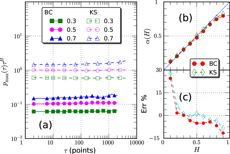
Figure 1: (a) Compensated $p_{\max}(\tau)\tau^{H}$ estimated from fBm simulation with various Hurst numbers $H$ by using box-counting method (denoted as BC) and a kernel smoothing method with Gaussian kernel (denoted as KS), (b) the corresponding scaling exponents $\alpha(H)$, where the theoretical value is illustrated by a solid line, and (c) the relative error $(\alpha-H)/H$ between given and estimated Hurst number. The scaling exponent is estimated on the range $10<\tau<1000$ data points by using a least square fitting algorithm.

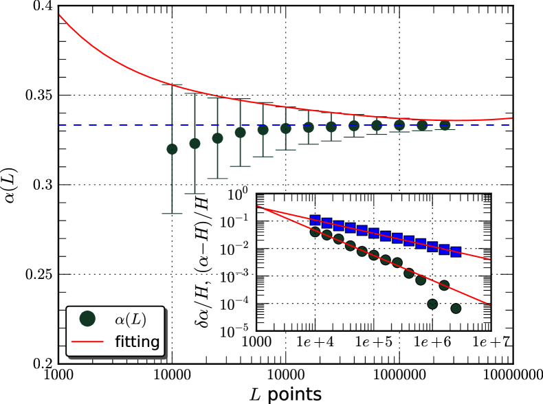
Figure 2: The length dependent $\alpha(L)$ ($\ocircle$) for the Hurst number $H=1/3$ with 1000 realizations (using box-counting method). The horizontal dashed line illustrates the given Hurst number $H=1/3$. The solid line is the fitting of the errorbar (standard deviation of $\alpha(L)$). The inset shows the corresponding relative error $Er(L)=(H-\alpha(L))/H$ ($\ocircle$) and errorbar $\delta\alpha(L)/H$ ($\square$), in which the solid line is the power law fitting $Er(L)\sim L^{-\xi}$ and $\delta\alpha(L)\sim L^{-\gamma}$ with scaling exponents $\xi\simeq 0.91$ and $\gamma\simeq 0.49$ respectively.

II.1 Fractional Brownian motion

FBm is a continuous-time random process proposed by Kolmogorov (1940) in the 1940s and Yaglom (1957) and later named ‘fractional Brownian motion’ by Mandelbrot Mandelbrot and Van Ness (1968). It consists in a fractional integration of a white Gaussian process and is therefore a generalization of Brownian motion, which consists simply in a standard integration of a white Gaussian process. Because it presents deep connections with the concepts of self-similarity, fractal, long-range dependence or $1/f$-process, it quickly became a major tool for various fields where such concepts are relevant, such as in geophysics, hydrology, turbulence, economics, communications, etc. Mandelbrot and Van Ness (1968); Flandrin (1992); Samorodnitsky and Taqqu (1994); Beran (1994); Rogers (1997); Doukhan, Taqqu, and Oppenheim (2003); Gardiner (2004); Biagini et al. (2008); Huang et al. (2009) Below we consider it as an analytical model for monofractal processes to obtain the pdf scaling analytically.

An autocorrelation function of fBm’s increments $Y_{\tau}(t)=x(t+\tau)-x(t)$ is known to be the following

$$R_{\tau}(\ell)=\frac{1}{2}\{(\tau+\ell)^{2H}+|\tau-\ell|^{2H}-\ell^{2H}\}$$ (2)

where $\ell\geq 0$ is the time delay, $\tau$ is the separation scale, and $H$ is Hurst number. Biagini et al. (2008) Thus the standard deviation $\sigma(Y_{\tau})$ of the increment $Y_{\tau}$ scales as

$$\sigma(Y_{\tau})=R_{\tau}(0)^{1/2}=\tau^{H}$$ (3)

$Y_{\tau}$ is also known to have a Gaussian distribution, Mandelbrot and Van Ness (1968); Biagini et al. (2008) which reads as

$$p(Y_{\tau})=\frac{1}{\sigma(Y_{\tau})\sqrt{2\pi}}\exp\left(-\frac{Y_{\tau}^{2}}{2\sigma(Y_{\tau})^{2}}\right)$$ (4)

We thus have a power law relation when $Y_{\tau}=0$

$$p_{\max}(\tau)=p(Y_{\tau})|_{Y_{\tau}=0}=\frac{1}{\sigma(Y_{\tau})\sqrt{2\pi}}=\frac{1}{\sqrt{2\pi}}\tau^{-\alpha(H)}$$ (5)

where $\alpha(H)=H$.

In order to numerically check this, we perform a wavelet based algorithm to simulate the fBm process. Abry and Sellan (1996) We synthesize a segment of length $10^{6}$ data points for each value of Hurst number $H$ from 0.1 to 0.9 by using db2 wavelet. The pdfs are estimated as follows. We first normalize $x$ by its own standard deviation $\sigma$. The empirical pdf is then estimated by using box-counting method on several discrete bins with width $\mathrm{\,d}h$

$$p(Y)=\frac{N_{i}}{N\mathrm{\,d}h}$$ (6)

in which $N_{i}$ is the number of events in the $i$th bin, $N$ is the total length of the data. We find that the empirical pdf $p(Y_{\tau})$, the maxima pdf $p_{\max}(\tau)=\max_{Y_{\tau}}\left\{p(Y_{\tau}|\tau)\right\}$, and the corresponding scaling exponents $\alpha(H)$ are almost independent of the range of bin width $\mathrm{\,d}h$. Another way to estimate the pdf is a kernel smoothing method. Wand and Jones (1995) In this study, a Gaussian kernel is chosen. Figure 1 (a) shows the estimated $p_{\max}(\tau)\tau^{H}$ for various Hurst numbers $H$. For both methods, a clear plateau is observed, indicating power law behavior as expected for all Hurst numbers. We estimate the scaling exponents on the range $10<\tau<1000$ data points by a least square fitting algorithm. The corresponding scaling exponents $\alpha(H)$ are shown in Fig. 1 (b). One can see that, except for the larger values of $H$, the scaling exponents $\alpha(H)$ are in good agreement with the given Hurst numbers. We note that our new method overestimated $H$ for small values of $H$, and then underestimated it for high values. We then check the relative error $(\alpha(H)-H)/H$ between given and estimated Hurst number. The corresponding result is shown in Fig. 1 (c). Generally speaking, both the kernel smoothing method and the box-counting method provide a comparable estimation of $H$, especially for a Hurst number around $H=0.3$. Thus in the following content, we will only apply the box-counting method to real data sets since the scaling exponent is expected around $H=1/3$.

To test the finite length effect, we perform a calculation with various data length $L$ and 1000 realizations each for the Hurst number $H=1/3$, this corresponds to the value for fully developed turbulence. Frisch (1995) The range of $L$ is $10^{4}<L<3\times 10^{6}$. The corresponding scaling exponents $\alpha(L)$ are estimated on the range $10<\tau<1000$ data points. Figure 2 shows $\alpha(L)$ with errorbar $\delta\alpha(L)$, which is the standard deviation of the estimated $\alpha(L)$. The inset shows the relative error $Er(L)=(H-\alpha(L))/H$ ($\ocircle$) and the errorbar $\delta\alpha(L)/H$ ($\square$). Power law behaviors

$$Er(L)\sim(L)^{-\xi},\quad\delta\alpha(L)\sim L^{-\gamma}$$ (7)

are observed with scaling exponents $\xi\simeq 0.91$ and $\gamma\simeq 0.49$. One can find that the estimated $\alpha$ is quickly close to the given Hurst number $H=1/3$. The relative error $Er(L)$ is less than $10\%$ for all $L$ we considered here. Specifically, when $L>10^{5}$, we obtain $Er(L)\leq 1\%$ and $\delta\alpha(L)/H\leq 5\%$. This is already a quite good estimation of $H$. Thus in the following, we choose $L\geq 10^{5}$ data points.

II.2 $H$-Self-similar processes

We can also derive the pdf scaling more generally for $H$-self-similar processes as following. We define a $H$-self-similar process as

$$\left\{x(at)\right\}\stackrel{{\scriptstyle d}}{{=}}\left\{a^{H}x(t)\right\}$$ (8)

in which $\stackrel{{\scriptstyle d}}{{=}}$ means equality in distribution and $H$ is the Hurst number.Embrechts and Maejima (2002) $x(t)$ is a $H$-self-similar process, in which only one parameter $H$, namely Hurst number, is required for the above scaling transform. Let us note $Y_{\tau}=\Delta x_{\tau}=x(t+\tau)-x(t)$, the increment with separation scale $\tau$. We assume that $x$ is $H$-self-similar with stationary increment, hence $Y_{\tau}$ is also $H$-self-similar. Thus one has

$$\left\{\frac{Y_{\tau}}{\tau^{H}}\right\}\stackrel{{\scriptstyle d}}{{=}}\left\{\frac{Y_{T}}{T^{H}}\right\}\stackrel{{\scriptstyle d}}{{=}}\left\{Y_{1}\right\}$$ (9)

In fact equality in distribution means equality for distribution function. Let us write distribution function

$$F(x)=P_{r}(X\leq x)=\int_{-\infty}^{x}p(X)\mathrm{\,d}X$$ (10)

in which $p(x)$ is the pdf of $x$. We note the pdf

$$p(x)=F^{\prime}(x)$$ (11)

We thus take here

$$F_{\tau}(x)=P_{r}\left(Y_{\tau}\leq x\right)$$ (12)

We have

$$P_{r}\left(\frac{Y_{\tau}}{\tau^{H}}\leq x\right)=P_{r}\left(Y_{\tau}\leq x\tau^{H}\right)$$ (13)

Hence Eq. (9) writes for distribution functions

$$F_{\tau}\left(x\tau^{H}\right)=F_{T}\left(xT^{H}\right)$$ (14)

Taking the derivative of Eq. (14), we have for the pdfs

$$\tau^{H}p_{\tau}\left(x\tau^{H}\right)=T^{H}p_{T}\left(xT^{H}\right)$$ (15)

Then writing

$$p_{\max}(\tau)=\max_{x}\left\{p_{\tau}(x)\right\}$$ (16)

and taking the maximum of Eq. (15), we have

$$\tau^{H}p_{\max}(\tau)=T^{H}p_{\max}(T)$$ (17)

Finally, this leads to

$$p_{\max}(\tau)=p_{\max}(T)\left(\tau/T\right)^{-H}$$ (18)

This is the pdf scaling for the $H$-self-similar process. Since Eq. (8) is not true for multi-scaling processes, Eq. (18) may be only an approximation for multifractal processes.

We have shown above analytically the pdf scaling relation for fBm processes and more generally for $H$-self-similar processes. For the former one, the pdf scaling Eq. (1) is validated by numerical simulations. We postulate here that it is also valid for other types scaling time series, e.g. turbulent velocity and temperature from other turbulent systems, etc., and we will check this experimentally in the next section.

The pdf scaling we proposed above is related to the first-order structure function $\alpha=H$ for $H$-self-similar processes, see Eqs. (5) and (18). Hence for the multifractal case, we may postulate that $\alpha=\zeta(1)$, the-first order structure function with a slight intermittent correction, see next section for turbulent velocity as an example.

III Experimental results

In this section, we will apply the above pdf scaling analysis to turbulent velocity obtained from homogeneous and nearly isotropic channel flow, and temperature time series obtained near sidewall area of a Rayleigh-Bénard convection system. An interpretation under the K41 theory is also discussed.

III.1 Turbulent velocity

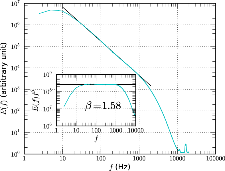
Figure 3: Fourier power spectrum of transverse velocity component at downstream $x/M=48$, where $M$ is the mesh size. The inset shows the corresponding compensated spectra $E(f)f^{\beta}$, where $\beta\simeq 1.58$ is estimated on the range $20<f<1000\,$Hz, corresponding to the time separation $\tau$ on the range $0.001<\tau<0.05\,$s.

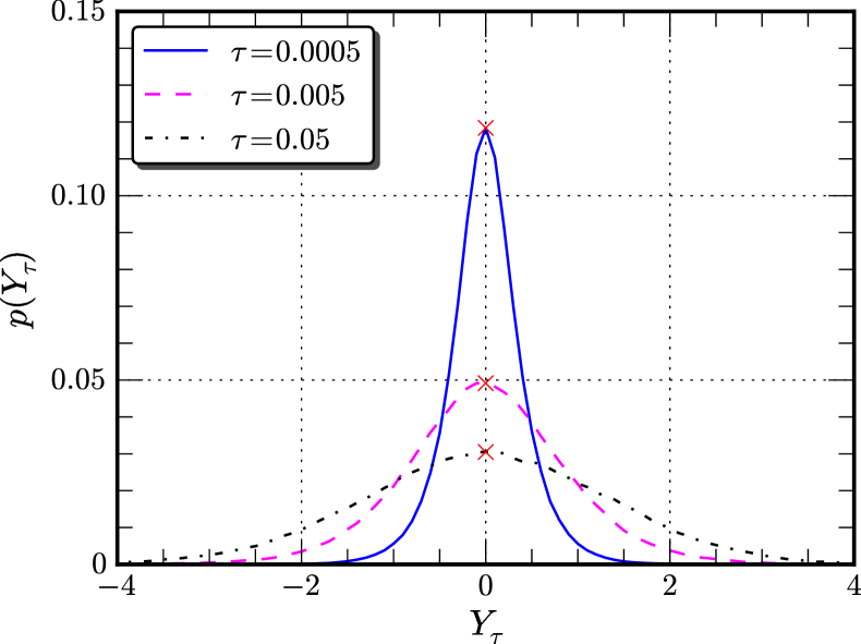
Figure 4: Empirical pdf estimated for transverse velocity with time separation $\tau=0.0005,\,0.005$, and $0.05\,$s, corresponding to $f=2000,\,200$ and $20\,$Hz. The location for $p_{\max}(\tau)$ is marked by $\times$.

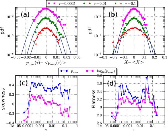
Figure 5: (a) pdf of $p_{\max}(\tau)$, (b) pdf of $X=\log_{10}(p_{\max}(\tau))$, and (c) the skewness factor of $p_{\max}$ (🌑) and $\log_{10}(p_{\max})$, and (d) the flatness factor. Separation scales in (a) and (b) are $\tau=0.0005$ s ($\blacksquare$), $0.01$ s ($\newmoon$) and $\tau=0.1\,$s ($\blacktriangle$), corresponding to $f=2000$ Hz in dissipation range, $100$ Hz in inertial range, and $10$ Hz in large scale forcing range, respectively. For display convenience in (a) and (b), the mean value of each scale is removed and the curves have been vertically shifted. The normal distribution is illustrated by a solid line.

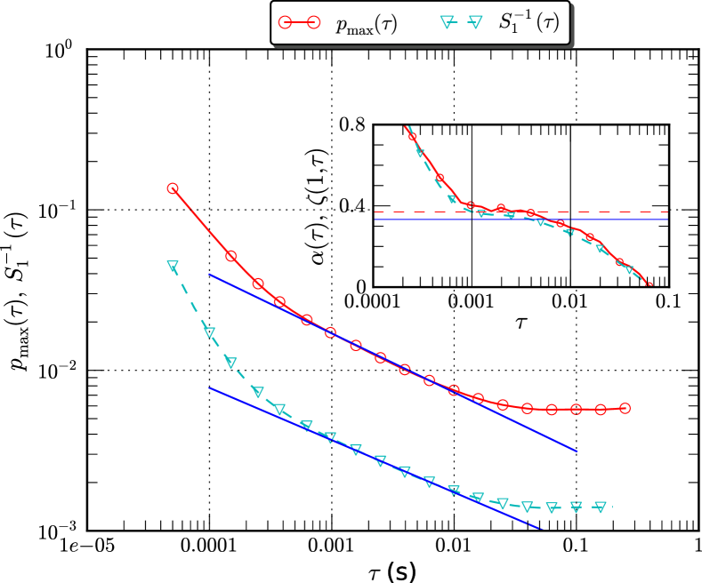
Figure 6: $p_{\max}(\tau)$ and the first-order structure function $S_{1}(\tau)$ of transverse velocity component. The scaling exponents are $\alpha\simeq 0.37$ and $\zeta(1)\simeq 0.34$ estimated on the power law range $0.001<\tau<0.01\,$s, corresponding to $100<f<1000\,$Hz. The inset shows the local slope $\alpha(\tau)$ and $\zeta(1,\tau)$, in which the horizontal solid line indicates the Kolmogorov value $1/3$, and the dashed line indicates the value $0.37$, and the vertical solid line illustrates the inertial range. For display convenience, we have shown the inverse value $1/S_{1}(\tau)$ of the first-order structure function and the curves have been vertically shifted.

We consider here a turbulent velocity database obtained from an experimental homogenous and nearly isotropic turbulent channel flow by using an active-grid technique to achieve a high Reynolds number.Kang, Chester, and Meneveau (2003) We use the data obtained at downstream $x/M=48$, where $M$ is the mesh size. At this measurement location, the mean velocity is $\langle u\rangle=10.8\,$m/s, the turbulence intensity is 10%, and the Taylor microscale based Reynolds number is $Re_{\lambda}\simeq 630$. The sampling frequency is $40,000\,$Hz. To avoid the measurement noise, we only consider here the transverse velocity. Figure 3 shows the Fourier power spectrum for the transverse velocity component. The inset shows the compensated spectrum $E(f)f^{\beta}$, in which $\beta\simeq 1.58$ is the scaling exponent estimated on the range $20<f<1000\,$Hz, corresponding to the time separation $0.001<\tau<0.05\,$s. The value of $\beta$ for transverse velocity component at all measurement locations ($x/M=20,\,30,\,40,\,48$) is around $1.58\sim 1.60$, and is slightly smaller than the Kolmogorov value $5/3$, which could be an effect of the active-grid technique. It demonstrates a nearly two decades inertial range. Thus this database has a long enough inertial range to validate Eq. (1). More details about this database can be found in Ref. Kang, Chester, and Meneveau, 2003.

$p_{\max}(\tau)$ is calculated as explained below. We first divided the time series into several segments with $10^{5}$ data points each. Then empirical pdf is estimated for various separation scales by using Eq. (6). $p_{\max}(\tau)$ is then estimated for each segment. We have $120\times 12=1440$ (number of measurements $\times$ segments of each measurement) realizations. Figure 4 shows the estimated pdf for several separation scales $\tau$ for one realization. The location of maxima pdf $p_{\max}(\tau)$ is marked by $\times$. Graphically, $p_{\max}(\tau)$ decreases with $\tau$ and the corresponding location is around, not exactly, $Y_{\tau}=0$. Figure 5 shows (a) the pdf of $p_{\max}$ for several separation scales $\tau$, (b) $X=\log_{10}(p_{\max})$, (c) the skewness factor of $p_{\max}$ and $\log_{10}(p_{\max})$, and (d) the the flatness factor. The separation scales in Fig. 5 (a) and (b) are $\tau=0.0005$ ($\blacksquare$), $0.01$ ($\newmoon$) and $\tau=0.1\,$s ($\blacktriangle$), corresponding to $f=2000\,$Hz in dissipation range, $100\,$Hz in inertial range and $10\,$Hz in large scale forcing range, respectively. Both normal and lognormal fits seem to capture the fluctuations of $p_{\max}(\tau)$. It seems that the lognormal fit is better than the normal one, but more data are certainly needed to remove measurement uncertainty and to determine without ambiguity which pdf fit is closest to the data.

Figure 6 shows the ensemble averaged $p_{\max}(\tau)$ for the transverse velocity ($\ocircle$). The inset shows the local slope, in which the horizontal solid line illustrates the Kolmogorov value $1/3$ and the dashed line illustrates the value $0.37$, and the vertical solid line demonstrates the plateau range, e.g. the inertial range $0.001<\tau<0.01\,$s. Here the local slope is defined as

$$\alpha(\tau)=-\frac{\mathrm{\,d}\log_{10}(p_{\max}(\tau))}{\mathrm{\,d}\log_{10}(\tau)}$$ (19)

A power law behavior is observed over the range $0.001<\tau<0.01\,$s, corresponding to the frequency range $100<f<1000\,$Hz. This inertial range can be also confirmed by the plateau of the local slope. The scaling exponent is found to be $\alpha\simeq 0.37$, which is obtained by a least square fitting algorithm. It is interesting to note that this value is consistent with the scaling exponent of the first-order SFs reported in other studies, Benzi et al. (1993); She and Lévêque (1994); Arneodo et al. (1996) indicating almost the same intermittent correction on the probability space and the statistical moments space. For comparison, the first-order SF $S_{1}(\tau)=\langle|Y_{\tau}|\rangle$ is also shown as $\triangle$. Note that the absolute value of increments does not change the result of this paper. For display convenience, it has been converted by taking $1/S_{1}(\tau)$. It predicts the same inertial range as $p_{\max}(\tau)$. The corresponding scaling exponent is found to be $\zeta(1)\simeq 0.34$, very close to the Kolmogorov value 1/3. One can find that the $p_{\max}(\tau)$ shows a behavior which seems more linear than $S_{1}(\tau)$ on the inertial range, see also Fig. 7 for temperature data. This is because the first-order SF $S_{1}(\tau)$ is more sensitive to large-scale structures, which might pollute the whole inertial range, see the discussion below and an example of passive scalars with large-scale ramp-cliff structures in Ref. Huang et al., 2010.

We note that the inertial range predicted by Fourier power spectrum $E(f)$ is different from the one predicted by first-order SF $S_{1}(\tau)$ and $p_{\max}(\tau)$. This phenomenon has been reported by several authors for the second-order SF $S_{2}(\tau)$ and the Fourier power spectrum $E(f)$. Nelkin (1994); Frisch (1995); Hou et al. (1998); Huang et al. (2009, 2010) If one considers the Wiener-Khinchin theorem, Percival and Walden (1993); Frisch (1995); Huang et al. (2010) $S_{2}(\tau)$ and $E(f)$ can be related to each other as

$$S_{2}(\tau)=\int_{0}^{+\infty}E(f)\left(1-\cos\left(2\pi\tau f\right)\right)\mathrm{\,d}f$$ (20)

Therefore, for a scaling time series, they are expected to have the same inertial range, and the corresponding scaling exponents are related as $\beta=1+\zeta(2)$. The difference may come from the following reasons: (i) the finite power law range, Hou et al. (1998); Huang et al. (2010) (ii) the spectrum of the original velocity is not a pure power law, Nelkin (1994); Frisch (1995) (iii) violation of the statistical stationary assumption, and (iv) also the influence of large-scale structures. Huang et al. (2010); Huang (2009) More detail of the discussion can be found in Ref. Huang et al., 2010. We will turn to this point again in the next section.

III.2 Temperature as an active scalar from Rayleigh-Bénard Convection

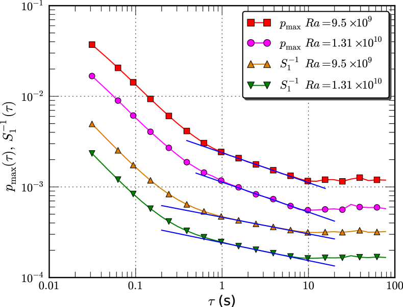
Figure 7: $p_{\max}(\tau)$ and the first-order structure functions $S_{1}^{\theta}(\tau)$ of temperature. Power law behavior is found over the range $1<\tau<10\,$s for all curves. The corresponding scaling exponents are $\alpha_{\theta}\simeq 0.33$ and $\zeta_{\theta}(1)\simeq 0.19$, respectively. For display convenience, we have shown the inverse value $1/S_{1}^{\theta}(\tau)$ of the first-order structure function and the curves have been vertically shifted.

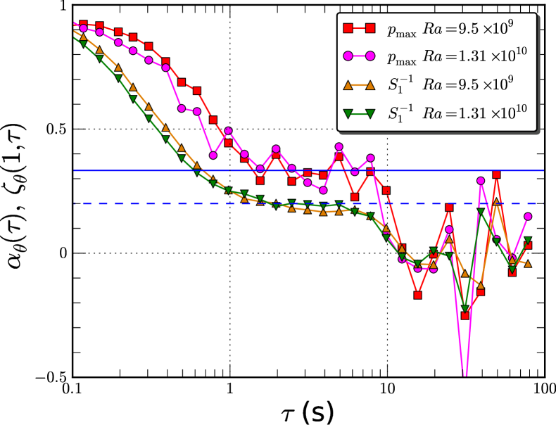
Figure 8: Local slope for the $p_{\max}(\tau)$ and $S^{-1}_{1}(\tau)$. The solid horizontal line is the KOC scaling $1/3$, and the dashed line is the BO59 scaling $1/5$.

We finally consider a temperature data sets obtained near the sidewall of turbulent RBC system. The experiments were performed by Prof. Xia’s group in the Chinese University of Hong Kong. The details of the experiments have been described elsewhere. Shang et al. (2003, 2004); Shang, Tong, and Xia (2008) Briefly, the temperature measurements were carried out in a cylindrical cell with upper and lower copper plates and Plexiglas sidewall. The inner diameter of the cell is $D=19.0$ cm and the height is $L=19.6$ cm. So its aspect ratio is $\Gamma=D/L\simeq 1$. Water was used as the working fluid and measurement were made at Rayleigh number $Ra=9.5\times 10^{9}$ and $1.31\times 10^{10}$. During the experiments, the entire cell was placed inside a thermostat box whose temperature matches the mean temperature of the bulk fluid that was kept at $\sim 40^{\circ}$C, corresponding to a Prandtl number $Pr=4.4$. The local temperature was measured at 8 mm from the sidewall at midheight by using a small thermistor of 0.2 mm diameter and 15 ms time constant. Typically, each measurement of temperature lasted 20 h or longer with a sampling frequency 64 Hz, ensuring that the statistical averaging is adequate.

Near the sidewall of a turbulent convection cell, the turbulent flow is driven by buoyancy in the vertical direction. As proposed by Bolgiano and Obukhov, there is a typical length scale in buoyancy-driven turbulence, now commonly referred to as the Bolgiano scale $L_{B}$, above which buoyancy effects are important and the Bolgiano-Obukhov (BO59) scaling $E_{\theta}(k)\sim k^{-7/5}$ for temperature power spectrum or $S_{q}^{\theta}(r)\sim r^{q/5}$ for SFs are expected. Ahlers, Grossmann, and Lohse (2009); Lohse and Xia (2010) Whether the BO59 scaling exists in turbulent RBC system has been studied extensively in the past two decades, whereas it remains a major challenge to settle this problem (see, for a recent review, Ref. Lohse and Xia, 2010). Nevertheless, it has been shown recently that above a certain scale buoyancy effects indeed become predominant, at least in the time domain. Ching et al. (2004); Zhou and Xia (2008) The observed Bolgiano time scale here is of order 1 second. Zhou and Xia (2001); Ching et al. (2004); Zhou and Xia (2008)

Figure 7 and 8 show respectively the estimated $p_{\max}(\tau)$ and the first-order SFs $S_{1}^{\theta}(\tau)$, and the local slope, in which dashed line indicates the BO59 scaling $1/5$ and the solid line indicates the KOC scaling $1/3$. One can see the power-law behaviors or the plateaus above the Bolgiano time scale, i.e. on the range $1<\tau<10\,$s. For pdfs, the fitted scaling exponent is $\alpha_{\theta}\simeq 0.33$, which is almost the same as the Kolmogorov-Obukhov-Corrsin (KOC) value of $1/3$ for passive scalar,Frisch (1995); Warhaft (2000) whereas for SFs, the fitted scaling exponent $\zeta_{\theta}(1)\simeq 0.19$, which is very close to the BO59 value of $1/5$. At first glance, these results seem to be contradicting and confusing. To understand this, we note that in turbulent RBC buoyant forces are exerted on the fluid mainly via thermal plumes. As revealed by several visualizations, thermal plumes consist of a front with sharp temperature gradient and hence these thermal structures would induce intense temperature increments, which correspond to the pdf tails. Zhang, Childress, and Libchaber (1997); Xi, Lam, and Xia (2004); Zhou, Sun, and Xia (2007) Therefore, it is not surprising that $p_{\max}(\tau)$ investigated here could not capture efficiently the information of thermal plumes and thus may preclude buoyancy effects. See next section for more discussion.

Note that the Taylor’s frozen-flow hypothesis,

$$r_{T}=-\langle u\rangle\tau,$$ (21)

is always used to relate the time domain results, such as those shown in Fig. 7, to the theoretical predictions made for the space domain. However, the conditions for the Taylor’s hypothesis are often not met in turbulent RBC system and hence its applicability to the system is at best doubtful. Sun, Zhou, and Xia (2006); Zhou, Sun, and Xia (2008); Lohse and Xia (2010) Recently, based on a second order approximation, He and coworkers He and Zhang (2006); Zhao and He (2009) advanced an elliptic model for turbulent shear flows. Later, the model was validated in turbulent RBC system indirectly using the temperature data by Tong and coworkers He, He, and Tong (2010); He and Tong (2011) and directly using the velocity data by Zhou et al. (2011). The most important implication of the elliptic model is that the model can be used to translate time series to space series via

$$r_{E}=-(U^{2}+V^{2})^{1/2}\tau$$ (22)

where $U$ is a characteristic convection velocity proportional to the mean velocity and $V$ is a characteristic velocity associated with the r.m.s. velocity and the shear-induced velocity. As pointed by Zhou et al. (2011), $r$ is proportional to $\tau$ for both the Taylor’s relation Eq. (21) and the elliptic relation Eq. (22), but the proportionality constants of the two relations are different. This implies that the Taylor’s hypothesis and elliptic model would yield the same scaling exponents. Therefore, if one is only interested in the scaling exponents, one does not really need the validity of Taylor’s hypothesis to reconstruct the space series from the measured time series.

IV Discussion and Conclusion

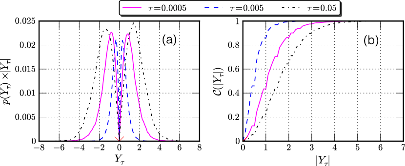
Figure 9: (a) the integral kernel of first-order structure function, and (b) the normalized cumulative function $\mathcal{C}(|Y_{\tau}|)$. The location of $p_{\max}(\tau)$ is at $Y_{\tau}\simeq 0$ and marked by $\times$.

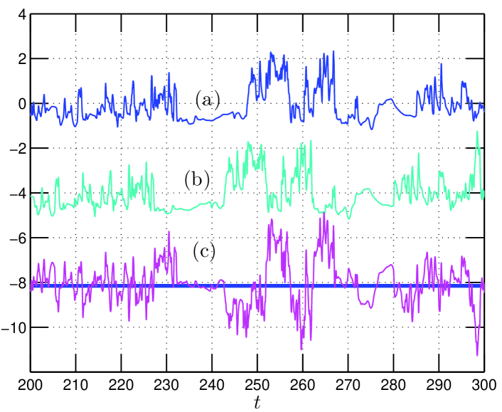
Figure 10: Demonstration of the influence of large-scale structures (plume). They are (a) a portion of temperature data $\theta(t)$, (b) $\theta(t+\tau)$, and (c) increment $Y^{\theta}_{\tau}(t)$ with $\tau=5\,$s, respectively. The $p_{\max}$ is located at $Y^{\theta}_{\tau}\simeq-0.15$, which is indicated by a small horizontal patch. For clarity, the curves have been vertical shifted.

We have mentioned above that for the turbulent velocity the inertial range predicted by Fourier power spectrum $E(f)$ is larger than those predicted by the $p_{\max}(\tau)$ and by the first-order SF. Indeed, it has been reported by several authors that the inertial range predicted by the second-order SF $S_{2}(\tau)$ is shorter than Fourier power spectrum. Nelkin (1994); Frisch (1995); Sreenivasan and Antonia (1997); Hou et al. (1998) By taking an assumption of statistical stationary and Wiener-Khinchin theorem, $S_{2}(\tau)$ and $E(f)$ can be related with each other,Percival and Walden (1993); Frisch (1995) see Eq. (20). Thus both methods are expected to predict an identical inertial range. Frisch (1995); Sreenivasan and Antonia (1997) However, the statement of the Wiener-Khichin theorem only exactly holds for a stationary process, which may be not satisfied by the turbulent velocity.

As pointed by Huang et al. (2010), the second-order SF is also strongly influenced by the large-scale structures. We show this point experimentally here. A more rigorous discussion can be found in Ref. Huang et al., 2010. Figure 9 shows (a) the integral kernel $p(Y_{\tau})\times|Y_{\tau}|$ of the first-order SF for three same separation scales as in Fig. 4 (a), and (b) the corresponding normalized cumulative function $\mathcal{C}(|Y_{\tau}|)$, respectively. The location of $p_{\max}(\tau)$ is marked as $\times$. The normalized cumulative function $\mathcal{C}(|Y_{\tau}|)$ is defined as

$$\mathcal{C}(|Y_{\tau}|)=\frac{\int_{-Y_{\tau}}^{Y_{\tau}}p(Y^{\prime}_{\tau})|Y^{\prime}_{\tau}|\mathrm{\,d}Y^{\prime}_{\tau}}{\int_{-\infty}^{\infty}p(Y^{\prime}_{\tau})|Y^{\prime}_{\tau}|\mathrm{\,d}Y^{\prime}_{\tau}}$$ (23)

It characterizes the relative contribution to the first-order SF. The location of $p_{\max}$ is found graphically to be $Y_{\tau}\simeq 0$, indicating that at this location there is almost no contribution to SFs. If we consider the large index value of $Y_{\tau}$ coming from large-scale structures, most of the contribution to SFs comes from them. The contribution is found also to be increased with the increase of $\tau$, see Fig. 9 (b). Thus $p_{\max}$ is less influenced by large-scale structures, revealing a more accurate scaling exponent for $\zeta(1)$.

In the sidewall region of RBC system, the flow is dominated by plumes. Ahlers, Grossmann, and Lohse (2009); Lohse and Xia (2010) Figure 10 shows (a) a portion of temperature data $\theta(t)$, (b) $\theta(t+\tau)$, and (c) increment $Y^{\theta}_{\tau}$ with $\tau=5\,$s, respectively. Due to the presence of plumes, the shape of pdf $p(Y^{\theta}_{\tau})$ is asymmetric (not shown here). Zhou and Xia (2008) The location of $p_{\max}$ is at $Y^{\theta}_{\tau}\simeq-0.15$, which is indicated as a small horizontal patch. For SFs, they include contribution from all scale structures. On the contrary, $p_{\max}$ acts a kind of conditional statistic, in which the contribution from large-scale structures, e.g. thermal plumes, is excluded, see Fig. 10 (c). The large-scale structures here are believed to be thermal plumes. Thus the scaling of $p_{\max}$ may represent the scaling property of the background fluctuation, which is believed to satisfy KOC scaling. Ahlers, Grossmann, and Lohse (2009); Lohse and Xia (2010) Indeed, the KOC scaling for the first-order statistical moment has been found by using a generalized autocorrelation function of the increment, which confirms the idea that in the sidewall region the temperature fluctuation can be considered as a KOC background fluctuation superposed to BO59 fluctuations (thermal plumes).

This result is compatible with the Grossmann-Lohse (GL) theory,Grossmann and Lohse (2000, 2001, 2002) in which the global thermal dissipation $\epsilon_{\theta}$ is decomposed into the thermal dissipation due to the bulk $\epsilon_{\theta,bulk}$ together with the boundary layer $\epsilon_{\theta,BL}$

$$\epsilon_{\theta}=\epsilon_{\theta,bulk}+\epsilon_{\theta,BL}$$ (24)

Later, the GL theory has been modified so that the thermal dissipation $\epsilon_{\theta}$ can be decomposed into the thermal dissipation due to the thermal plumes $\epsilon_{\theta,pl}$ together with the turbulent background $\epsilon_{\theta,bg}$ Grossmann and Lohse (2004)

$$\epsilon_{\theta}=\epsilon_{\theta,pl}+\epsilon_{\theta,bg}$$ (25)

in which the contribution from the thermal plumes might be related to the boundary layer. Therefore, in the sidewall region, the thermal dissipation is dominated by the thermal plumes (or boundary layer), see more details in Ref. Grossmann and Lohse, 2004. More recently, this picture has been proofed to be correct at least in the central region of the RBC system by Ni, Huang, and Xia (2011). Our result here indicates that in the sidewall region, the turbulent background should have contribution to the global thermal dissipation as well as the thermal plumes. Or in other words, the KOC and BO59 scalings might coexist at least for the temperature fluctuations. We will show this result elsewhere.

The method we proposed here may be refined by considering some pdf models as basis, e.g. Eq. (3.8) in Ref. Castaing, Gagne, and Hopfinger, 1990. However, it seems that the Eq. (3.8) requires the resolution of the spatial dissipation scale $\eta$ to determine a parameter $\sigma_{0}$, the most probable variance of conditional velocity $u$ at a given dissipation rate $\epsilon$, see more details in Ref. Castaing, Gagne, and Hopfinger, 1990. Unfortunately, the data set we have has no resolution on dissipation scale.Kang, Chester, and Meneveau (2003) More data sets and pdf models will be considered in future studies to refine our method.

One advantage of the present method to consider scaling properties of time series is its ability to exclude the influence of large-scale structure as much as possible. Indeed, we have observed a Kolmogorov-like pdf scaling for other data set, in which other moment-based methods do not detect the power-law behavior. It is believed that the scaling is destroyed by large-scale structures (result not shown here).

In summary, we investigated the pdf scaling of velocity increments $Y_{\tau}(t)$. We postulated a scaling relation of the maxima value of the pdfs, e.g. $p_{\max}(\tau)\sim\tau^{-\alpha}$. We obtained this scaling relation analytically for fBm processes and more generally for $H$-self-similar processes with $\alpha=\zeta(1)$. For the former one, it has been validated by fBm simulations. The pdf scaling exponent $\alpha$ is comparable with the scaling exponent $\zeta(1)$ of the first-order SFs. To our knowledge, at least for $H$-self-similar processes, this is the first method to look at scaling properties on the probability space rather than on the statistical moments space as done classically. We postulated that the pdf scaling holds for multifractal processes as well. For multifractal processes, due to the failure of Eq. (8), the scaling relation may be only an approximation.

When applying this approach to turbulent velocity, it is found that, statistically speaking, $p_{\max}(\tau)$ satisfies both normal and lognormal distributions. A scaling exponent $\alpha\simeq 0.37$ is found experimentally which is consistent with the scaling exponent $\zeta(1)$ of the first-order SFs reported in other studies, indicating the same intermittent correction on both the probability space and the statistical moments space. For temperature near the sidewall of RBC system, the scaling exponent is found to be $\alpha_{\theta}\simeq 0.33$. This value is in favor of KOC scaling for passive scalar, not BO59 scaling. It indicates that the KOC scaling may be extracted by a proper designed method. We show experimentally that the contribution of plumes to $p_{\max}$ is almost excluded, whereas the SF contains contributions from both small-scale and larger-scale structures. Indeed the contribution from the former ones is much smaller than from the later ones. Thus the pdf scaling exponent $\alpha_{\theta}$ represents the scaling property of the background flow. In other words, the temperature fluctuation in the side wall region of a RBC can be considered as a KOC background fluctuation superposed to BO59 fluctuations (thermal plumes). The first-order KOC scaling exponent has been confirmed by using other approach. The potential application of these new findings may serve as a constrain of some turbulent models, for example, the pdf model (Eq. (3.8)) in Ref. Castaing, Gagne, and Hopfinger, 1990.