Second order structure function in fully developed turbulence

Abstract

We relate the second order structure function of a time series with the power spectrum of the original variable, taking an assumption of statistical stationarity. With this approach, we find that the structure function is strongly influenced by the large scales. The large scale contribution and the contribution range are respectively 79% and 1.4 decades for a Kolmogorov -5/3 power spectrum. We show numerically that a single scale influence range, over smaller scales is about 2 decades. We argue that the structure function is not a good method to extract the scaling exponents when the data possess large energetic scales. An alternative methodology, the arbitrary order Hilbert spectral analysis which may constrain this influence within 0.3 decade, is proposed to characterize the scaling property directly in an amplitude-frequency space. An analysis of passive scalar (temperature) turbulence time series is presented to show the influence of large scale structures in real turbulence, and the efficiency of the Hilbert-based methodology. The corresponding scaling exponents $\zeta_{\theta}(q)$ provided by the Hilbert-based approach indicate that the passive scalar turbulence field may be less intermittent than what was previously believed.

I Introduction

The most intriguing property of fully developed turbulence is its scale invariance, characterized by a sequence of scaling exponents Kolmogorov (1941); Frisch (1995). Since Kolmogorov’s 1941 milestone work, structure function analysis is widely used to extract these scaling exponents Anselmet et al. (1984); Lepore and Mydlarski (2009); Sreenivasan and Antonia (1997); Lohse and Xia (2010). The second order structure function is written as (we work in temporal space here, through Taylor’s hypothesis)

$$S_{2}(\ell)=\langle\Delta u_{\ell}(t)^{2}\rangle\sim\ell^{\zeta(2)}$$ (1)

where $\Delta u_{\ell}(t)=u(t+\ell)-u(t)$ is the velocity increment, $\ell$ is separation time, and according to K41 theory $\zeta(2)=2/3$ in the inertial range Kolmogorov (1941); Frisch (1995). However, the structure function itself is seldom investigated in detail Bacry et al. (1993); Nichols Pagel et al. (2008). Structure functions have been considered as ‘poor man’s wavelets’ by some authors Bacry et al. (1993). This was mainly linked to a bound in the singularity range that can be grasped by structure functions.

In this paper, we address another issue, the contribution from the large scale structures part and the influence range of a single scale. By taking a statistic stationary assumption and the Wiener-Khinchin theorem Percival and Walden (1993), we relate the second order structure function to the Fourier power spectrum of the original velocity Frisch (1995). We define a cumulative function $\mathcal{P}(f,\ell)$ to characterize the relative contribution of large scale structures, where $\ell$ is the separation scale. It is found that for a pure Kolmogorov 5/3 spectrum the large scale contribution range is more than 1.4 decades and the corresponding relative contribution is about 79%. We show an analysis of experimental homogeneous and nearly isotropic turbulent velocity data base. The compensated spectra provided by different methods show that, due to the influence of large scale structures, the second order structure function predicts a shorter inertial range than other approaches. The cumulative function estimated from the turbulence database shows that the largest contribution of the second order structure function is coming from the large scale part. We then check the influence of a single scale by using fractional Brownian motion (fBm) simulations. We show that the influence range over smaller scales is as large as two decades. We also show that the Hilbert-based methodology Huang et al. (2008a, b); Huang (2009 http://tel.archives-ouvertes.fr/tel-00439605/fr) could constrain this effect within 0.3 decade. We finally analyze a passive scalar (temperature) time series, in which the large scale ‘ramp-cliff’ structures play an important role Sreenivasan (1991); Shraiman and Siggia (2000); Warhaft (2000). Due to the presence of strong ramp-cliff structures, the structure function analysis fails. However, the Hilbert-based approach displays a clear inertial range. The corresponding scaling exponents are quite close to the scaling exponents of longitudinal velocity, indicating a less intermittent passive scalar statistics than what was believed before.

This paper is organized as follows. In section II, we briefly introduce the empirical mode decomposition and arbitrary order Hilbert spectral analysis. By considering Wiener-Khinchin theorem, an analytical model for the second order structure function is proposed in section III. In section IV, analysis results of passive turbulence (temperature) experiment data are presented. We draw the main results and conclusions in section V.

II Arbitrary order Hilbert spectral analysis

Arbitrary order Hilbert spectral analysis is an extended version of the Hilbert-Huang transform (HHT) Huang et al. (1998, 1999). It is designed to characterize scale invariant properties directly in an amplitude-frequency space Huang et al. (2008a, b); Huang (2009 http://tel.archives-ouvertes.fr/tel-00439605/fr). The method possesses two steps: Empirical Mode Decomposition (EMD) and Hilbert spectral analysis. We present a briefly introduction below.

II.1 Empirical Mode Decomposition

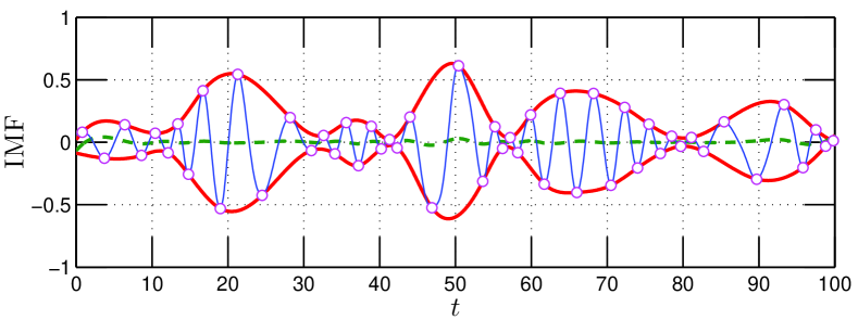
Figure 1: (Color online) An example of IMF from EMD: local extrema points ($\ocircle$), envelope (thick solid line) and running mean (dashed line). It indicates both amplitude and frequency modulations of the Hilbert-based method.

The idea behind EMD is to consider the multi-scale properties of real time series. Then Intrinsic Mode Functions (IMFs) are proposed as mono-scale components. To be an IMF, a function has to satisfy the following two conditions: (i) the difference between the number of local extrema and the number of zero-crossings must be zero or one; (ii) the running mean value of the envelope defined by the local maxima and the envelope defined by the local minima is zero Huang et al. (1998, 1999). Figure 1 shows an example of IMF from EMD, showing both amplitude- and frequency-modulations of Hilbert-based method Huang et al. (1998); Huang (2009 http://tel.archives-ouvertes.fr/tel-00439605/fr). The EMD algorithm, a sifting process, is then designed to decompose a given time series $x(t)$ into a sum of IMF modes $C_{i}(t)$

$$x(t)=\sum_{i=1}^{n}C_{i}(t)+r_{n}(t)$$ (2)

where $r_{n}(t)$ is the residual, which is either a constant or a monotone function Huang et al. (1998, 1999); Rilling et al. (2003). Unlike classical decompositions (Fourier, Wavelet, etc.), there is no basis assumption before the decomposition. In other words, the basis is deduced by the data themselves, which means that this is a completely data-driven method with very local abilities in the physical domain Huang et al. (1998); Flandrin et al. (2004).

II.2 Arbitrary order Hilbert Spectral Analysis

After obtaining the IMF modes, Hilbert transform Cohen (1995); Flandrin (1998) is applied to each IMF

$$\overline{C}_{i}(t)=\frac{1}{\pi}P\int\frac{C_{i}(t^{\prime})}{t-t^{\prime}}\mathrm{\,d}t^{\prime}$$ (3)

where $C_{i}(t)$ is the $i$th IMF mode and $P$ indicates Cauchy principal value. Then the analytical signal is constructed $C^{A}_{i}(t)=C_{i}(t)+j\overline{C}_{i}(t)$. The instantaneous frequency $\omega$ and amplitude $\mathcal{A}$ are estimated by

$$\omega(t)={\color[rgb]{0,0,1}\frac{1}{2\pi}}\frac{\mathrm{\,d}\theta}{\mathrm{\,d}t},\quad\mathcal{A}=\left(C_{i}^{2}(t)+\overline{C}_{i}^{2}(t)\right)^{1/2}$$ (4)

in which $\theta=\arctan\overline{C}_{i}(t)/C_{i}(t)$. Since the Hilbert transform is a singularity integration, the $\omega$ thus have very local ability in spectral space and are free with limitation of the Heisenberg-Gabor uncertainty principle Huang (2005); Cohen (1995); Flandrin (1998). After performing this on all modes series obtained from the analyzed series $x(t)$, one obtains a joint pdf $p(\omega,\mathcal{A})$, which can be extracted from $\omega$ and $\mathcal{A}$ Long et al. (1995); Huang et al. (2008a, b); Huang (2009 http://tel.archives-ouvertes.fr/tel-00439605/fr). The arbitrary order Hilbert marginal spectrum is defined by considering a marginal integration of the joint pdf $p(\omega,\mathcal{A})$, which reads as

$$\mathcal{L}_{q}(\omega)=\int p(\omega,\mathcal{A})\mathcal{A}^{q}\mathrm{\,d}\mathcal{A}$$ (5)

where $q\geq 0$, $\omega$ is the instantaneous frequency, $\mathcal{A}$ the amplitude Huang et al. (2008a, b); Huang (2009 http://tel.archives-ouvertes.fr/tel-00439605/fr). In case of scale invariance, we expect

$$\mathcal{L}_{q}(\omega)\sim\omega^{-\xi(q)}$$ (6)

We have shown elsewhere that $\xi(q)=1+qH$ for fractional Brownian motion, where $H$ is Hurst number Huang et al. (2008a, b); Huang (2009 http://tel.archives-ouvertes.fr/tel-00439605/fr). This generalized Hilbert spectral analysis has been successfully applied to turbulence velocity Huang et al. (2008a), daily river flow discharge Huang et al. (2009a), surf zone Schmitt et al. (2009), etc., to characterize the scale invariance directly in the amplitude-frequency space Huang (2009 http://tel.archives-ouvertes.fr/tel-00439605/fr).

The main drawback of the Hilbert-based methodology is its first step, Empirical Mode Decomposition, which is an algorithm in practice without rigorous mathematical foundation Huang et al. (1998); Huang (2005). Flandrin and his co-workers have obtained some theoretical results on the EMD method Flandrin et al. (2004); Rilling and Flandrin (2006, 2008, 2009). However, more theoretical work is still needed to fully mathematically understand this method.

III second order structure function

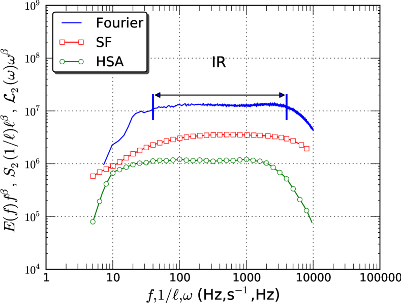
Figure 2: (Color online) Compensated spectra of transverse velocity. A plateau is observed on the range $40<f<4000$ Hz for Fourier spectrum (solid line) and $20<f<2000$ Hz for Hilbert spectrum ($\ocircle$), respectively. For comparison, the compensated spectra for the second order structure function ($\square$) is also shown. The compensated values $\beta$ are estimated case by case. For display convenience, the curves have been vertically shifted.

$f$ (Hz)	0.01	0.04	0.1	0.2	0.5	1	10	100
$\mathcal{P}$ (%)	0.46	2.95	9.91	24.0	62.7	78.6	95.3	99.0
$\mathcal{Q}$ (%)	-2.3	-14.1	-44.4	-83.5	1.8	49.0	88.5	97.6

Table 1: Index values of analytical expressions $\mathcal{P}(f,1)$ and $\mathcal{Q}(f,1)$ with $\beta=5/3$ for several frequencies.

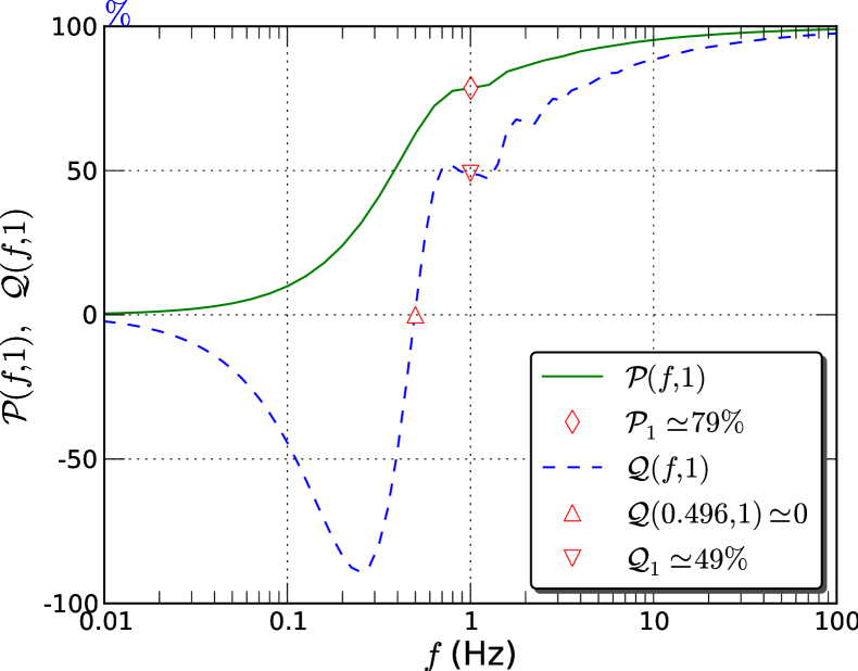
Figure 3: (Color online) Semilog plot of analytical expressions of $\mathcal{P}(f,1)$ (solid line) and $\mathcal{Q}(f,1)$ (dashed line) with $\beta=5/3$ on the range $0.01<f<100$ Hz. Symbols are respectively the index values of $\mathcal{P}_{1}(1)\simeq 79\%$ ($\diamondsuit$), the large scales part contribution to the second order structure function, $\mathcal{Q}(0.496,1)\simeq 0$ ($\triangle$), the zero-crossing point of the autocorrelation function, and $\mathcal{Q}_{1}(1)\simeq 49\%$ ($\triangledown$), the large scales part contribution to the autocorrelation function, see also Table 1.

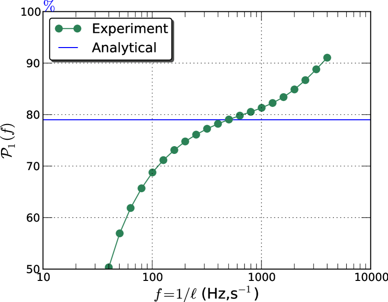
Figure 4: (Color online) Cumulative function $\mathcal{P}_{1}(f)$ estimated from turbulent experimental data for transverse velocity on the inertial range $40<f<4000\,$Hz. The analytical expression for $\mathcal{P}$ shows $\mathcal{P}_{1}\simeq 79\%$ (horizontal solid line). We note that all $\mathcal{P}_{1}\geq 50\%$, which means that most contribution of the second order structure function comes from the large scales part $f<1/\ell$.

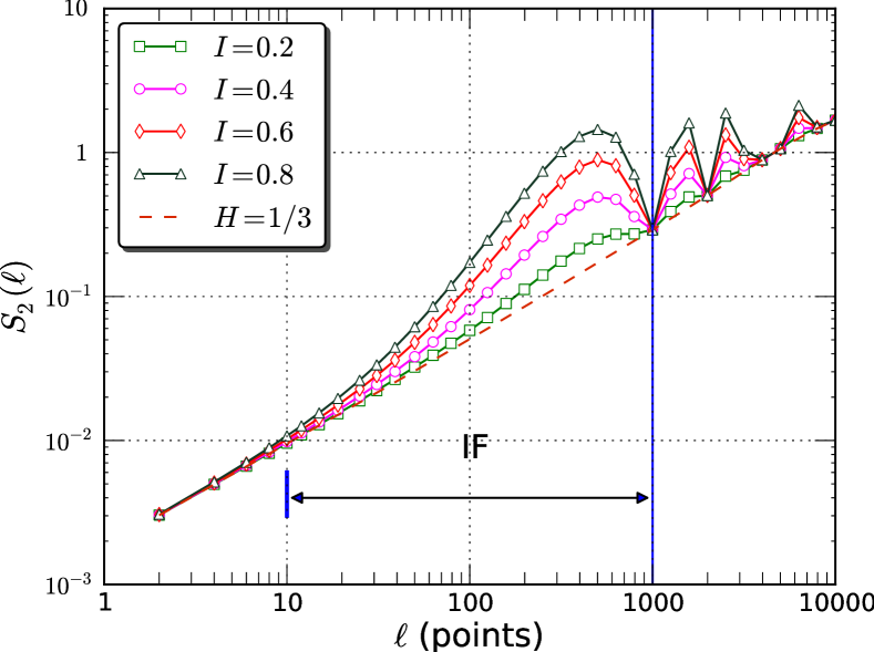
Figure 5: (Color online) Periodic effect on the second order structure function with various intensities $I$, where the vertical line illustrates the location of the perturbation sine wave.

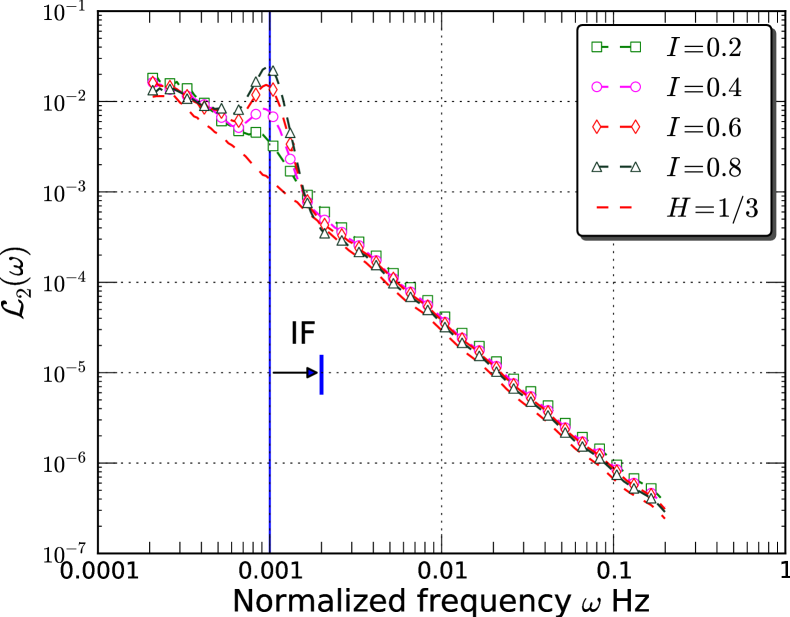
Figure 6: (Color online) Periodic effect on the second order Hilbert marginal spectrum with various intensities $I$, where the vertical line illustrates the location of the perturbation sine wave.

The structure function is the most widely used method in turbulence research to extract the scaling exponents Monin and Yaglom (1971); Anselmet et al. (1984); Frisch (1995); Sreenivasan and Antonia (1997); Lepore and Mydlarski (2009); Lohse and Xia (2010). It has also been used in may other fields to characterize the scale invariance properties of time series, e.g. climate data Schmitt et al. (1995), financial research Schmitt et al. (1999), to quote a few. The relationship between the second order structure function and the corresponding Fourier power spectrum has been investigated previously by Lohse and Müller-Groeling Lohse and Müller-Groeling (1995, 1996). They obtained an analytical expression of Fourier power spectrum for turbulent velocity by considering a Batchelor fit for the second order structure functions. They found that the energy pileups at the ends of scaling ranges in Fourier space, which leads to a bottleneck effect in turbulence. Here we focus on another aspect of the second order structure function, the scale contribution and contribution range from the large scale part.

Considering a statistical stationary assumption and the Wiener-Khinchin theorem Percival and Walden (1993), we can relate the second order structure function to the Fourier power spectrum of the original velocity Frisch (1995)

$$S_{2}(\ell)=\langle\Delta u(\ell)^{2}\rangle=\int_{0}^{+\infty}E_{u}(f)(1-\cos(2\pi f\ell))\mathrm{\,d}f$$ (7)

where we neglect a constant in front of the integral, and $E_{u}(f)$ is the Fourier power spectrum of the velocity. Let us introduce a cumulative function

$$\mathcal{P}(f,\ell)=\frac{\int_{0}^{f}E_{u}(f^{\prime})(1-\cos(2\pi f^{\prime}\ell))\mathrm{\,d}f^{\prime}}{\int_{0}^{+\infty}E_{u}(f^{\prime})(1-\cos(2\pi f^{\prime}\ell))\mathrm{\,d}f^{\prime}}\times 100\%$$ (8)

$\mathcal{P}(f,\ell)$ is increasing from 0 to 1, and measures the relative contribution to the second order structure function from 0 to $f$. We are particular concerned by the case $f=1/\ell$, $\mathcal{P}_{1}(f)=\mathcal{P}(f,\ell)|_{f=1/\ell}$, which measures the relative contribution from large scales. If we assume a power law for the spectrum

$$E_{u}(f)=cf^{-\beta},\,c>0$$ (9)

when substituted into Eq. (7), this gives a divergent integral for some values of $\beta$. The convergence condition requires $1<\beta<3$ Frisch (1995). In the appendix, we derive an analytical expression for $S_{2}(\ell)$

$$S_{2}(\ell)=\frac{c\pi^{\beta-\frac{1}{2}}\,\Gamma(\frac{3}{2}-\frac{\beta}{2})}{(\beta-1)\,\Gamma(\frac{\beta}{2})}\ell^{\beta-1}$$ (10)

and for $\mathcal{P}(f,\ell)$

$$\mathcal{P}(f,\ell)=\frac{1}{a(\beta)}\bigg{\{}(3-\beta)(\cos(f)-1)f^{1-\beta}+g(f,\beta)\,f^{3-\beta}\bigg{\}}\times 100\%$$ (11)

in which $a(\beta)=\sqrt{\pi}\,(3-\beta)\,2^{1-\beta}\,\Gamma(3/2-\beta/2)\Gamma(\beta/2)^{-1}$, and $g(f,\beta)={}_{1}F_{2}(3/2-\beta/2,3/2,5/2-\beta/2,-f^{2}/4)$ is a generalized hypergeometric function Abramowitz and Stegun (1970). For fully developed turbulence, the Kolmogorov spectrum corresponds to $\beta=5/3$ Kolmogorov (1941); Frisch (1995).

We apply here the above approach to a database from an experimental homogeneous and nearly isotropic turbulent channel flow at downstream $x/M=20$, where $M$ is the mesh size. The flow is characterized by a Taylor microscale based Reynolds number $Re_{\lambda}=720$ and the sampling frequency is $f_{s}=40,000\,$Hz Kang et al. (2003). The detail of this experiment can be found in Ref. Kang et al. (2003). Figure 2 shows the compensated spectra for transverse velocity components on the range $5<f<10,000\,$Hz, in which the spectra are estimated by Fourier analysis (solid line) Kang et al. (2003), the second order structure function ($\square$), and the arbitrary order Hilbert spectral analysis ($\ocircle$) Huang et al. (2008a); Huang (2009 http://tel.archives-ouvertes.fr/tel-00439605/fr), respectively. The compensated values $\beta$ are estimated case by case. For comparison convenience, we represent the structure function as a function of $f=1/\ell$. Except for the structure function, there is a plateau which is more than two decades wide. We also note that the curves provided by second order structure function and the Fourier power spectrum are not identical with each other, which is required by Eq. (7). This has been reported by several authors Frisch (1995); Hou et al. (1998); Nelkin (1994). The difference may come from the finite scaling range Nelkin (1994); Hou et al. (1998) and also violation of the statistical stationary assumption Huang (2009 http://tel.archives-ouvertes.fr/tel-00439605/fr).

We note that $\mathcal{P}(f,\ell)$ is independent of $\ell$ since we assume a pure power law relation (9), see the appendix for more detail. Below we only consider the case $\ell=1\,$s, e.g. $\mathcal{P}(f,1)$. We concentrate on the large scales ($f<1$ Hz) contribution to the second order structrue function, e.g. $\mathcal{P}_{1}(1)=\mathcal{P}(f,1)|_{f=1}$, which measures the contribution from large scales. Figure 3 and Table 1 show respectively the analytical curve $\mathcal{P}(f,1)$ and various index values on the range $0.01<f<100$ Hz for a pure Kolmogorov power law by taking $\beta=5/3$. The contribution from the large scales part ($f<1$ Hz) is 79% ($\diamondsuit$), see Table 1. The contribution from the first decade large scales, $0.1<f<1$ Hz, is about 69%. For the second decade, $0.01<f<0.1$ Hz, the contribution is about 9.5%. The large scale contribution range of the second order structure function is more than 1.4 decades if we neglect the 3% contribution from $f<0.04$ Hz, see Table 1. We have given elsewhere an analytical model for the autocorrelation function of velocity increments based on the same idea Huang et al. (2009b). It writes as

$$R(\ell,\tau)=\int_{0}^{\infty}E_{u}(f)(1-\cos(2\pi f\ell))\cos(2\pi f\tau)\mathrm{\,d}f$$ (12)

in which $\ell$ is the separation time and $\tau$ is the time delay Huang et al. (2009b). We are particularly concerned with the case $\tau=\ell$, in which $R(\ell,\tau)$ takes its minimum value Huang et al. (2009b). Power law behavior is found as $R(\ell,\tau)|_{\tau=\ell}\sim\ell^{\beta-1}$ if one substitutes Eq. (9) into the above equation. The corresponding cumulative function reads as

$$\mathcal{Q}(f,\ell)=\frac{\int_{0}^{f}E_{u}(f^{\prime})(1-\cos(2\pi f^{\prime}\ell))\cos(2\pi f^{\prime}\ell)\mathrm{\,d}f^{\prime}}{\int_{0}^{\infty}E_{u}(f^{\prime})(1-\cos(2\pi f^{\prime}\ell))\cos(2\pi f^{\prime}\ell)\mathrm{\,d}f^{\prime}}\times 100\%$$ (13)

Again, assuming the pure power law of Eq. (9), we have an analytical expression for the above equation, see Eq. (20) in the Appendix.

For comparison, the analytical expression $\mathcal{Q}$ with $\beta=5/3$ is also shown as a dashed line in Fig. 3. We note that $\mathcal{Q}$ crosses zero at $f\simeq 0.496$ Hz ($\triangle$), see also Table 1, which indicates that at this position, contributions from large scales $f\lesssim 0.5$ Hz are vanishing (canceled by themselves). It indicates that the large scale contribution range is about 0.3 decade, e.g. $0.496<f<1$ Hz, and the contribution itself is found to be 49%, see Table 1. This explains why the minimum value of the autocorrelation function of the velocity increments is a better indicator of the inertial range than structure functions Huang et al. (2009b). The corresponding $\mathcal{P}_{1}=\mathcal{P}(f,\ell)|_{f=1/\ell}$ based on $E_{u}(f)$ from the experimental data are shown in Fig. 4 for transverse velocity on the range $40<f<4000\,$Hz, which is the inertial range predicted by Fourier power spectrum, see Fig. 2. The analytical value of $\mathcal{P}_{1}(1)\simeq 79\%$ provided by Eq. (11) is shown as a solid line. Below this line, the second order structure function is influenced by both the finite length of power law and, more importantly, large scale structures, see next paragraph. Above this line, it is thus influenced by the finite length of the power law (or viscosity). The index value of $\mathcal{P}_{1}$ is significantly larger than 50%, showing that the largest contribution of the second order structure function is coming from the large scale part.

We then consider the influence of a single scale. We simulate a fBm time series $x(t)$ with Hurst number $H=1/3$, corresponding to the Hurst value of turbulent velocity. A sine wave is superposed to the normalized fBm data with frequency $f_{0}=0.001$ Hz and various intensities $I$: $x(t)=x(t)/\textrm{Var}(x)+I\sin(2\pi f_{0}t)$. We then perform structure function analysis and Hilbert spectral analysis on these data. Figure 5 shows the second order structure function. It is strongly influenced by the periodic component Huang et al. (2008a). The influence range down to the small scale is as large as 2 decades. It indicates that the structure functions is strongly influenced by a large energetic scale structures, e.g. coherent structures. Figure 6 shows the corresponding second order Hilbert marginal spectrum where the influence down to the small scale is constrained within 0.3 decade. It might be linked to the fact that the first step of the arbitrary order Hilbert spectral analysis, the empirical mode decomposition, acts a dyadic filter bank for several types of time series Huang et al. (2008a); Flandrin et al. (2004); Wu and Huang (2004).

IV Passive scalar turbulence

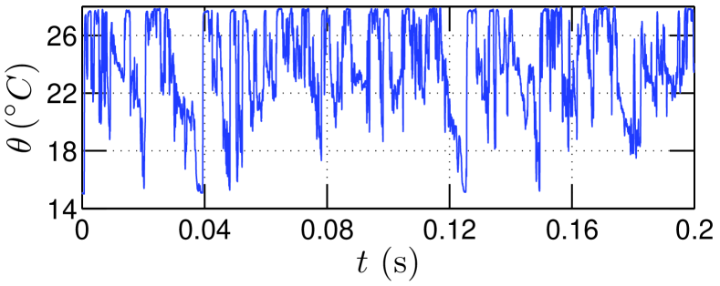
Figure 7: A 0.2s portion of the temperature time series, showing strong ramp-cliff structures.

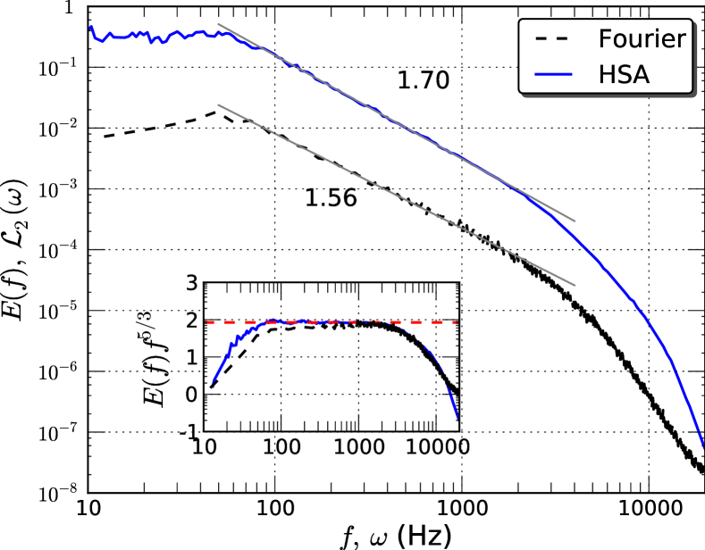
Figure 8: (Color online) Fourier power spectrum and Hilbert marginal spectrum for temperature. Compensated spectra by $f^{5/3}$ are shown as inset. Both methods predict power law behavior on the range $80<f<2000\,$Hz. For display convenience, the curves have been vertical shifted.

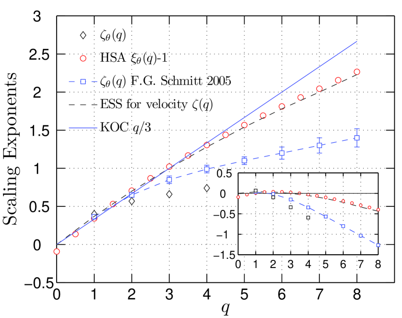
Figure 9: (Color online) Scaling exponents for passive scalar, which is estimated by Hilbert-based approach $\xi_{\theta}(q)-1$ ($\ocircle$), and the structure functions $\zeta_{\theta}(q)$ ($\diamondsuit$). For comparison, the scaling exponents compiled by Schmitt (2005) ($\square$) for passive scalar, and compiled by Arneodo et al. (1996) for the velocity (dashed-line) are also shown.

The above arguments and results indicate that the structure functions are strongly influenced by the large scales and that this approach is not a good methodology to extract the scaling exponents when the data possess large energetic scale structures. This is the case of scalar turbulence: ramp-cliff structures are an important signature of the passive scalar Sreenivasan (1991); Shraiman and Siggia (2000); Warhaft (2000); Celani et al. (2000). To consider this experimentally, we analyze here a temperature time series obtained in a shear layer between a jet flow and a cross flow. The bulk Reynolds number is about $Re=60000$. The initial temperature of the two flows are $T_{J}=27.8^{\circ}C$ and $T=14.8^{\circ}C$. The measurement location is close to the nozzle of the jet. Figure 7 shows a 0.2s portion temperature data, illustrating strong ramp-cliff structures.

Figure 8 shows the Fourier power spectrum (dashed line) and Hilbert marginal spectrum (solid line), where the inset shows the compensated spectra by $f^{5/3}$. Both methods predict a more than 1.4 decades power law behavior on the range $80<f<2000\,$Hz. However, the Fourier analysis requires high order harmonic components to represent the ramp-cliff structures. It leads to an artificial energy transfer from low frequencies (large scales) to high frequencies (small scales) in Fourier space, causing a less steep spectrum Huang et al. (1998); Huang (2009 http://tel.archives-ouvertes.fr/tel-00439605/fr). Since both EMD and Hilbert spectral analysis have a very local ability, the effect of ramp-cliff structures is constrained.

Due to the presence of ramp-cliff structures, the structure function analysis fails (figure not shown here, see Ref. Huang (2009 http://tel.archives-ouvertes.fr/tel-00439605/fr)). However, the Hilbert-based methodology shows a clear inertial range also for other moment orders, up to $q=8$ (not shown here). Figure 9 shows the scaling exponents provided by Hilbert-based approach $\xi_{\theta}(q)-1$ ($\ocircle$). For comparison, the scaling exponents directly estimated by structure functions $\zeta_{\theta}(q)$ ($\diamondsuit$), the scaling exponents $\zeta_{\theta}(q)$ ($\square$) compiled by Schmitt (2005) for passive scalar, and the ESS scaling exponents $\zeta(q)$ (dashed line) for velocity Arneodo et al. (1996). Due to the effect of ramp-cliff structures, the scaling exponents provided directly by the structure functions seem to saturate when $q>2$. The scaling exponents $\xi_{\theta}(q)-1$ provided by the Hilbert-based methodology are quite close to the ESS for the longitudinal velocity Arneodo et al. (1996), indicating a less intermittent scalar field than what was believed before. We must underline here that the Hilbert-based approach provided the same exponents as the structure function for the velocity field Huang et al. (2008a) when there is no large scale energetic forcing. The difference found here for the passive scalar case may thus come from the fact that temperature fluctuations have a strong large scale contribution. Apparently the ramp-cliff structure is a large scale of the order of an integral scale Sreenivasan (1991). The cliff is sharp, and thus is manifested at the small scales: this may be interpreted as a coupling between the large ramp-cliff structures and the small scales Sreenivasan (1991). As we argued above, the inertial range, if it exists, is strongly influenced by the these large scale structures.

V Discussion and summary

In summary, based on an assumption of statistical stationarity, we investigated here an analytic model of the second order structure function. By introducing a cumulative function, we have found that the structure function is strongly influenced by the large scales. The large scale contribution range is found as being 1.4 decades wide and the contribution is about 79%. We have shown numerically that the single scale influence range down to the small scale is as large as 2 decades. The Hilbert-based methodology may constrain the large scale effect to 0.3 decade. We then showed an analysis from a passive scalar time series with strong ramp-cliff structures, in which the classical structure functions fail. Surprisingly, the scaling exponents predicted by Hilbert-based approach are almost the same as the scaling exponents for longitudinal velocity in fully developed turbulence, indicating a less intermittent passive scalar statistics than what was believed before.

This should be verified using more databases, but it may be giving an explanation to the question open for a long time, of why passive scalars, being passive quantities, are more intermittent than the velocity field. We hope that the result obtained here can contribute to reconsidering the statistical properties of turbulence with large energetic scale structures.

Appendix A Analytical expression of the second order structure functions

In this Appendix, we show hot to obtain the analytical expressions (10) and (11) for the second order structure functions and its cumulative function (8), respectively, for a scaling power law spectrum given by Eq. (9).

We substitute Eq. (9) into Eq. (7)

$$S_{2}(\ell)=\int_{0}^{\infty}cf^{-\beta}(1-\cos(2\pi f\ell))\mathrm{\,d}f$$ (14)

After a scaling transform $f^{\prime}=2\pi\ell f$, we have

$$S_{2}(\ell)=(2\pi\ell)^{\beta-1}\int_{0}^{\infty}cf^{\prime-\beta}(1-\cos(f^{\prime}))\mathrm{\,d}f^{\prime}$$ (15)

We rewrite the integration range from $0$ to $f$

$$S_{2}(\ell,f)=(2\pi\ell)^{\beta-1}\int_{0}^{f}cx^{-\beta}\left(1-\cos(x)\right)\mathrm{\,d}x$$ (16)

By applying integration by parts, we have

$$\begin{array}[]{lll}S_{2}(\ell,f)&=\frac{c(2\pi\ell)^{\beta-1}}{1-\beta}\bigg{\{}\underbrace{x^{1-\beta}(1-\cos(x))}_{A}|_{0}^{f}\\ &-\underbrace{\int_{0}^{f}x^{1-\beta}\sin(x)\mathrm{\,d}x}_{B}\bigg{\}}\end{array}$$ (17)

where $1<\beta<3$. It is not difficult to show that $\lim_{f\to 0}A=0$. An analytical expression for $B$ is

$$B={}_{1}F_{2}(3/2-\beta/2,3/2,5/2-\beta/2,-f^{2}/4)$$ (18)

in which ${}_{1}F_{2}$ is a generalized hypergeometric function Abramowitz and Stegun (1970). In the limit $f\to\infty$, we have

$$\lim_{f\to\infty}A=0,\,\lim_{f\to\infty}B=\frac{\sqrt{\pi}\,\Gamma(\frac{3}{2}-\frac{\beta}{2})}{2^{\beta-1}\,\Gamma(\frac{\beta}{2})}$$ (19)

We finally obtain Eq. (10) and (11).

The analytical expression for $\mathcal{Q}$ can be obtained by the same procedure, which reads as

$$\mathcal{Q}(f,\ell)=\frac{1}{b(\beta)}\bigg{\{}(3-\beta)(\cos(f)-1)\cos(f)f^{1-\beta}+\,h(f,\beta)\,f^{3-\beta}\bigg{\}}\times 100\%$$ (20)

in which $b(\beta)=-\sqrt{\pi}\,(3-\beta)\,(2^{1-\beta}-1/2)\,\Gamma(3/2-\beta/2)\Gamma(\beta/2)^{-1}$, and $g(f,\beta)=2\,{}_{1}F_{2}\big{(}{3}/{2}$ $-{\beta}/{2},{3}/{2},{5}/{2}-{\beta}/{2},-f^{2}\big{)}-{}_{1}F_{2}\!\left({3}/{2}-{\beta}/{2},{3}/{2},{5}/{2}-{\beta}/{2},-{f^{2}}/{4}\right)$, and ${}_{1}F_{2}$ is again a generalized hypergeometric function. It is also independent of $\ell$.

References

- Kolmogorov (1941) A. N. Kolmogorov, Dokl. Akad. Nauk SSSR 30, 299 (1941).
- Frisch (1995) U. Frisch, Turbulence: the legacy of AN Kolmogorov (Cambridge University Press, 1995).
- Anselmet et al. (1984) F. Anselmet, Y. Gagne, E. J. Hopfinger, and R. A. Antonia, J. Fluid Mech. 140, 63 (1984).
- Lepore and Mydlarski (2009) L. Lepore and L. Mydlarski, Phy. Rev. Lett. 103, 034501 (2009).
- Sreenivasan and Antonia (1997) K. Sreenivasan and R. Antonia, Annu. Rev. Fluid Mech. 29, 435 (1997).
- Lohse and Xia (2010) D. Lohse and K.-Q. Xia, Ann. Rev. Fluid Mech. 42, 335 (2010).
- Bacry et al. (1993) E. Bacry, J. Muzy, and A. Arneodo, J. Statist. Phys. 70, 635 (1993).
- Nichols Pagel et al. (2008) G. Nichols Pagel, D. Percival, P. Reinhall, and J. Riley, Physica D 237, 665 (2008).
- Percival and Walden (1993) D. Percival and A. Walden, Spectral Analysis for Physical Applications: Multitaper and Conventional Univariate Techniques (Cambridge University Press, 1993).
- Huang et al. (2008a) Y. Huang, F. G. Schmitt, Z. Lu, and Y. Liu, Europhys. Lett. 84, 40010 (2008a).
- Huang et al. (2008b) Y. Huang, F. G. Schmitt, Z. Lu, and Y. Liu, Traitement du Signal 25, 481 (2008b).
- Huang (2009 http://tel.archives-ouvertes.fr/tel-00439605/fr) Y. Huang, Ph.D. thesis, Université des Sciences et Technologies de Lille - Lille 1, France & Shanghai University, China (2009) http://tel.archives-ouvertes.fr/tel-00439605/fr.
- Sreenivasan (1991) K. Sreenivasan, Proc. R. Soc. Lond. A 434, 165 (1991).
- Shraiman and Siggia (2000) B. Shraiman and E. Siggia, Nature 405, 639 (2000).
- Warhaft (2000) Z. Warhaft, Annu. Rev. Fluid Mech. 32, 203 (2000).
- Huang et al. (1998) N. E. Huang, Z. Shen, S. R. Long, M. C. Wu, H. H. Shih, Q. Zheng, N. Yen, C. C. Tung, and H. H. Liu, Proc. R. Soc. London, Ser. A 454, 903 (1998).
- Huang et al. (1999) N. E. Huang, Z. Shen, and S. R. Long, Annu. Rev. Fluid Mech. 31, 417 (1999).
- Rilling et al. (2003) G. Rilling, P. Flandrin, and P. Gonçalvès, IEEE-EURASIP Workshop on Nonlinear Signal and Image Processing (2003).
- Flandrin et al. (2004) P. Flandrin, G. Rilling, and P. Gonçalvès, IEEE Sig. Proc. Lett. 11, 112 (2004).
- Cohen (1995) L. Cohen, Time-frequency analysis (Prentice Hall PTR Englewood Cliffs, NJ, 1995).
- Flandrin (1998) P. Flandrin, Time-frequency/time-scale analysis (Academic Press, 1998).
- Huang (2005) N. E. Huang, Hilbert-Huang Transform and Its Applications (World Scientific, 2005), chap. 1. Introduction to the Hilbert-Huang transform and its related mathematical problems, pp. 1–26.
- Long et al. (1995) S. R. Long, N. E. Huang, C. C. Tung, M. L. Wu, R. Q. Lin, E. Mollo-Christensen, and Y. Yuan, IEEE Geoscience and Remote Sensing Soc. Lett. 3, 6 (1995).
- Huang et al. (2009a) Y. Huang, F. G. Schmitt, Z. Lu, and Y. Liu, J. Hydrol. 373, 103 (2009a).
- Schmitt et al. (2009) F. G. Schmitt, Y. Huang, Z. Lu, L. Y., and N. Fernandez, J. Mar. Sys. 77, 473 (2009).
- Rilling and Flandrin (2006) G. Rilling and P. Flandrin, IEEE International Conference on Acoustics, Speech and Signal Processing, 2006. ICASSP 2006 Proceedings. 2006 3, 444 (2006).
- Rilling and Flandrin (2008) G. Rilling and P. Flandrin, IEEE Trans. Signal Process (2008).
- Rilling and Flandrin (2009) G. Rilling and P. Flandrin, Adv. Adapt. Data Anal. 1, 43 (2009).
- Monin and Yaglom (1971) A. S. Monin and A. M. Yaglom, Statistical fluid mechanics vd II (MIT Press Cambridge, Mass, 1971).
- Schmitt et al. (1995) F. G. Schmitt, S. Lovejoy, and D. Schertzer, Geophys. Res. Lett. 22, 1689 (1995).
- Schmitt et al. (1999) F. G. Schmitt, D. Schertzer, and S. Lovejoy, Appl. Stoch. Models and Data Anal. 15, 29 (1999).
- Lohse and Müller-Groeling (1995) D. Lohse and A. Müller-Groeling, Phys. Rev. Lett. 74, 1747s (1995).
- Lohse and Müller-Groeling (1996) D. Lohse and A. Müller-Groeling, Phys. Rev. E 54, 395 (1996).
- Abramowitz and Stegun (1970) M. Abramowitz and I. A. Stegun, Handbook of Mathematical Functions (Dover, New York, 1970).
- Kang et al. (2003) H. Kang, S. Chester, and C. Meneveau, J. Fluid Mech. 480, 129 (2003).
- Hou et al. (1998) T. Hou, X. Wu, S. Chen, and Y. Zhou, Phys. Rev. E 58, 5841 (1998).
- Nelkin (1994) M. Nelkin, Adv. Phys. 43, 143 (1994).
- Huang et al. (2009b) Y. Huang, F. G. Schmitt, Z. Lu, and Y. Liu, Europhys. Lett. 86, 40010 (2009b).
- Wu and Huang (2004) Z. Wu and N. E. Huang, Proc. R. Soc. London, Ser. A 460, 1597 (2004).
- Schmitt (2005) F. G. Schmitt, Eur. Phys. J. B 48, 129 (2005).
- Arneodo et al. (1996) A. Arneodo, C. Baudet, F. Belin, R. Benzi, B. Castaing, B. Chabaud, R. Chavarria, S. Ciliberto, R. Camussi, and F. Chilla, Europhys. Lett. 34, 411 (1996).
- Celani et al. (2000) A. Celani, A. Lanotte, A. Mazzino, and V. M., Phys. Rev. Lett. 84, 2385 (2000).
- Celani et al. (2000) http://www.me.jhu.edu/~meneveau/datasets.html.