Quantum probes for fractional Gaussian processes

Abstract

We address the characterization of classical fractional random noise via quantum probes. In particular, we focus on estimation and discrimination problems involving the fractal dimension of the trajectories of a system subject to fractional Brownian noise. We assume that the classical degree of freedom exposed to the environmental noise is coupled to a quantum degree of freedom of the same system, e.g. its spin, and exploit quantum limited measurements on the spin part to characterize the classical fractional noise. More generally, our approach may be applied to any two-level system subject to dephasing perturbations described by fractional Brownian noise, in order to assess the precision of quantum limited measurements in the characterization of the external noise. In order to assess the performances of quantum probes we evaluate the Bures metric, as well as the Helstrom and the Chernoff bound, and optimize their values over the interaction time. We find that quantum probes may be successfully employed to obtain a reliable characterization of fractional Gaussian process when the coupling with the environment is weak or strong. In the first case decoherence is not much detrimental and for long interaction times the probe acquires information about the environmental parameters without being too much mixed. Conversely, for strong coupling information is quickly impinged on the quantum probe and can effectively retrieved by measurements performed in the early stage of the evolution. In the intermediate situation, none of the two above effects take place: information is flowing from the environment to the probe too slowly compared to decoherence, and no measurements can be effectively employed to extract it from the quantum probe. The two regimes of weak and strong coupling are defined in terms of a threshold value of the coupling, which itself increases with the fractional dimension.

1 Introduction

Stochastic modelling is often the most effective tool available in order to describe complex systems in physical, biological and social networks [1, 2, 3, 4]. In particular, since natural noise sources are mostly Gaussian, stationary and non-stationary Gaussian processes are often used to model the response of a system exposed to environmental noise. In view of the increasing interest towards complex systems, a question thus naturally arises on whether an effective characterization of Gaussian processes is achievable.

In this paper we address the characterization of classical random fields and focus attention on fractional Gaussian processes. The reason is twofold: On the one hand, most of of the noise sources in nature are Gaussian and the same is true for the linear response of systems exposed to environmental noise [5]. On the other hand, fractional processes have recently received large attention since they are suitable to describe noise processes leading to complex trajectories, e.g. irregular time series characterized by a Haussdorff fractal dimension in the range $1\leq\delta\leq 2$. In particular, in order to maintain the discussion reasonably self contained, we focus on systems exposed to fractional Brownian noise [6, 7, 8] (fBn) $B_{H}(t)$, which is a paradigmatic nonstationary Gaussian stochastic process with zero mean $E[B_{H}(t)]_{B}=0$ and covariance [9]

$$E[B_{H}(t)B_{H}(s)]_{B} \equiv K(t,s)$$

$$=\frac{1}{2}V_{H}\left(|t|^{2H}+|s|^{2H}-|t-s|^{2H}\right)\,,$$ (1)

where

$$V_{H}=\Gamma(1-2H)\,\frac{\cos\pi H}{\pi H}\,,$$

$\Gamma(x)$ being the Euler Gamma function. In the above formulas $H$ is a real parameter $H\in[0,1]$, usually referred to as the Hurst parameter [10]. The Hurst parameter is directly linked to the fractal dimension $\delta=2-H$ of the trajectories of the particles exposed to the fractional noise. The notation $[...]_{B}$ denotes expectation values taken over the values of the process and represents a shorthand for the functional integral

$$[f(t)]_{B} =\int\!{\cal D}[B_{H}(t)]\,{\cal P}[B_{H}(t)]\,f(t)$$

$$1=\int\!{\cal D}[B_{H}(t)]\,{\cal P}[B_{H}(t)]\,,$$

performed over all the possible realizations of the process $B_{H}(t)$, each one occurring with probability ${\cal P}[B_{H}(t)]$. We remind that fBn is a self-similar Gaussian process, i.e. $B_{H}(at)\sim|a|^{H}B_{H}(t)$, and that it is suitable to describe anomalous diffusion processes with diffusion coefficients proportional to $t^{2H}$, corresponding to (generalized) noise spectra with a powerlaw dependence $|\omega|^{-2H-1}$ on frequency [11].

The characterization of fBn amounts to the determination of the fractal dimension of the resulting trajectories, i.e. the determination of the parameter $H$. In the following, in order to simplify notation and formulas, we will employ the complementary Hurst parameter $\gamma=1+H=3-\delta\in[1,2]$ and upon replacing

$$H \longrightarrow\gamma-1$$

$$V_{H} \longrightarrow V_{\gamma}=\frac{2}{\pi}\,\Gamma(2-2\gamma)\,\cos\pi\gamma$$

in Eq. (1), we will denote the fBn process by $B_{\gamma}(t)$

The purpose of this paper is to address in some details the characterization of fBn, i.e. the determination of the parameter $\gamma$, using quantum probes. This means that we consider a system, say a particle, subject to fBn, and assume that its motional degree of freedom, regarded to be classical, is coupled to a quantum degree of freedom of the same system, e.g. its spin. We then ignore the noisy classical part and exploit quantum limited measurements on the spin part to extract information about the fBn. Notice, however, that our approach and our results are also valid to assess the performances of quantum limited measurements for any two-level system subject to dephasing perturbations described by fractional Brownian noise, i,e. without the need of referring to a qubit coupled to the motion of a particle.

We will address both estimation and discrimination problems for the fractal dimension of the fBn, i.e. situations where the goal is to estimate the unknown values of the parameter $\gamma\in[1,2]$, and cases where we know in advance that only two possible values $\gamma_{1}$ and $\gamma_{2}$ are admissible and want to discriminate between them [12].

Several techniques have been suggested for the estimation of the Hurst parameter in the time or in the frequency domain [13, 14], or using wavelets [15, 16]. Among them we mention range scale estimators [10], maximum likelihood [17], Karhunen-Loeve expansion [18], p-variation [19], periodograms [20, 21], weigthed functional [22], and linear Bayesian models [23].

Compared to existing techniques, quantum probes offers the advantage of requiring measurements performed at a fixed single (optimized) instant of time, without the need of observing the system for a long time in order to collect a time series, and thus avoiding any issue related to poor sampling [24, 25, 26]. As we will see, quantum probes may be effectively employed to characterize fractional Gaussian process when the the system-environment coupling is weak, provided that a long interaction time is achievable, or when the coupling is strong and the quantum probe may be observed shortly after that the interaction has been switched on. Overall, and together with results obtained for the characterization of stationary process [27], our results indicate that quantum probes may represent a valid alternative to other techniques to characterize classical noise.

The paper is structured as follows: In Section 2 we introduce the physical model and discuss the dynamics of the quantum probe. In Section 3 we briefly review the basic notions of quantum information geometry and evaluate the figures of merit that are relevant to our problems. In Section 4 we discuss optimization of the interaction time, and evaluate the ultimate bounds to the above figures of merit that are achievable using quantum probes. Section 5 closes the paper with some concluding remarks.

2 The physical model

We consider a spin $\frac{1}{2}$ particle in a situation where its motion is subject to environmental fBn noise and may be described classically. We assume that the motional degree of freedom of the particle is coupled to its spin, such that the effects of noise influence also the dynamics of the spin part. We also assume that the noise spectrum of the fBn contain frequencies that are far away from the natural frequency $\omega_{0}$ of the spin part. When the spectrum contains frequencies that are smaller than $\omega_{0}$ than the fluctuation induced by the fBn are likely to produce decoherence of the spin part, rather the damping, such that the time-dependent interaction Hamiltonian between the motional and the spin degrees of freedom may be written as

$$H_{I}=\lambda\,\sigma_{z}B_{\gamma}(t)\,,$$ (2)

where $\sigma_{z}$ denotes a Pauli matrix and $\lambda$ denotes the coupling between the spin part and its classical environment. We do not refer to any specific interaction model between the motional degree of freedom and the spin part and assume that Eq. (2) describes the overall effect of the coupling. The full Hamiltonian of the spin part is given by $H=\omega_{0}\sigma_{z}+\lambda B_{\gamma}(t)\sigma_{z}$ and may be easily treated in the interaction picture. Upon denoting by $\rho_{0}$ the initial state of the spin part, the state at a subsequent time $t$ is given by $\rho_{\gamma}(t)=E\left[U(t)\,\rho_{0}\,U^{\dagger}(t)\right]_{B}$, where

$$U(t) =\exp\left\{-i\lambda\int_{0}^{t}\!ds\,B_{\gamma}(s)\sigma_{z}\right\}\equiv e^{-i\varphi(t)\sigma_{z}}$$ (3)

$$=\cos\varphi(t){\mathbbm{I}}-i\sin\varphi(t)\sigma_{z}\,.$$

Upon substituting the above expression of $U(t)$ in $\rho_{\gamma}$ we arrive at

$$\rho_{\gamma}(t)= E[\cos^{2}\varphi(t)]_{B}\,\rho_{0}+E[\sin^{2}\varphi(t)]_{B}\,\sigma_{z}\rho_{0}\sigma_{z}$$

$$-iE[\sin\varphi(t)\cos\varphi(t)]_{B}\,[\sigma_{z},\rho_{0}]$$

$$= p_{\gamma}(t,\lambda)\,\rho_{0}+[1-p_{\gamma}(t,\lambda)]\,\sigma_{z}\rho_{0}\sigma_{z}\,.$$ (4)

In writing the last equality, we have already employed the averages over the realizations of the fractional process

$$p_{\gamma}(t,\lambda)\equiv E[\cos^{2}\varphi(t)]_{B} =\frac{1}{2}\left[1+\exp\left\{-\frac{\lambda\,t^{2\gamma}V_{\gamma}}{\gamma}\right\}\right]$$

$$E[\cos\varphi(t)\sin\varphi(t)]_{B} =0\,,$$

which have been evaluated taking into account that $B_{\gamma}(t)$ is a Gaussian process with zero mean and covariance $K(t,s)$, i.e. by using the generating function

$$E \left[\exp\left\{-i\int_{0}^{t}\!ds\,f(s)\,B_{\gamma}(s)\right\}\right]_{B}=$$

$$\exp\left\{-\frac{1}{2}\int_{0}^{t}\!\int_{0}^{t}\!dsds^{\prime}f(s)\,K(s,s^{\prime})\,f(s^{\prime})\right\}\,,$$ (5)

which leads to

$$E\left[e^{-im\varphi(t)}\right]_{B} =E\left[\exp\left\{-im\int_{0}^{t}\!\!ds\,B_{\gamma}(s)\right\}\right]_{B}$$

$$=\exp\left\{-\frac{1}{2}m^{2}\beta(t)\right\}\quad\forall m\in{\mathbbm{Z}}\,,$$

where

$$\beta(t) =\int_{0}^{t}\!\int_{0}^{t}\!dsds^{\prime}\,K(s,s^{\prime})=\frac{\lambda\,t^{2\gamma}}{2\gamma}V_{\gamma}\,.$$ (6)

In the complementary case, i.e. when the noise spectrum of the fBn contains frequencies that are larger than the natural frequency of the spin part, the dominant process induced by the environmental noise is damping, such that the overall Hamiltonian may be written as $H^{\prime}=\omega_{0}\sigma_{z}+B_{\gamma}(t)\sigma_{x}$. Due to the presence of the transverse field in the time-dependent stochastic Hamiltonian there is no exact (close) solution for the unitary evolution, which involves time ordering. When the quantity $\beta(t)$ in the characteristic function is small [28], e.g. in the limit of slowly varying $B_{\gamma}(t)$ we may write the quasi static unitary evolution, which reads as follows

$$U^{\prime}(t)= \exp\left\{-i\int_{0}^{t}\!ds\,H^{\prime}(s)\right\}=$$

$$= \cos\sqrt{\omega_{0}^{2}t^{2}+\varphi^{2}(t)}\,{\mathbbm{I}}-i\omega_{0}t\frac{\sin\sqrt{\omega_{0}^{2}t^{2}+\varphi^{2}(t)}}{\sqrt{\omega_{0}^{2}t^{2}+\varphi^{2}(t)}}\,\sigma_{z}$$

$$-i\varphi(t)\frac{\sin\sqrt{\omega_{0}^{2}t^{2}+\varphi^{2}(t)}}{\sqrt{\omega_{0}^{2}t^{2}+\varphi^{2}(t)}}\,\sigma_{x}$$

$$\simeq \cos\varphi(t)\,{\mathbbm{I}}-i\sin\varphi(t)\,\sigma_{x}\,,$$ (7)

where the last equality is valid if $\omega_{0}t\ll\varphi(t)$, i.e. assuming $\omega_{0}\ll\lambda|B_{\gamma}(t)|$, $\forall t$. In this limit, the damping evolution operator in Eq. (2) is just a rotated version of the decoherence one in Eq. (3). In general In the following we limit ourselves to estimation and discrimination problems involving a fBn inducing nondissipative decoherence, i.e. with noise spectrum containing frequencies smaller than $\omega_{0}$ and leading to an evolution operator of the form (3).

3 Quantum information geometry for a spin $\frac{1}{2}$ particle exposed to classical noise

The characterization of fBn by quantum probes amount to distinguish quantum states in the class $\rho_{\gamma}(t)$, i.e. states originating from a common initial state $\rho_{0}$ and evolving in different noisy fBn channels, each one characterized by a different Hurst parameter, and thus inducing trajectorie with different fractal dimension. Distinguishability of quantum states is generally quantified by a distance in the Hilbert space. However, depending on the nature of the estimation/discrimination problem at hand, different distances are involved to capture the relevant notion of distinguishability [29, 30].

In situations where we want to estimate the unknown value of $\gamma\in[1,2]$ the problem is to discriminate a quantum state within the continuous family $\rho_{\gamma}(t)$. In this case, the relevant quantity is the so-called Bures infinitesimal distance between nearby point in the parameter space [31, 32, 33, 34, 35] $d^{2}_{B}(\rho_{\gamma},\rho_{\gamma+d\gamma})=g_{B}(\gamma)\,d^{2}\gamma$, where the Bures metric $g_{B}(\gamma)$ is given by

$$g_{B}(\gamma)=\frac{1}{2}\sum_{nk}\frac{|\langle\psi_{k}|\partial_{\gamma}\rho_{\gamma}|\psi_{k}\rangle|^{2}}{\rho_{n}+\rho_{k}}\,,$$ (8)

$|\psi_{n}\rangle$ being the eigenvectors of $\rho_{\gamma}=\sum_{n}\rho_{n}|\psi_{n}\rangle\langle\psi_{n}|$. We omitted the explicit dependence on time. The finite Bures distance between two quantum states is given by $D_{B}(\rho_{1},\rho_{2})^{2}=2(1-\sqrt{F(\rho_{1},\rho_{2})})$ in terms of the fidelity $F(\rho_{1},\rho_{2})=\left(\hbox{Tr}\left[\sqrt{\sqrt{\rho_{1}}\rho_{2}\sqrt{\rho_{1}}}\right]\right)^{2}$.

The relevance of the Bures metric in estimation problems comes from the fact that $g_{B}(\gamma)=\frac{1}{4}G(\gamma)$ where $G(\gamma)$ is the quantum Fisher information of the considered statistical model $\rho_{\gamma}$ [36, 37, 38, 39, 40, 41, 42]. In order to appreciate this fact, let us remind that any estimation problem consists in inferring the value of a parameter $\gamma$, which is not directly accessible, by measuring a related quantity $X$. The solution of the problem amounts to find an estimator $\hat{\gamma}\equiv\hat{\gamma}(x_{1},x_{2},\ldots)$, i.e. a real function of the measurements outcomes $\{x_{k}\}$ to the parameters space. Classically, the variance $\hbox{Var}(\gamma)$ of any unbiased estimator satisfies the Cramer-Rao bound $\hbox{Var}(\gamma)\geq 1/{MF(\gamma)}$, which establishes a lower bound on variance in terms of the number of independent measurements $M$ and the Fisher Information $F(\gamma)=\sum_{x}p(x|\gamma)\left[\partial_{\gamma}\log p(x|\gamma)\right]^{2}$, $p(x|\gamma)$ being the conditional probability of obtaining the value $x$ when the parameter has the value $\gamma$. When quantum systems are involved, we have $p(x|\gamma)=\hbox{Tr}\left[\varrho_{\gamma}\,P_{x}\right]$, $\{P_{x}\}$ being the probability operator-valued measure (POVM) describing the measurement. A quantum estimation problem thus corresponds to a quantum statistical model, i.e. a set of quantum states $\rho_{\gamma}$ labeled by the parameter of interest, with the mapping $\gamma\to\rho_{\gamma}$ providing a coordinate system. Upon introducing the Symmetric Logarithmic Derivative (SLD) $\Lambda_{\gamma}$ as operator satisfying the equation $\partial_{\gamma}\rho_{\gamma}=\frac{1}{2}\Big{[}\Lambda_{\gamma}\rho_{\gamma}+\rho_{\gamma}\Lambda_{\gamma}\Big{]}$ one can prove [36] that $F(\gamma)$ is upper bounded by the Quantum Fisher Information $F(\gamma)\leq G(\gamma)\equiv\hbox{Tr}\left[\rho_{\gamma}\Lambda_{\gamma}^{2}\right]$. In turn, the ultimate limit to precision is given by the quantum Cramer-Rao theorem (QCR)

$$\hbox{Var}(\gamma)\geq\frac{1}{MG(\gamma)}\>,$$

which provides a measurement-independent lower bound for the variance which is attainable upon measuring a POVM built with the eigenprojectors of the SLD. In fact, quantum estimation theory has been successfully employed for the estimation of static noise parameters [43, 44, 45, 46, 47] and in several other scenarios, as for example quantum thermometry [48].

For quantum systems with a bidimensional Hilbert space, as those we are investigating in this paper, the optimal measurement is a projective one [49, 50]. Besides, using Eqs. (4) and (8), it is straightforward to show that starting from a generic pure initial state $|\psi_{0}\rangle=\cos\frac{\theta}{2}|0\rangle+e^{i\phi}\sin\frac{\theta}{2}|1\rangle$ the maximum of $g_{B}(\gamma)$ is achieved for $\theta=\pi/2$. In this case, the evolved state $\rho_{\gamma}(t)$ is a mixed state with eigenvectors independent on $\gamma$. In other words, the dependence on $\gamma$ is only in the eigenvalues, and thus Eq. (8) reduces to

$$g_{B}(\gamma)= \frac{1}{4}\frac{\left[\partial_{\gamma}p_{\gamma}(t,\lambda)\right]^{2}}{p_{\gamma}(t,\lambda)[1-p_{\gamma}(t,\lambda)]}$$

$$= \frac{t^{4\gamma}\,\lambda^{2}}{\gamma^{4}}\left[\gamma\,\partial_{\gamma}V_{\gamma}-(1-2\gamma\log t)\,V_{\gamma}\right]^{2}$$

$$\times\left(e^{\frac{2\lambda\,t^{2\gamma}}{\gamma}V_{\gamma}}-1\right)^{-1}\,,$$ (9)

where

$$\partial_{\gamma}V_{\gamma}=-\frac{2}{\pi}\Gamma(2-2\gamma)\Big{[}2\cos\pi\gamma\,\psi(2-2\gamma)+\pi\sin\pi\gamma\big{]}\,,$$

$\psi(x)=\partial_{x}\Gamma(x)/\Gamma(x)$ being the the log-derivative of the Euler Gamma function.

The quantum Cramer-Rao theorem implies that the optimal conditions to estimate $\gamma$ by quantum probes correspond to the maxima of $g_{B}(\gamma)$. As mentioned above, the optimization over the initial state is trivial and correspond to prepare the spin of the particle in the superposition $|\psi_{0}\rangle=(|0\rangle+|1\rangle)/\sqrt{2}$, whereas the maximization over the time evolution will be discussed in the next Section.

Let us now consider situations where we have to discriminate between two fixed and known values of $\gamma$, e.g. the null hypothesis $\gamma_{1}=2$ and the alternative $\gamma_{2}=\gamma^{*}$ corresponding to a non trivial fractal dimension. The corresponding states $\rho_{\gamma_{1}}$ and $\rho_{\gamma_{2}}$ are assumed to be known, as well as the a priori probabilities $z_{1}$ and $z_{2}=1-z_{1}$, but we don’t know which state is actually received at the end of propagation. The simplest case occurs when the a priori probabilities are equal $z_{1}=z_{2}=\frac{1}{2}$. Any strategy for the discrimination between the two states amounts to define a two-outcomes POVM $\{\Pi_{1},\Pi_{2}\}$ on the system and establish the inference rule that after observing the outcome $j$ the observer infers that the state of the system is $\rho_{\gamma_{j}}$ [51, 52, 53, 54, 55]. The probability of inferring $\gamma_{j}$ when the true value is $\gamma_{k}$ is thus given by $P_{jk}=\hbox{Tr}\left[\rho_{\gamma_{k}}\Pi_{j}\right]$ and the optimal POVM for the discrimination problem is the one minimizing the overall probability of a misidentification i.e. $P_{e}=z_{1}P_{21}+z_{2}P_{12}$. For the simplest case of equiprobable hypotheses ($z_{1}=z_{2}=1/2$) we have $P_{e}=\frac{1}{2}\left(1-\mathop{\text{Tr}}\nolimits\left[\Pi_{2}\Lambda\right]\right)$ where $\Lambda=\frac{1}{2}(\rho_{2}-\rho_{1})$. $P_{e}$ is minimized by choosing $\Pi_{2}$ as the projector over the positive subspace of $\Lambda$. Then we have $\mathop{\text{Tr}}\nolimits[\Pi_{2}\Lambda]=\mathop{\text{Tr}}\nolimits|\Lambda|$ and $P_{e}=\frac{1}{2}\left(1-\mathop{\text{Tr}}\nolimits\left|\Lambda\right|\right)$ where $|A|=\sqrt{A^{\dagger}A}$. This is usually referred to as the Helstrom bound, and represent the ultimate quantum bound to the error probability in a binary discrimination problem. In our case, $P_{e}$ is minimized when the two output states commute, i.e. for $\theta=\pi/2$ leading to

$$P_{e} =\frac{1}{2}\left(1-\left|p_{\gamma_{2}}(t,\lambda)-p_{\gamma_{1}}(t,\lambda)\right|\right)$$

$$=\frac{1}{2}\left(1-\frac{1}{2}\left|e^{-2\beta_{1}(t)}-e^{-2\beta_{2}(t)}\right|\right)$$ (10)

where $p_{\gamma}(t,\lambda)=\frac{1}{2}(1+e^{-2\beta(t)})$ is given in Section 2. The minimization over the interaction time will be discussed in the next Section. We notice, however, that any single-copy discrimination strategy based on quantum probes is inherently inefficient since Eq. (10) imposes an error probability larger than $P_{e}\geq\frac{1}{4}$ at any time. One is therefore led to consider different strategies, as those involving several copies of the quantum probes.

Indeed, let us now suppose that $n$ copies of both states are available for the discrimination. The problem may be addressed using the above formulas upon replacing $\rho$ with $\rho^{\otimes n}$. We thus need to analyze the quantity $P_{e,n}=\frac{1}{2}\left(1-\mathop{\text{Tr}}\nolimits\frac{1}{2}(|\rho_{\gamma_{2}}^{\otimes n}-\rho_{\gamma_{1}}^{\otimes n})|\right)$. The evaluation of the trace distance for increasing $n$ may be difficult and for this reason, one usually resort to the quantum Chernoff bound, which gives an upper bound to the probability of error [56, 57, 58, 59, 60, 61]

$$P_{e,n}\leq\frac{1}{2}Q^{n}$$

where

$$Q\equiv Q[\gamma_{1},\gamma_{2},\lambda]=\inf_{0\leq s\leq 1}\mathop{\text{Tr}}\nolimits\left[\rho_{\gamma_{1}}^{s}\>\rho_{\gamma_{2}}^{1-s}\right]\,.$$ (11)

The bound may be attained in the asymptotic limit of large $n$. Notice that while the trace distance is capturing the notion of distinguishability for single copy discrimination this is not the case for multiple copies strategies, where the quantity $Q$ represent the proper figure of merit. Also in Eq. (11) we omitted the explicit dependence on the interaction time.

For nearby states the relevant distance is the so-called infinitesimal quantum Chernoff bound (QCB) distance $d^{2}_{QCB}(\rho_{\gamma},\rho_{\gamma+d\gamma})=1-Q=g_{QCB}(\gamma)\,d^{2}\gamma$, where the QCB metric $g_{QCB}(\gamma)$ is given by

$$g_{QCB}(\gamma)=\frac{1}{2}\sum_{nk}\frac{|\langle\psi_{k}|\partial_{\gamma}\rho_{\gamma}|\psi_{k}\rangle|^{2}}{\left(\sqrt{\rho_{n}}+\sqrt{\rho_{k}}\right)^{2}}\,.$$ (12)

The QCB introduces a measure of distinguishability for density operators which acquires an operational meaning in the asymptotic limit. The larger is the QCB distance, the smaller is the asymptotic error probability of discriminating a given state from its neighbors. On the other hand, for a fixed probability of error $P_{e}$, the smaller is $Q$, the smaller the number of copies of $\rho_{\gamma_{1}}$ and $\rho_{\gamma_{2}}$ we will need in order to distinguish them.

Also the quantity $Q$ is minimized when the two output states commute, i.e. for $\theta=\pi/2$ and, in this case we have

$$Q=\inf_{s} \Big{\{}p^{s}_{\gamma_{1}}(t,\lambda)\,p^{1-s}_{\gamma_{2}}(t,\lambda)$$ (13)

$$+[1-p_{\gamma_{1}}(t,\lambda)]^{s}\,[1-p_{\gamma_{2}}(t,\lambda)]^{1-s}\Big{\}}\,.$$

The minimization over the parameter $s$ and the interaction time will be discussed in the next Section. Concerning the QCB metric, we have the general relation $\frac{1}{2}g_{B}(\gamma)\leq g_{QCB}(\gamma)\leq g_{B}(\gamma)$. In our case, since the maximum is achieved when only the eigenvalues of $\rho_{\gamma}(t)$ depends on $\gamma$, the only non zero terms in Eqs. (8) and (12) are those with $n=m$. As a consequence the first inequality above is saturated and we have $g_{QCB}(\lambda)=\frac{1}{2}g_{B}(\lambda)$, $\forall t,\gamma$. The working conditions to optimize the estimation or the discrimination of nearby states are thus the same.

4 Quantum probes for fractional Gaussian processes

In this Section we discuss optimization of the estimation/discrimination strategies for fBn over the possible values of the interaction time. More explicitly, we maximize the Bures metric and minimize the Helstrom and QCB bound to error probability, as a function of the interaction time. In this way, we individuate the optimal working conditions, maximizing the performances of quantum probes, and establish a benchmark to assess any strategy based on non optimal measurements.

Figure 1: Bures metric $g_{B}(\gamma)$ for the estimation of the complementary Hurst parameter $\gamma$ as a function of $\gamma$ and of the interaction time, for different values of the coupling $\lambda$. The contour plots correspond, from top left to bottom right, to $\lambda=10^{-3},10^{-2},10^{-1},10,10^{2}$, and $\lambda=10^{3}$, respectively. Whiter regions correspond to larger values of the Bures metric.

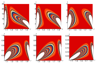
4.1 Estimation by quantum probes

Upon inspecting the functional dependence of the Bures metric on the quantities $t$, $\lambda$ and $\gamma$ in Eq. (9) one sees that $g_{B}(\gamma)$ is somehow a function of the quantity $\lambda t^{2\gamma}$ and thus maxima are expected, loosely speaking, for small $t$ and large $\lambda$ or viceversa. On the other hand, this scaling is not exact and thus a richer structure is expected. This is illustrated in Fig. 1, where we show contour plots of $g_{B}$ as a function of $\gamma$ and of the interaction time for different values of the coupling $\lambda$. As it is apparent from the plots, for any value of the coupling there are two maxima located in different regions (notice the different ranges for the interaction time). The global maximum moves from one region to the other depending on the values of the coupling (see below).

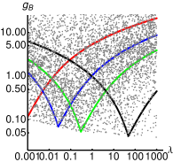
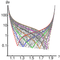
In Fig. 2 we show the results obtained from the numerical maximization of the Bures metric $g_{(}\gamma)$ over the interaction time. The upper left panel is a log-log-plot of the maximized Bures metric as a function of the coupling for randomly chosen values of $\gamma\in[1,2]$ and $\lambda\in[10^{-3},10^{3}]$ (gray points). We also report some curves at fixed values of $\gamma$, showing that for any value of the complementary Hurst parameter, except those close to the limiting values $\gamma=1$ and $\gamma=2$, a threshold value $\lambda_{\rm th}(\gamma)$ on the coupling, i.e. on the intensity of the noise, naturally emerges. The Bures metric is large, i.e. estimation may achieve high precision, in the weak and in the strong coupling limit, that is, when $\lambda\ll\lambda_{\rm th}(\gamma)$ or $\lambda\gg\lambda_{\rm th}(\gamma)$. On the other hand, for intermediate values of the coupling $\lambda\sim\lambda_{\rm th}(\gamma)$ the estimation of the fractal dimension is inherently inefficient. This behavior is further illustrated in the lower left panel, where we report the same random points as a function of $\gamma$, also showing curves at fixed values of the coupling. Values of $\gamma$ close to $\gamma=1$ or $\gamma=2$ may be precisely estimated for any value of the coupling whereas intermediate values needs a tuning of $\lambda$, in order to be placed in the corresponding weak (or strong) coupling limit. The threshold value $\lambda_{\rm th}(\gamma)$ increases with $\gamma$ and does not appear for $\gamma\simeq 1$ or $\gamma\simeq 2$. For those values high precision measurements are achievable only in the strong coupling limit (for $\gamma\simeq 1$, i.e. fractal dimension close to $\delta\simeq 2$) or the weak coupling limit ($\gamma\simeq 2$, i.e. negligible fractal dimension $\delta\simeq 1$).

Figure 2: Optimal estimation of the complementary Hurst parameter $\gamma$ by quantum probes. The upper left panel shows the maximized Bures metric as a function of the coupling for $5000$ randomly chosen values of $\gamma\in[1,2]$ (gray points) and $\lambda\in[10^{-3},10^{3}]$. The curves correspond to, from left to right, to $\gamma=1.2$ (red), $\gamma=1.4$ (blue) $\gamma=1.6$ (green), $\gamma=1.8$ (black). The upper right panel shows the optimal values $\tau_{B}$ of the interaction time, leading to the Bures metric of the left panel. The curves are for the same fixed values of $\gamma$ of the left panel. The lower left panel shows the the maximized Bures metric as a function of $\gamma$ for the same $5000$ randomly chosen values of $\gamma\in[1,2]$ (gray points) and $\lambda\in[10^{-3},10^{3}]$ of the upper panel. Here we report curves at fixed values of $\lambda=10^{k}$ with (from left to right) $k=-3,-2,-1,0,1,2,3$. The lower right panel shows the optimal values of the interaction time, leading to the Bures metric of the right panel.

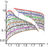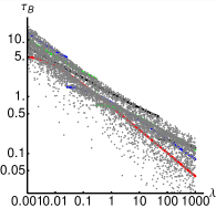
The right panels of Fig. 2 show the optimal values $\tau_{B}=\arg\max_{t}g_{B}(\gamma)$ of the interaction time, leading to the maximized values of the Bures metric reported in the left panels. The upper panel shows $\tau_{B}$ as function of the coupling whereas the lower one illustrates the behavior as a function of $\gamma$. Referring to the upper panel: $\tau_{B}$ exhibits a power-law decrease for small and large values of the coupling (notice the log-log scale the plots) whereas for intermediate values of $\lambda$ we observe a discontinuous behavior, which reflects the transition of the global maximum from from the peak at large $t$ and small $\lambda$ to the other one, located in the region of small $t$ and large $\lambda$.

The overall picture that we obtain from Fig. 2 is that quantum probes may be generally employed to obtain a reliable characterization of fractional Gaussian process, except when the coupling with the environment has intermediate values. These results may be understood intuitively as follows. The maxima obtained for small values of $\lambda$ correspond to quantum probes that are weakly coupled to the environment. In this case, decoherence is not much detrimental and for long interaction times the probe acquires information about the environmental parameters without being too much mixed, i.e. still storing this information in its quantum state. Viceversa, for a quantum probe strongly coupled to the environment, the information about the environmental parameters is quickly impinged onto the state of the quantum probe, such that it can effectively retrieved, upon performing measurements in the early stage of the evolution. In the intermediate situation, none of the two above effects take place: information is flowing from the environment to the probe too slowly compared to decoherence and no measurements can be effectively employed to extract it from the quantum state of the probe. The two regimes of weak and strong coupling are defined in terms of a threshold value of the coupling, which itself increases with the fractional dimension.

The above picture, however, does not apply when the fractal dimension of the trajectories is close to its limiting values, i.e. when the complementary Hurst parameter assumes values close to $\gamma=1$ or $\gamma=2$. In these two limiting cases no threshold on the coupling appears and $\gamma$ may be reliably estimated only in the weak coupling limit (for negligible fractal dimension) or in the strong coupling one (fractal dimension closer to its maximum value).

4.2 Discrimination by quantum probes

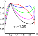
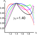
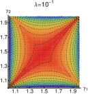
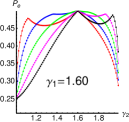
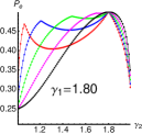
Let us now consider discrimination problems involving the complementary Hurst parameter. We assume to know in advance that only two possible values $\gamma_{1}$ and $\gamma_{2}$ are admissible and want to discriminate between them using the results of a measurement performed on the quantum probe. The Helstrom bound $P_{e}$ to the error probability in a single-shot discrimination is given in Eq. (10) and here we want to minimize $P_{e}$ over the interaction time. Results of the numerical minimization are shown in Fig. 2, where we report the minimized Helstrom bound as a function of $\gamma_{2}$ for different fixed values of $\gamma_{1}$, together with density plots of the same quantity as a function of the pair of values $(\gamma_{1},\gamma_{2})$ for different values of the coupling with the environment.

Figure 3: Helstrom bound to the discrimination of pairs of values of the complementary Hurst parameter by quantum probes. The four plots on the left panels show the Helstrom bound $P_{e}$ minimized over the interaction time as a function of $\gamma_{2}$ for different values of $\gamma_{1}$. In all the plots the different curves refer to different values of the coupling: $\lambda=10^{-2}$ (red), $\lambda=10^{-1}$ (blue), $\lambda=1$ (green), $\lambda=10$ (magenta), $\lambda=100$ (black). The two right panels show a density plot of the minimized Helstrom bound as a function of both the values $\gamma_{1}$ and $\gamma_{2}$ for two different values of the coupling: $\lambda=10^{-1}$ (top panel) and $\lambda=10$ (bottom panel). Blue regions correspond to smaller values of $P_{e}$.

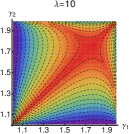The plots confirm the overall symmetry of the Helstrom bound $P_{e}(\gamma_{1},\gamma_{2})=P_{e}(\gamma_{2},\gamma_{1})$ at fixed $\lambda$. Another feature that emerges from Fig. 3 is that, say, the pairs $\gamma_{1}=1.2$ and $\gamma_{2}=1.4$ or $\gamma_{1}=1.4$ and $\gamma_{2}=1.6$ have different discriminability despite the fact that for both pairs we have $|\gamma_{1}-\gamma_{2}|=0.2$, i.e. the Helstrom bound is not uniform. The plots also confirm the overall picture obtained in discussing estimation problems: for each pair of values $(\gamma_{1},\gamma_{2})$, two regimes of strong or weak coupling may be individuated, where discrimination may be performed with reduced error probability, whereas for intermediate values of the coupling performances are degraded. The only exception regards values close to the limiting values $\gamma=1$ or $\gamma=2$, where no threshold appears.

We also notice that by increasing the coupling one enlarges the region in the $\gamma_{1}$-$\gamma_{2}$ plane where discrimination may be performed with reduce error probability. This is illustrated in the right panels of Fig. 3, where we show a density plot of the minimized Helstrom bound as a function of both the values $\gamma_{1}$ and $\gamma_{2}$ for two different values of the coupling: $\lambda=10^{-1}$ (top panel) and $\lambda=10$ (bottom panel)

Figure 4: Chernoff bound to the multiple-copy discrimination of pairs of values of the complementary Hurst parameter by quantum probes. In the left panel we report the maximized Chernoff bound as a function of the coupling with the environment for pair of values $(\gamma,\gamma+0.2)$ with $\gamma$ not too close to the limiting values $\gamma=1$ or $\gamma=2$. From left to right we have, $\gamma=1.2$ (blue squares), $\gamma=1.3$ (green triangles), $\gamma=1.4$ (red circles), $\gamma=1.5$ (magenta stars), $\gamma=1.6$ (gray squares), $\gamma=1.7$ (gray circles). In the right panel we show the same quantity for pair of values $(\gamma_{1},\gamma_{2})$ close to the boundaries $\gamma=1$ and $\gamma=2$. The increasing curves correspond to $\gamma_{1}=1.0,\gamma_{2}=1.1$ (blue circles), $\gamma_{1}=1.1,\gamma_{2}=1.2$ (blue stars), $\gamma_{1}=1.0,\gamma_{2}=1.2$ (blue triangles), whereas the decreasing ones are for $\gamma_{1}=1.8,\gamma_{2}=1.9$ (black circles), $\gamma_{1}=1.9,\gamma_{2}=2.0$ (black stars), $\gamma_{1}=1.8,\gamma_{2}=2.0$ (black triangles).

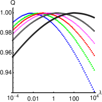
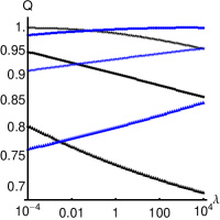
As mentioned in Section 3, the Helstrom bound to the single-shot error probability by quantum probes is bounded from below by the value $P_{e}\geq\frac{1}{4}$, making these kind discrimination schemes of little interest for applications. We are thus naturally led to consider multiple-copy discrimination. In Fig. 4 we report the results of the optimization of the Chernoff bound of Eq. (11) over the parameter $s$ and the interaction time. In the left panel we show the quantity $Q(\gamma_{1},\gamma_{2},\lambda)$, minimized over the interaction time, as a function of the coupling with the environment for different pairs of values $\gamma_{1}$ and $\gamma_{2}$ not too close to the limiting values $\gamma=1$ and $\gamma=2$. Also in this case, the plot also confirms that better performances are obtained in the regimes of weak and strong coupling, whereas for intermediate values no measurements are able to effectively extract information from the quantum probe. The threshold to define the two regimes increases with the value of the $\gamma$’s themselves. When the values of the Hurst parameter are approaching the limiting values $\gamma=1$ and $\gamma=2$ no threshold appears. In these two limiting cases discrimination may be reliably performed in the weak coupling limit (for negligible fractal dimension) or in the strong coupling one (fractal dimension closer to its maximum value). This behavior is illustrated in the right panel of Fig. 4, where we show the minimized $Q(\gamma_{1},\gamma_{2},\lambda)$ as a function of the coupling for pairs of values $\gamma_{1}$ and $\gamma_{2}$ close to $\gamma=1$ or $\gamma=2$.

For both, single- and multiple-copy discrimination, the behavior of the optimal interaction time is analogue to that observed in the discussion of estimation problem.

5 Conclusions

We have addressed estimation and discrimination problems involving the fractal dimension of fractional Brownian noise. Upon assuming that the noise induces a dephasing dynamics on a qubit, we have analyzed in details the performances of inferences strategies based on quantum limited measurements. In particular, in order to assess the performances of quantum probes, we have evaluated the Bures metric, the Helstrom bound and the Chernoff bound, and have optimized their values over the interaction time.

Our results show that quantum probes provide an effective mean to characterize fractional process in two complementary regimes: Either when the the system-environment coupling is weak, provided that a long interaction time is achievable, or when the coupling is strong and the quantum probe may be observed shortly after that the interaction has been switched on. The two regimes of weak and strong coupling are defined in terms of a threshold value of the coupling, which itself increases with the fractional dimension. Our results overall indicate that quantum probes may represent a valid alternative to characterize classical noise.

References

- [1] P. Sibani, J. H. Jensen, Stochastic dynamics of complex systems (World Scientific, New York, 2013).
- [2] D. J. Wilkinson, Nat. Rev. Gen. 10, 122 (2009).
- [3] D. Most, D. Keles, Eur. J. Op. Res. 207, 543 (2010).
- [4] P. E. Smouse, S. Focardi, P. R. Moorcroft, J. G. Kie, J. D. Forester, J. M. Morales, Phyl. Trans. Roy. Soc. B 365, 2201 (2010).
- [5] R. F. Fox, Phys. Lett. 48, 179 (1978).
- [6] B. B. Mandelbrot, J. W. Van Ness, SIAM Rev. 10, 432 (1968).
- [7] B. B. Mandelbrot, J. R. Wallis, Water Resour. Res. 4, 909 (1969).
- [8] M. S. Taqqu, Stat. Sci. 28, 131 (2013).
- [9] R. J. Barton, H. V. Poor, IEEE Trans. Inform. Th. 34, 943 (1988).
- [10] H. E. Hurst, Trans. Am. Soc. Civil. Eng. 116, 770 (1951).
- [11] P. Flandrin, IEE Trans. Inform. Th 35, 197 (1989).
- [12] R. B. Davies, D. S. Harte, Biometrika 74, 95 (1987).
- [13] H. D. Jeong, J. S. Lee, D. McNickle, and K. Pawlikowski, Simul. Model. Pract. Theory 15, 1173 (2007).
- [14] J. Barunik, L. Kristoufek, Physica A 389, 3844 (2010).
- [15] G. W. Wornell, A. V. Oppenheim, IEEE Trans. Signal Pro- cess. 40, 611 (1992).
- [16] L. Zunino, D. G. Peŕez, M. T. Martín, A. Plastino, M. Garavaglia, O. A. Rosso, Phys. Rev. E 75, 021115 (2007).
- [17] C. M. Kendziorski, J. B. Bassingthwaighte, P. J. Tonellato, Physica A 273, 439 (1999).
- [18] L. A. Salomon, J. C. Fort, J. Stat. Comp. Simul. 83, 542 (2013).
- [19] M. Magdziarz, J. K. S̀lezak, J. Wòjcik, J. Phys. A 46, 325003 (2013).
- [20] M. S. Taqqu, V. Teverovsky, W. Willinger, Fractals 3, 785 (1995).
- [21] Y. Liu, Y. Liu, K. Wang, T. Jiang, L. Yang, Phys. Rev. E 80, 066207 (2009).
- [22] D. Boyer, D. S. Dean, C Mejìa-Monasterio, G. Oshanin, Phys. Rev. E 87, 030103(R) (2013).
- [23] N. Makarava, S. Benmehdi, M. Holschneider, Phys. Rev. E 84, 021109 (2011).
- [24] J. Schmittbuhl, J.-P. Vilotte, S. Roux, Phys. Rev. E 51, 131 (1995).
- [25] A. Mehrabi, H. Rassamdana, M. Sahimi, Phys. Rev. E 56, 712 (1997).
- [26] C. Castelnovo, A. Podestà, P. Piseri, P. Milani, Phys Rev. E 65, 021601 (2002).
- [27] C. Benedetti, F. Buscemi, P. Bordone, M. G. A. Paris, Phys, Rev. A 89, 032114 (2014).
- [28] C. Benedetti, M. G. A. Paris, Int. J. Quantum Inf. 12, 1461004 (2014).
- [29] J. Řeháček, M. G. A. Paris (Eds) Quantum State Estimation, Lect. Not. Phys. 649 (Springer, Berlin, 2004)
- [30] I. Bengtsson, K. Zyczkowski, Geometry of Quantum States, (Cambridge University Press, 2006).
- [31] D. Bures, Trans. Am. Math. Soc. 135, 199 (1969).
- [32] A. Uhlmann, Rep. Math. Phys. 9, 273 (1976).
- [33] W. K. Wootters Phys. Rev. D 23, 357 (1981).
- [34] R. Josza, J. Mod. Opt. 41, 2314 (1994).
- [35] H.-J. Sommers, K. Zyczkowski, J. Phys. A 36, 10083 (2003).
- [36] S. Braunstein and C. Caves, Phys. Rev. Lett. 72, 3439 (1994).
- [37] S. Braunstein, C. Caves, and G. Milburn, Ann. Phys. 247, 135 (1996).
- [38] D. C. Brody, L. P. Hughston, Proc. Roy. Soc. Lond. A 454, 2445 (1998); A 455, 1683 (1999).
- [39] A. Sun-Ichi, H. Nagaoka, Methods of information geometry (AMS, 2000).
- [40] P. Zanardi, M. G. A. Paris, L. Campos-Venuti, Phys. Rev. A 78, 042105 (2008).
- [41] C. Invernizzi, M. Korbmann, L. Campos-Venuti, M. G. A. Paris, Phys. Rev. A 78, 042106 (2008).
- [42] M. G. A. Paris, Int. J. Quant. Inf. 7, 125 (2009).
- [43] M. Hotta, T. Karasawa, M. Ozawa, Phys. Rev. A 72, 052334 (2005).
- [44] A. Monras, M. G. A. Paris Phys. Rev. Lett. 98, 160401 (2007).
- [45] A. Fujiwara, Phys. Rev. A 63, 042304 (2001); A. Fujiwara, H. Imai, J. Phys. A 36, 8093 (2003).
- [46] Z. Ji, G. Wang, R. Duan, Y. Feng, M. Ying IEEE Trans. Inf. Theory, 54, 5172 (2008).
- [47] V. D’Auria, C. de Lisio A. Porzio, S. Solimeno, and M. G. A. Paris J. Phys. B 39, 1187 (2006).
- [48] M. Brunelli, S. Olivares, M. G. A. Paris, Phys. Rev. A 84, 032105 (2011); M. Brunelli, S. Olivares, M. Paternostro, M. G. A. Paris, Phys. Rev. A 86, 012125 (2012).
- [49] O. E. Barndorff-Nielsen, R. D. Gill, R. D, J. Phys. A 33, 4481 (2000).
- [50] A. Luati, Ann. Stat. 32, 1770 (2004).
- [51] C. W. Helstrom, Quantum Detection and Estimation Theory (Academic Press, New York 1976)
- [52] A. Chefles, Contemp. Phys. 41 401 (2000).
- [53] J. A. Bergou, U. Herzog, M. Hillery in [29], pp 417-465.
- [54] A. Chefles in [29], pp 467-511.
- [55] J. A. Bergou, J. Mod. Opt. 57, 160 (2010).
- [56] J. Calsamiglia, R. Munoz-Tapia, L. Masanes, A. Acín, E. Bagan, Phys. Rev. A 77, 032311 (2008).
- [57] K. M. R. Audenaert, J. Calsamiglia, R. Munoz-Tapia, E. Bagan, Ll. Masanes, A. Acin, F. Verstraete, Phys. Rev. Lett. 98, 160501 (2007).
- [58] M. Nussbaum, and A. Szkola, Ann. Stat. 37, 1040 (2009).
- [59] K. M. R. Audenaert, M. Nussbaum, A. Szkola, and F. Verstraete, Commun. Math. Phys. 279, 251 (2008).
- [60] S. Pirandola and S. Lloyd, Phys. Rev. A 78, 012331 (2008).
- [61] C. Invernizzi, M. G. A. Paris, S. Pirandola, Phys. Rev. A 84, 022334 (2011).