Abstract

Large whole-genome sequencing projects have provided access to much of the rare variation in human populations, which is highly informative about population structure and recent demography. Here, we show how the age of rare variants can be estimated from patterns of haplotype sharing and how these ages can be related to historical relationships between populations. We investigate the distribution of the age of variants occurring exactly twice ($f_{2}$ variants) in a worldwide sample sequenced by the 1000 Genomes Project, revealing enormous variation across populations. The median age of haplotypes carrying $f_{2}$ variants is 50 to 160 generations across populations within Europe or Asia, and 170 to 320 generations within Africa. Haplotypes shared between continents are much older with median ages for haplotypes shared between Europe and Asia ranging from 320 to 670 generations. The distribution of the ages of $f_{2}$ haplotypes is informative about their demography, revealing recent bottlenecks, ancient splits, and more modern connections between populations. We see the signature of selection in the observation that functional variants are significantly younger than nonfunctional variants of the same frequency. This approach is relatively insensitive to mutation rate and complements other nonparametric methods for demographic inference.

Author Summary

In this paper we describe a method for estimating the age of rare genetic variants. These ages are highly informative about the extent and dates of connections between populations. Variants in closely related populations generally arose more recently than variants of the same frequency in more diverged populations. Therefore, comparing the ages of variants shared across different populations allows us to infer the dates of demographic events like population splits and bottlenecks. We also see that rare functional variants shared within populations tend to have more recent origins than nonfunctional variants, which is likely to be the signature of natural selection.

Introduction

The recent availability of large numbers of fully sequenced human genomes has allowed, for the first time, detailed investigation of rare genetic variants. These are highly differentiated between populations [1, 2], may make an important contribution to genetic susceptibility to disease [3, 4, 5, 6, 7], and provide information about both demographic history, and fine-scale population structure [8, 9]. While patterns of rare variant sharing are informative in themselves, knowing the age of the variants allows us to observe changes in structure over time, and thus to infer the dates of demographic events.

Rare variants are typically more recent than common variants and in fact, the age of a variant can be estimated directly from its frequency [10, 11, 12]. However there are two problems with this approach. First, using only the frequency information means that we cannot distinguish differences between the ages of variants which are at the same frequency which, as we demonstrate here, can be both large and important. Second, in order to use this approach, we have to know the demographic history of the populations involved. In this article, we describe an alternative approach which uses the fact that the lengths of shared haplotypes around variants are informative about their ages [13, 14, 15].

Specifically, we estimate the time to the most recent common ancestor (TMRCA) for $f_{2}$ haplotypes, which are regions where two chromosomes are each other’s unique closest relative in a sample. To find these regions, we look for variants which occur exactly twice in the sample ($f_{2}$ variants, or doubletons). We then use nearby variation to estimate the extent of the $f_{2}$ haplotype and use the length of, and number of mutations on, this haplotype to infer its age, and therefore a lower bound for the age of the variant. Every $f_{2}$ variant identifies an $f_{2}$ haplotype, but we do not detect all $f_{2}$ haplotypes because not all of them carry mutations. This approach is fast, robust, and finds shared haplotypes directly from genotype data, which avoids the need for statistical phasing. We apply this method to the 1000 Genomes phase 1 dataset [16], to quantify the distribution of the ages of variants shared within and between populations, and between variants in different functional classes. We demonstrate dramatic differences between the ages of variants shared across different populations, and reveal the signatures of both demography and selective constraint.

Results

Figure 1: Algorithm and model for haplotypes. A: Algorithm for detecting $f_{2}$ haplotypes. For each $f_{2}$ variant in the sample (green), we scan left and right until we find inconsistent homozygote genotypes (red), record the physical and genetic length of this region (blue), and the number of singletons (purple). B: Model for haplotype age $t$. Consider the 4 chromosomes (grey) of the two individuals sharing an $f_{2}$ haplotype (blue). We model the total genetic length of the inferred haplotype, $L_{g}$, as the sum of the true genetic length $L_{g}^{*}$ and an error $\Delta_{g}$. Similarly, we model the number of singletons $S$ as the sum of the number on the shared chromosome ($S^{*}$) and the number on the unshared chromosomes, $\Delta_{S}$. We ignore the fact that we overestimate $L_{p}$ and therefore that some of the singletons might lie in the unshared part of the chromosome.

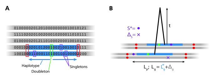
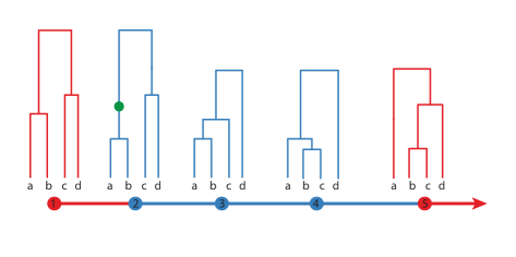
We first give a brief outline of our approach (Figures 1, S1, Methods). Given a sample of individual genotypes, we find all $f_{2}$ variants. That is, variants which have exactly two copies (in different individuals) in the sample. This tells us that, in the absence of repeat mutations and assuming that the $f_{2}$ variant is derived, those individuals must share an $f_{2}$ haplotype at that position. We then scan left and right along the genome, until we reach a point where the two individuals have inconsistent homozygote genotypes (0 and 2, Figure 1A).

Using both the genetic and physical lengths of the region, and the number of singletons, we compute an approximate likelihood for the age of the haplotype (Figure 1B). We use the data to estimate error terms to take into account the fact that the algorithm described above does not find the shared haplotypes precisely. Then, for each haplotype, we find the maximum likelihood estimate (MLE) of the age of each haplotype. We investigate the distribution of these MLEs for different classes of $f_{2}$ variants, for example those shared within or between specific populations.

Simulation results

Figure 2: Estimating $f_{2}$ age from simulated data. We simulated whole genomes for 100 individuals (200 chromosomes), with $N_{e}=14,000$, $\mu=1.2\times 10^{-8}$ and HapMap 2 recombination rates. A: Estimated age against true age. The grey dots are the MLEs for each detected haplotype. The blue line is a quantile-quantile (qq) plot for the MLEs (from the 1^st to 99^th percentile). B-D Power to detect $f_{2}$ haplotypes as a function of B: genetic length, C: physical length and D: haplotype age; in each case the darker line represents the power to detect $f_{2}$ haplotype with 100% power to detect $f_{2}$ variants, and the lighter line the power with 66% power to detect variants.

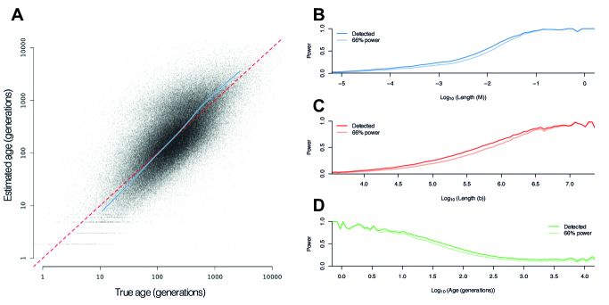
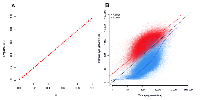
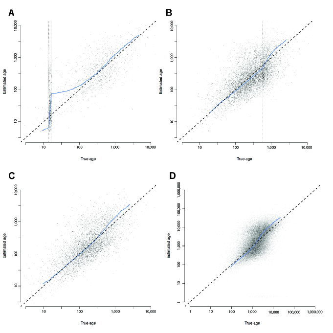
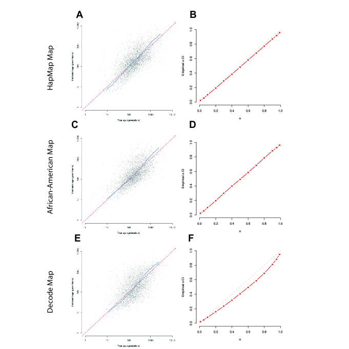
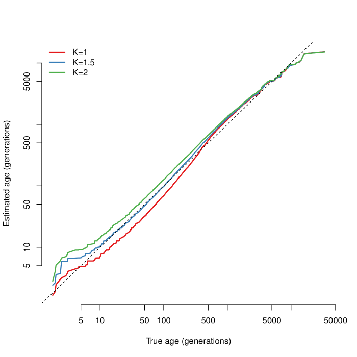
To test our approach, we ran whole genome simulations for a sample of 100 diploid individuals with MaCS[17], using the combined HapMap 2 recombination maps [18], and a mutation rate ($\mu$) of $1.2\times 10^{-8}$ per-base per-generation, assuming a constant effective population size ($N_{e}$) of 14,000; chosen to reflect parameters relevant to human genetic variation. We investigated both our power to detect the $f_{2}$ haplotypes and how accurately we could estimate the distribution of $f_{2}$ ages (Figure 2). We detected around 26% of all $f_{2}$ haplotypes. Unsurprisingly, we have more power to detect very long haplotypes, but we detected many small haplotypes as well: 19% of our total had true genetic length less than than 0.1cM. Having imperfect power to detect $f_{2}$ variants does not have a large effect on our power to detect $f_{2}$ haplotypes since most haplotypes carry more than one $f_{2}$ variant. We have higher power for more recent haplotypes because they are longer but, at least for a population of constant size, this effect is cancelled to some extent for older haplotypes because the branches above them tend to be longer and therefore more likely to carry mutations.

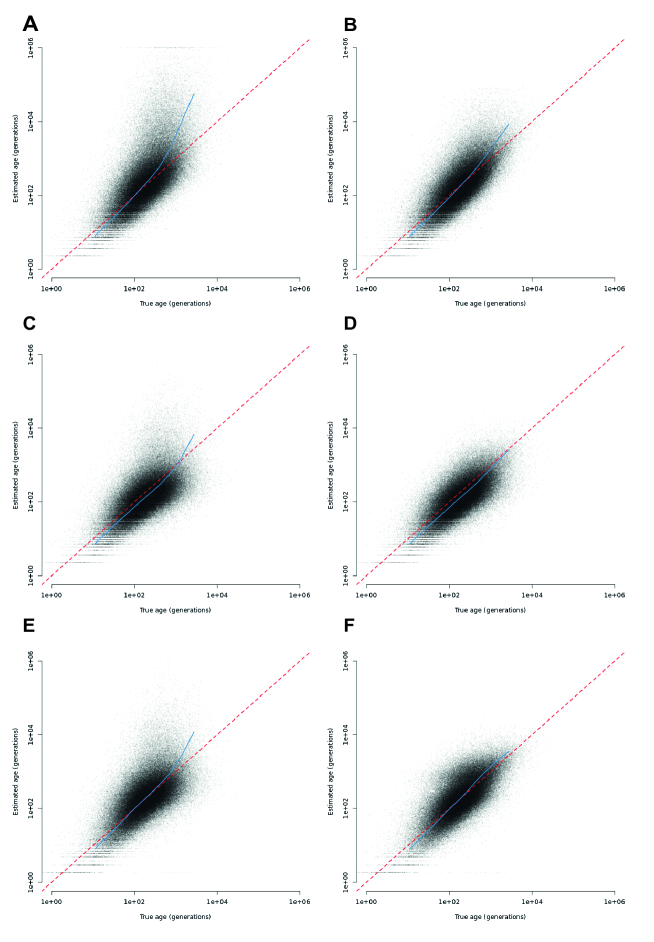
There is high uncertainly in the age of any individual haplotype (Figure 2A). However, we can compute well-calibrated confidence intervals (Figure S2). In this example, the median MLE of the age of the detected haplotypes is 179 generations and the true median is 192 generations. The median width of the 95% confidence interval is 730 generations. Information about the ages comes mainly from the genetic length, and the principal advantage of the singleton information is for very old haplotypes where the length-based estimator is otherwise biased (Figure S3).

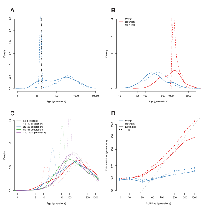
In addition, we ran simulations to check that the model was robust to more complicated demographic scenarios including splits, bottlenecks and expansions, as well as mis-specification of $N_{e}$ (Figure S4). We also investigated the effect that these scenarios had on the distribution of the ages of the $f_{2}$ haplotypes, demonstrating that we could detect the signatures of demographic events. For example, population bottlenecks lead to a high density of $f_{2}$ haplotypes during the bottleneck and, following a population split haplotypes shared between populations have median age roughly equal to the split time (Figure S5).

1000 Genomes data

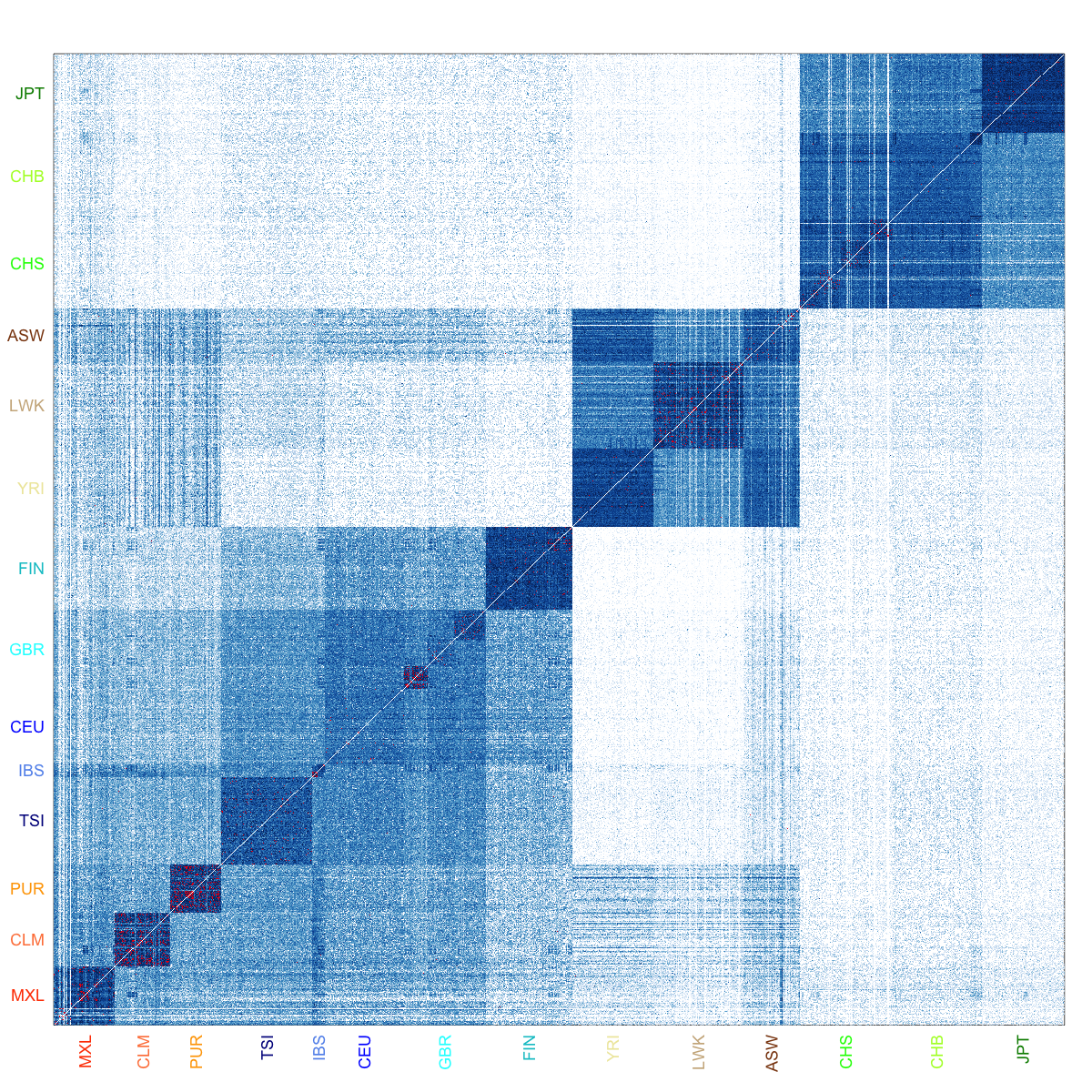
We applied our estimator to the phase 1 data release of the 1000 Genomes Project [16], which consists of whole-genome variant calls for 1,092 individuals drawn from 14 populations (Table 1). We used two of the 1000 Genomes callsets; one made from sequence data, and one made using a dense genotyping array. Restricting our analysis to the autosomes, we extracted $f_{2}$ variants from the sequence data callset, and then detected haplotype lengths around them (that is, the distances to incompatible homozygotes), using only the array data, to minimise the effect of genotyping errors. We then counted $f_{1}$ variants on these haplotypes from the sequence data callset. From 4,066,530 $f_{2}$ variants we detected 1,893,391 $f_{2}$ haplotypes, with median genetic and physical lengths of 0.7cM and 600kb respectively. The median number of singletons per haplotype was 3. Of the 1.9 million $f_{2}$ haplotypes, 0.7 million were shared within populations and 1.5 million were shared within continents. Sharing of $f_{2}$ variants largely reflects expected patterns of relatedness on a population level, and also reveals substructure in some populations, notably GBR (Figure S6).

Abbreviation	Sample size	Description
ASW	61	African Ancestry in SW USA
LWK	97	Luhya in Webuye, Kenya
YRI	88	Yoruba in Ibadan, Nigera
CLM	60	Colombians in Medellín, Colombia
MXL	66	Mexican Ancestry in Los Angeles, CA, USA
PUR	55	Puerto Ricans in Puerto Rico
CHB	97	Han Chinese in Beijing, China
CHS	100	Han Chinese South
JPT	89	Japanese in Tokyo, Japan
CEU	85	Utah residents with ancestry from northern and western Europe
FIN	93	Finnish in Finland
GBR	89	British from England and Scotland
IBS	14	Iberian Populations in Spain
TSI	98	Toscani in Italy

Table 1: Short descriptions of the 1000 Genomes populations.

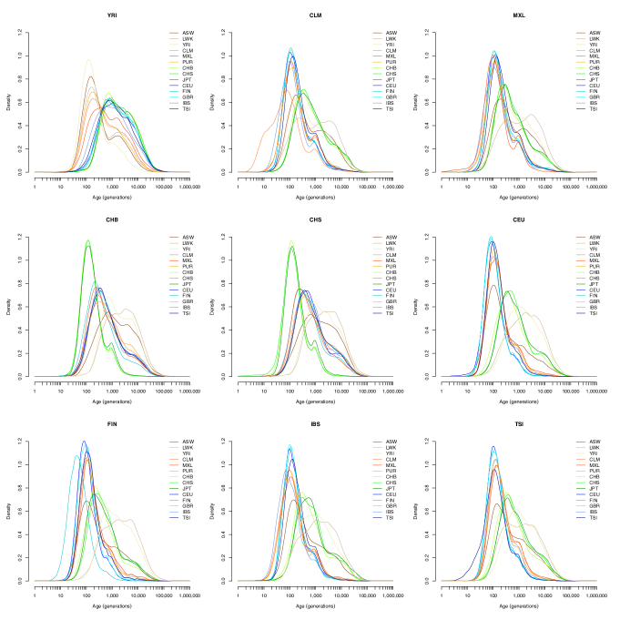
We used the combined recombination rate map from HapMap 2 to determine genetic lengths, and assumed a mutation rate of $0.4\times 10^{-8}$ per-base per-generation (reflecting a true mutation rate of $1.2\times 10^{-8}$ multiplied by a power of $\frac{1}{3}$ to detect singletons [19, 16]). We estimated $N_{e}=185,000$ (from the number of singletons in the dataset, Methods). We then computed MLEs for the ages of all the $f_{2}$ haplotypes shared between every pair of populations (Figures 3, S7, Tables S14-S18). We estimated that on most chromosomes the median overestimate in the haplotype lengths is 0.1-0.15cM (but more on chromosomes 1, 9 and 15), and that $\theta$ (estimated from singletons) was around $3.7\times 10^{-3}$ and $2.4\times 10^{-3}$ per-base for African and Non-African populations respectively (Table S19).

Figure 3: The estimated age distribution of $f_{2}$ haplotypes. A: The distribution of the MLE of the ages of haplotypes shared within each population. B-F: The distribution of the MLE of the ages of haplotypes shared between one population and all other populations, shown for each of GBR, JPT, LWK, ASW, and PUR. Populations are described in Table 1. Density estimates are computed in $\log_{10}$ space, using the base R “density” function with a Gaussian kernel.

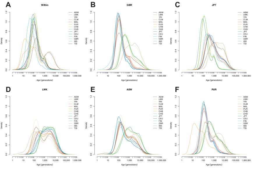
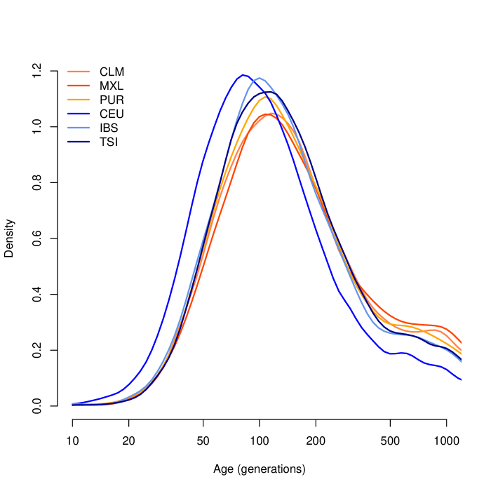
For haplotypes shared within populations (Figure 3A), the MLEs of haplotypes within most European and Asian populations are clustered around 100 generations ago. For example, the median age of GBR-GBR haplotypes is 90 generations. PUR and, to a lesser extent, CLM have many very recent haplotypes (peaking around 11 generations ago), consistent with a historical bottleneck in these populations 300-350 years ago. FIN haplotypes peak around 14 generations (400-450 years) ago. African populations have many recent haplotypes but also a much longer tail than the other populations, with ancestry apparently extending back for thousands of generations. For example the median age of LWK-LWK haplotypes is 320 generations, but the 95% quantile is 8,500 generations.

Between-population sharing is largely consistent with the historical relationships among populations (Figure 3B-D). Within continents, sharing within Asia or Europe has a median of 50-160 generations, depending on the populations, and sharing within Africa 170-340 generations. Sharing between continents is much older, with median Asian-European sharing 320-670 generations old, and Asian-African sharing rather older, with a median around 2,300 generations ago for LWK and 1,700 generations ago for YRI. The age of European-African sharing varies between populations, from 1,000 to 2,000 generations ago, but is more recent than Asian-African sharing, perhaps suggesting greater subsequent migration between these continents. We discuss these figures in the context of split times and migrations in the Discussion.

Admixed populations have age distributions that are combinations of the distributions of the admixing populations (Figure 3E-F). Even in these populations we can see signs of more subtle history. For example, GBR-CLM haplotypes have an age distribution which looks more like GBR-TSI or GBR-IBS than GBR-CEU, presumably representing the fact that the major contribution to European admixture in the Americas is from southern Europe (Figure S8).

Figure 4: The ages of haplotypes around $f_{2}$ variants with different functional annotations. Density is indicated by the width of the shape, and horizontal bars show the median. We show separately the densities for $f_{2}$ variants shared within a population (left, blue), and $f_{2}$ variants shared between populations (right, red). Numbers in brackets show the number of variants in each class. Bars show the pairwise differences in means, and $t$ test p-values for a difference in log means between groups.

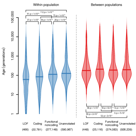
We also looked at the distribution of the ages of $f_{2}$ variants broken down by functional annotation (Figure 4, Methods). We found that for variants shared within a single population, loss-of-function (LOF) variants are younger than coding variants, which are younger than functional noncoding variants, and all annotated variants are younger than unannotated variants. The median ages of these variants are 58, 83, 112 and 125 generations for LOF, coding, functional noncoding and unannotated variants respectively. This is presumably because purifying selection against damaging mutations means that functional variants are less likely to become old (though positive selection for beneficial mutations would have the same effect). This effect has previously been both predicted and observed [20, 21]. However, it is not strictly true for variants shared between different populations and, in fact, the effect is partially reversed (median ages are 176, 205, 186 and 195 generations for LOF, coding, functional noncoding and unannotated variants). A likely explanation is that functional variants surviving long enough to be shared between populations are selectively neutral or recessive and thus unaffected by selection at low frequency. This suggests that studies looking for disease-causing rare variants should concentrate on variants private to a single population, since variants shared across populations are unlikely to have large phenotypic effects.

Robustness

This analysis requires us to estimate several parameters, and in this section, we investigate how robust it is to varying them.

The parameter $k$ is related to the probability of discovering $f_{2}$ haplotypes. We know that $1\leq k\leq 2$. $k=1$ implies that the probability that we discover a haplotype is independent of its length while $k=2$ implies that this probability increases linearly with length. We chose $k=1.5$ based on simulations, but it may be the case that this is not the optimal $k$ for real data. To test how much of an impact this might have, we re-ran the analysis of the 1000 Genomes data using $k=1$ and $k=2$. Larger values of $k$ increase our age estimates. For example, the median CEU-CHB age is 403, 481 and 560 generations using $k=1$, 1.5 and 2 respectively. Overall, setting $k=2$ increases the median age estimates by between 6 and 30%, depending on population, with more recent ages more sensitive to $k$.

The parameters $k_{e}$ and $\lambda_{e}$ are the shape and rate of the (gamma) distribution of the overestimate of haplotype lengths (Methods). We estimated these parameters separately from the array data for each chromosome (Table S19). We noticed that chromosomes 1, 5 and 9 had estimated parameters that implied a greater overestimate (larger $k_{e}$, smaller $\lambda_{e}$), presumably due to the density of markers on the array for those chromosomes. In addition, these chromosomes had older estimated haplotype ages, for example we estimated that the median age of $f_{2}$ haplotypes on chromosome 1 was 16% higher than the median age of haplotypes on chromosome 2, suggesting that our error model is not fully robust to variation in marker density.

Discussion

We described an approach to estimate the age of $f_{2}$ haplotypes, without making any prior assumptions about population structure or history. Though the age of any individual haplotype is uncertain, major features of the distribution of haplotype ages are detected, demonstrating qualitative differences between populations that are almost certainly due to past demographic events. The next important question is to what extent we can use these distributions as quantitative estimates of the ages of demographic events.

Figure 5: Comparison with MSMC, and the effect of estimating haplotypes with sequence data. A: The age distribution of $f_{2}$ haplotypes shared between CHB and CEU estimated with array, sequence and “clean” sequence (with indels and low complexity regions removed; Methods). Coloured dashed lines show the medians of each distribution. The grey stepped line shows relative cross-population coalescence rates estimated by MSMC (S. Schiffels, personal communication), and the grey dashed line shows the earliest point where this rate is less that 0.5. In both cases, we assume 30 years per generation and $\mu=1.25\times 10^{-8}$. B: As in A but for $f_{2}$ haplotypes shared between CHB and MXL, restricted to haplotypes where the MXL individual is inferred to be homozygous for Native American ancestry. C-D: Age distributions inferred using “clean” sequence data, comparable to Figure 3A-B (Note the extended x-axis).

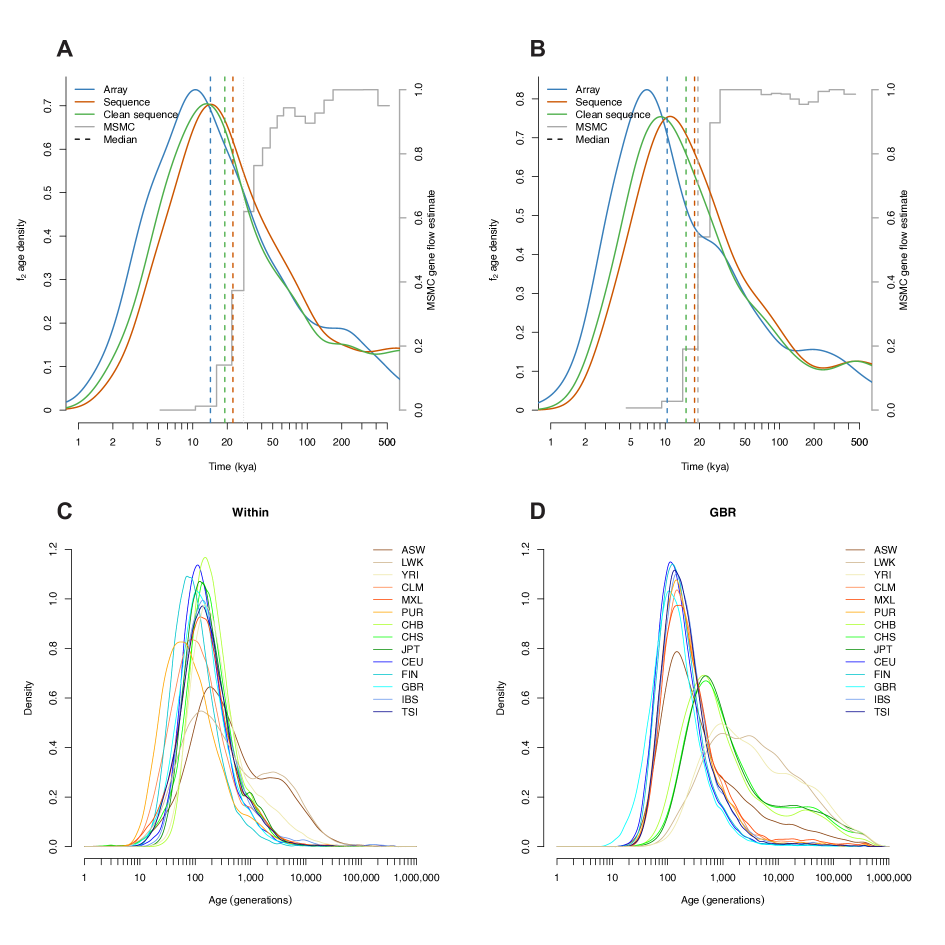
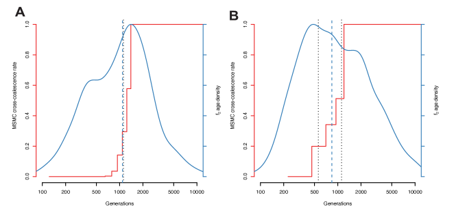
Consider the split between European and East Asian populations. Model based estimates of this split time have ranged from 14 to 40 thousand years ago (kya) [22, 23, 24]. Although, these are likely to be too low because they assumed a mutation rate, $\mu$, of $2-2.5\times 10^{-8}$ per-base per-generation, now thought to be an overestimate [19] and so a more reasonable range of estimates might be 22-80kya. The nonparametric PSMC approach[25] estimated a split time of around 22kya (if a lower mutation rate of $1.25\times 10^{-8}$ is used, 11kya with the higher rate), and a similar method, MSMC, estimates a split time of 20-40kya (S. Schiffels, personal communication; Figure 5A). Simulations suggest that, under a clean split model, the median of our estimated ages is close to or slightly below the split time, at least for recent splits (less than 1,000 generations; Figures S5 and S9). Comparing CEU to each of CHB, CHS and JPT, taking the median of our haplotype ages, and assuming a generation time of 30 years[26], would imply split times of 14, 17 and 18kya respectively. Other European populations give different estimates, but mostly between 15 and 20kya.

Similarly, when we looked at $f_{2}$ variants shared between East Asia and America (CHB-MXL, but restricting to regions homozygous for Native American ancestry in MXL; Methods), we found that the median age was around 10kya, substantially more recent than the split time estimated using MSMC (S. Schiffels, personal communication; Figure 5B). This seems low, given geological evidence that the Bering land bridge was submerged by 11-13kya, although a seasonal or maritime route likely remained open after that time [27, 28, 29].

Our dates are all around or below the low end of published estimates, even after we take into account the fact that the median might be lower than the split time (we estimate about 11% lower for a 500-generation old split; Figure S5D). There are several non-exclusive explanations for this observation. First, post-split gene flow could explain the discrepancy. As we have greater power to detect $f_{2}$ haplotypes if they are more recent, when the split is not clean many of the haplotypes we observe will derive from the post-split gene flow rather than from before the initial split (Figure S9B). In this scenario, we would be detecting the most recent haplotypes, and our dates would be closer to the most recent date of contact, rather than the initial split date.

An alternative explanation might be systematic errors in our estimates. As we described in the Results, the approach is sensitive to the estimated parameters $k$, $k_{e}$ and $\lambda_{e}$. At the extreme, increasing $k$ from 1.5 to its maximum value of 2 would increase the median age of CEU-CHB haplotypes from 14kya to 17kya. To investigate sensitivity to $k_{e}$ and $\lambda_{e}$, we repeated the analysis, but using sequence data rather than array data to find the length of the haplotypes (Figure 5). We note that when we estimated $k_{e}$ and $\lambda_{e}$ using sequence data they vary very little across chromosomes (Table S19). The ages estimated using sequence data were older than those estimated using array data (Median age of CEU-CHB haplotypes 23kya, Figure 5A-B). We might expect that sequence data, being more dense than array data, would find haplotypes more accurately. However we would also expect that genotype errors, more common in sequence than array data, would make all haplotypes look older, by incorrectly breaking haplotypes. Removing indels and low complexity regions (LCRs; Methods) thought to be enriched for genotyping errors from the sequence data reduced the difference (median CEU-CHB age of 19kya), suggesting that around half the increase in age is driven by errors. Further, the haplotype ages estimated from sequence data do not contain the very young (long) haplotypes within CLM, FIN and PUR, which we independently believe to be correct (Figure 5C), and also contain a long tail of extremely old haplotypes which seems unlikely (Figure 5D).

Another source of systematic errors could be the use of incorrect mutation or recombination rates. There is considerable uncertainty about the mutation rate in humans, but our approach is relatively insensitive to this, so if the true rate is higher than $\mu=1.25\times 10^{-8}$ per-base per-generation then mutational clock based methods which scale linearly with mutation rate will overestimate the ages of events, thus reducing the discrepancy.

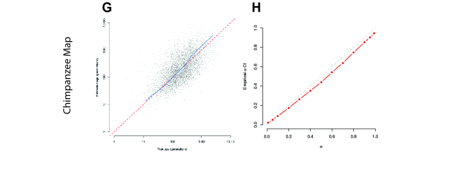
On the other hand, our approach might be sensitive to errors in the recombination map. We tested this by running simulations with a different genetic map to the HapMap map that we used to determine genetic length. We tested a population-based African American map[30], a map derived from an Icelandic pedigree [31] and a chimpanzee map from a small population[32], but none of these made a substantial difference to the results and we conclude that the length of the haplotypes we investigate is sufficiently large that they are robust to the uncertainty in the recombination map (Figure S11).

Finally, systematic errors might occur due to homoplasy (where the same mutation occurs independently on two different lineages). While this rate is expected to be low, it may be locally high in some parts of the genome, for example in CpG islands which have an order of magnitude higher mutation rate than the genomic background. If such false positives do occur, they would appear as very short haplotypes that we would infer to be very old, so they cannot explain our systematically lower ages. On the other hand, it is likely that some of the very old haplotypes we see are, in fact, due to repeat mutations and, in particular, this might explain some of the very old haplotypes discovered with sequence data.

However, while systematic biases in our estimates might explain some of the difference between our estimated ages and independent split time estimates, they cannot explain the observation that the age distributions vary greatly between different pairs of populations. This strongly suggests that there is variation in the extent of gene flow. For example, Asian-FIN sharing seems to be more recent than other Asian-European sharing, suggesting relatively recent contact between East Asian and Finnish populations, compared to other European populations. It seems likely that worldwide demographic history is sufficiently complicated that trying to estimate a single Asian-European (or African-Non African) split time is futile, and that a complex model of many splits, migrations and admixtures is required to explain the relationship between different populations.

Ultimately, we would like to be able to make explicit estimates of parameters like historical effective population size, and the dates of demographic events. Though the approach we describe here is limited in in this respect, there is a clear path to extend it to do so. We could first use a similar approach to estimate the age of variants at frequency three and higher. Then, treating the estimates of haplotype ages as estimates of coalescent times, we could use the empirical distribution of coalescent times to estimate population sizes and cross-population migration rates as a function of time. Another improvement would be to use information from the full likelihood surface for each haplotype, rather than just the point estimate of the age as we do here. Since, for large samples, we would have good estimates of recent coalescent rates, we expect that this approach would be very accurate at inferring recent history, making it a complementary approach to sequential Markovian coalescent based methods which are typically accurate in the ancient past, but less so for very recent history.

Methods

Definitions

Suppose we have a sample of size $N$ of genotypes from a single genetic region. Define an $f_{2}$ variant to be one which occurs exactly twice in the sample in different individuals. That is, either two individuals have genotype 1 and all the others have genotype 0, or two individuals have genotype 1 and the others have genotype 2. We assume that the minor allele is the derived allele. Under the neutral coalescent, for a sample of $2N$ chromosomes, an $f_{2}$ minor allele will be the derived allele with probability $\frac{2N-1}{2N+1}\approx 1$ for large $N$ so this is a reasonable assumption for large samples.

Define an $f_{2}$ haplotype shared between chromosomes $a$ and $b$ to be a region satisfying the following two conditions: 1) The time to the most recent common ancestor (TMRCA) of $a$ and $b$ does not change over the region. 2) At one or more sites in the region, $a$ and $b$ coalesce with each other before either of them coalesce with any other chromosome. In other words, they are unique genealogical nearest neighbours (Figure S1). We call the TMRCA of $a$ and $b$ the age of the haplotype. Additionally, we say that individuals $i$ and $j$ ($i\neq j$) share an $f_{2}$ haplotype if $a$ is one of $i$’s two chromosomes and $b$ is one of $j$’s two chromosomes.

The problem we solve is to find the $f_{2}$ haplotypes and then estimate their ages. Since each $f_{2}$ variant must lie in an $f_{2}$ haplotype, the variants provide a simple way of detecting the haplotypes. We use the algorithm described in the main text to find regions which should be larger than the $f_{2}$ haplotypes. The next problem is to determine the likelihood of the age. We describe our approximate likelihood below but first, as an example, we describe exact inference in the absence of confounding factors.

Exact case

Suppose we knew the exact genetic and physical lengths of an $f_{2}$ haplotype and the number of singletons it carries. Call these quantities $L_{g}^{*},L_{p}^{*}$ and $S^{*}$. Let the age of this haplotype be $t$ generations, or $\tau$ in coalescent time ($\tau=\frac{t}{2N_{e}}$). Then, for a randomly chosen $f_{2}$ haplotype (but not a haplotype at a randomly chosen position, discussed in the next section), $L_{g}^{*}$ has an exponential distribution with parameter $4N_{e}\tau$ and $S^{*}$ has a Poisson distribution with parameter $\theta L_{p}^{*}\tau$ where $\theta=4N_{e}\mu$ and $\mu$ is the per-base per-generation mutation rate. Therefore (ignoring terms that do not depend on $\tau$), the log-likelihood of $\tau$ given $L_{g}^{*},L_{p}^{*}$ and $S^{*}$ is

$$\ell\left(\tau;l_{g}^{*},l_{p}^{*},s^{*}\right)=\left(1+s^{*}\right)\log\left(\tau\right)-4N_{e}\tau l_{g}^{*}-\theta l_{p}^{*}\tau$$

and the maximum likelihood estimator of $t$ is therefore

$$\hat{t}=\frac{1+s^{*}}{2\left(l_{g}^{*}+\mu l_{p}^{*}\right)}.$$

Approximate likelihood for genetic length

There are two corrections to the likelihood for genetic length. The first relates to the ascertainment process of the haplotypes, and the second to the overestimate in the length due to the way we detect the endpoints.

The ascertainment problem is as follows. Suppose we pick a haplotype at random, then its length is exponentially distributed (i.e. gamma with shape parameter 1). However, if we pick a point on the sequence at random then the distribution of the length of the haplotype in which it falls is gamma distributed with shape parameter 2. This is an example of the “inspection paradox” and it is because in the second case, we are sampling haplotypes effectively weighted by their length. In our case, we detect haplotypes if they contain one or more $f_{2}$ variants. Therefore the probability that we find a haplotype is increasing with its physical length (because longer haplotypes are more likely to carry $f_{2}$ variants), but sub-linearly. The probability also increases with genetic length, but in a complex way that depends on the variation of recombination and mutation rate along the genome, the age of the haplotype and the demographic history of the population. For example, in a constant sized population, older haplotypes are likely to have longer branches above them, and therefore to have more $f_{2}$ variants, but in an expanding population the opposite may be true. Rather than trying to take all of these effects into account, we made the simplifying assumption that we could model the genetic length $L_{g}^{*}$ as a gamma distribution with shape parameter $k$ where $1<k<2$ and rate $4N_{e}\tau$. Simulations suggested that $k$ around 1.5 was optimal (Figure S11), and we used this value throughout.

The second correction involves the overestimate of genetic length. We tried to detect the ends of the haplotype by looking for inconsistent homozygote genotypes, but of course in practice, after the end of the $f_{2}$ haplotype, there will be some distance before reaching such a site. This (genetic) distance $\Delta_{g}$ is the amount by which we overestimate the length of the haplotype. We estimate the distribution of $\Delta_{g}$ for a given sample by sampling pairs of genotype vectors, then sampling sites at random and computing the sum of genetic distance to the first inconsistent homozygote site on either side. We then fit a gamma distribution with (shape, rate) parameters $(k_{e},\lambda_{e})$ to this distribution, for each chromosome. The likelihood of $\tau$ is given by the convolution density of $L_{g}^{*}$ and $\Delta_{g}$,

$$L(\tau;l_{g})=\int_{0}^{l_{g}}f_{\gamma}\left(x;\left(k,4N_{e}\tau\right)\right)f_{\gamma}\left(l_{g}-x;\left(k_{e},\lambda_{e}\right)\right)dx$$ (1)

where $f_{\gamma}\left(x;(\kappa,\lambda)\right)=\frac{1}{\Gamma(\kappa)}\lambda^{\kappa}x^{\kappa-1}e^{-\lambda x}$ is the density of a gamma distribution with (shape, rate) parameters $(\kappa,\lambda)$. This integral, and therefore the loglikelihood $\ell(\tau;l_{g})=\log\left[L(\tau;l_{g})\right]$ can be expressed in terms of the confluent hypergeometric function $\,{}_{1}F_{1}$ (ignoring terms that do not depend on $\tau$),

$$\ell(\tau;l_{g})=k\log(\tau)+\log\left[\,{}_{1}F_{1}\left(k,k+k_{e},l_{g}\left(\lambda_{e}-4N_{e}\tau\right)\right)\right].$$ (2)

Where, recall, we assume $k=1.5$. Note that if we replace $2N_{e}\tau$ with $t$, and drop constant terms, then we get an expression for the likelihood of $t$ that does not depend on $N_{e}$, so our estimate of time in generations does not depend on $N_{e}$.

$$\ell(t;l_{g})=k\log(t)+\log\left[\,{}_{1}F_{1}\left(k,k+k_{e},l_{g}\left(\lambda_{e}-2t\right)\right)\right].$$ (3)

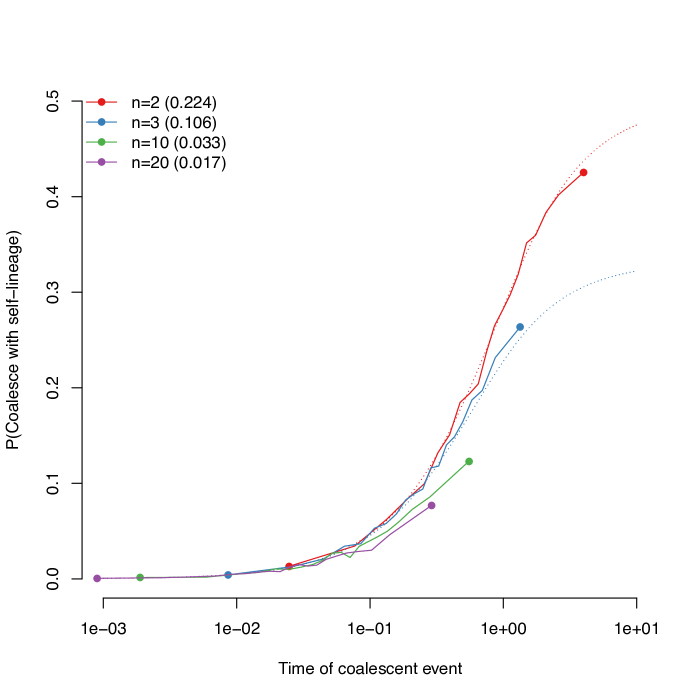
Finally, note that the rate at which recombination events occur on the branch connecting the two shared haplotypes is $4N_{e}\tau$. We assume that the first such event marks the end of the haplotype. However, there is a non-zero probability that a recombination event occurring on this branch does not change the MRCA of $a$ and $b$. Simulations suggest that for large numbers of chromosomes, this probability is extremely small (Figure S12) and so we assume it is 0. In practice, for small samples, this might be a non-negligible effect.

Approximate likelihood for singleton count

Recall that the physical length of the shared haplotype is $L_{p}$ bases. We assume that we can find this exactly. Then assuming a constant mutation rate $\mu$ per base per generation, the sum of the number of singletons on the shared haplotypes, $S^{*}$ has a Poisson distribution with parameter $\theta L_{p}\tau$, where $\theta=4N_{e}\mu$.

Now consider the distribution of singletons on the unshared haplotypes. To approximate this distribution, we make the following three assumptions: 1) There is no recombination on the unshared haplotypes over the region. 2) No other lineage coalesces with the shared haplotype before it is broken. 3) The distribution of the time to first coalescence of the unshared haplotypes is exponential with parameter $N$ (Recall that $N$ is the number of sampled individuals). In fact the true distribution is a mixture of exponentials but the approximation at least matches the correct mean, $\frac{1}{N}$ [33]. The variance is too small because of the first assumption, however.

Consider one of the unshared haplotypes. Conditional on the time ($\tau_{1}$) at which it first coalesces with any other haplotype, the number of singleton mutations it carries is Poisson with parameter $\theta L_{p}\tau_{1}$ and so, using the assumptions above, the unconditional distribution is geometric (on $0,1\dots$) with parameter $\frac{1}{1+\frac{\theta L_{p}}{2N}}$. Therefore the distribution of the number of mutations on both unshared haplotypes, $\Delta_{S}$, is the sum of two geometric distributions which is negative binomial with parameters $\left(2,\frac{\theta L_{p}}{\theta L_{p}+2N}\right)$. The density of the total number of singletons, $S$ is the convolution of these two densities

$$L(\tau;l_{p},s)=\sum_{x=0}^{s}f_{Po}\left(x;\theta l_{p}\tau\right)f_{NB}\left(s-x;\left(2,\frac{\theta l_{p}}{\theta l_{p}+2N}\right)\right)$$ (4)

where $f_{Po}\left(x;\lambda\right)=\frac{\lambda^{x}e^{-\lambda}}{x!}$ is the density of a Poisson distribution with parameter $\lambda$ and $f_{NB}\left(x;\left(n,p\right)\right)=\binom{x+n-1}{x}(1-p)^{n}p^{x}$ is the density of a negative binomial distribution with parameters $(n,p)$. As with the genetic length, we can write this in terms of $t$, the haplotype age in generations,

$$L(t;l_{p},s)=\sum_{x=0}^{s}f_{Po}\left(x;2\mu l_{p}t\right)f_{NB}\left(s-x;\left(2,\frac{\theta l_{p}}{\theta l_{p}+2N}\right)\right)$$ (5)

In practice we assume $\mu$ is known and estimate $\theta$ separately for each individual, for each chromosome, by counting the number of singletons, multiplying by the number of chromosomes in the sample, and dividing by the chromosome length. Then for each pair, we use use the average of these values in Equation 5. A more accurate approach would be to compute the likelihood as a double convolution over the distribution of both haplotypes with different values for $\theta$. An extension would be to estimate $\theta$ separately for different regions of the genome.

Approximate full likelihood

We can now write the approximate log-likelihood for $t$ as the sum of Equation 3 and the log of Equation 5, assuming that the recombination process is independent of the mutational process,

$$\ell(t;l_{g},l_{p},s)=\ell(t;l_{g})+\log\left[L(t;l_{p},s)\right].$$ (6)

We maximise it numerically with respect to $t$ in order to find the maximum likelihood estimate (MLE). It is possible for this likelihood to be bimodal, in which case we might find a local but not global optimum. However, this seems to be rare.

1000 Genomes Data

The 1000 Genomes data was obtained from ftp://ftp.1000genomes.ebi.ac.uk/vol1/ftp/. The phase 1 release sequence data is in phase1/analysis_results/integrated_call_sets, and the array data is in phase1/analysis_results/supporting/omni_haplotypes. In order to generate the “clean” sequence data, we removed any sites that fell in the list of low complexity regions found in technical/working/20140224_low_complexity_regions/hs37d5-LCRs.txt. Functional annotations are in phase1/analysis_results/functional_annotation. Detailed explanations of the annotations can be found there, but briefly the classifications are as follows:

• Loss-of-function: Includes premature stop codons, and essential splice site disruptions.

• Coding: Variants in coding regions.

• Functional noncoding: Including variants in noncoding RNAs, promoters, enhancers and transcription factor binding sites.

• Unannotated: Any variant not included in any of the above categories.

We included haplotypes in more than one of these categories if they contained multiple variants.

Code

All the code we used to run simulations and analyse the 1000 Genomes data is available from www.github.com/mathii/f2.

Supplementary information

Figure S 1: Example of an $f_{2}$ haplotype. Recombination events are shown as a series of marginal trees, as we move left to right along a sequence, so the tree above point $x$ is constant between $x$ and $x+1$. In the blue region, $a$ and $b$ share an $f_{2}$ haplotype. At sites 2 and 3, $a$ and $b$ are unique nearest neighbours. A mutation at site 2 (green), will be detected as an $f_{2}$ variant. At site 4, they are no longer unique nearest neighbours, but the TMRCA is unchanged. At site 5, the TMRCA has changed and the haplotype breaks. In the other direction, at site 1 the haplotype breaks because the TMRCA of $a$ and $b$ changes, even though they are still unique nearest neighbours. We count this as breaking the haplotype, even though we cannot detect this event.

Figure S 2: Confidence intervals. A: Coverage of approximate confidence intervals. We performed simulations as described in Figure 2, but only for chromosome 20. We computed approximate $\alpha$-confidence intervals using the $\chi^{2}$ approximation to the distribution of the log-likelihood. This figure shows the proportion of true haplotype ages that lie inside their approximate confidence intervals. B: Confidence intervals for the simulations in Figure 2. For each haplotype, we plot its true age against the upper and lower end of the two-tailed 95% confidence interval.

Figure S 3: The effect of different terms of the likelihood. This shows plots comparable to Figure 2, based on whole-genome simulations of 100 individuals. Grey dots show the estimated age of each $f_{2}$ haplotype against the true age. The blue line is a qq plot of the distribution of the MLEs (from 1% to 99% quantiles) Each subfigure shows the result of using different information. A, C and E use just the genetic length and B, D and F use both the genetic length and the number of singletons. A and B show the results if the true values are used in the likelihood. C and D show the corresponding results when the observed length is used without accounting for the overestimate, E and F (the same as Figure 2A) show the full likelihood, including the correction to $L_{g}$.

Figure S 4: The effect of demography on the accuracy of inference. These plots were generated with the same parameters as Figure 2 ($N_{e}=14,000$, $\mu=1.2\times 10^{-8}$), but show only chromosome 20. Grey dots show the estimated age of each detected $f_{2}$ haplotype against the true age (in generations). The blue line is a qq plot of the distribution of the MLEs (from 1% to 99% quantiles). We simulated different demographic scenarios. A: A bottleneck which reduces the population by 99% between 14 and 17 generations in the past (dotted lines). B: A population of size 14,000 which split into two isolated populations, each of size 14,000, 560 generations ago (dotted line). C: A population growing exponentially by about 0.02% per generation, to a present size of 140,000. D: A population where $N_{e}$ is actually 140,000 but we ran inference assuming it to be 14,000.

Figure S 5: The effect of demography on inferred age distributions. Solid lines show the density estimate of the distribution of the MLEs of the ages of detected $f_{2}$ haplotypes under different demographic scenarios. Dashed lines show the true distributions. Parameters as in Figure 2. A: A recent bottleneck. Dotted lines show the time of the bottleneck (population size reduced by 99% for 3 generations).B: Population split 1120 generations ago with no subsequent migration. The dotted line shows the time of the population split. The blue line shows the estimated age of $f_{2}$ variants shared within a population and the red line the estimated age of $f_{2}$ variants shared between populations. The red dotted line shows the median of this distribution and the black dotted line shows the split time. C: Distributions for different bottlenecks. As in A but now reducing the population size by 90% for 5 generations and using the recombination map from chromosome 10 instead of 20. D: Median within and between population ages, both estimated (solid line) and true (dashed line), for different split times. As in B, but again using the chromosome 10 recombination map

Figure S 6: $f_{2}$ variant sharing across 1000 Genomes individuals. Colours from white to blue to red show the number of $f_{2}$ variants shared between each pair of individuals, normalised by the total in each row. Individuals are ordered by populations, but only by sample name within each population.

Figure S 7: 1000 Genomes $f_{2}$ haplotype MLE age distributions. For the nine populations not included in Figure 3. Each of these subfigures shows the distribution of ages of haplotypes shared between one population and each of the others.

Figure S 8: GBR-American sharing. The density of the ages of $f_{2}$ haplotypes shared between GBR (UK) and each of CEU (NW European), CLM (Columbian), IBS (Spanish), MXL (Mexican), PUR (Puerto Rican) and TSI (Tuscan). See Table 1 for more complete descriptions of the populations.

Figure S 9: The effect of post-split migration. Comparison of the distribution of the age of $f_{2}$ variants shared between populations (blue) and the gene flow estimated by MSMC with 4 haplotypes (red). $N_{e}=14,000$, $\mu=1.2\times 10^{-8}$, using the chromosome 20 recombination map. In each case, the blue dashed line shows the median of the $f_{2}$ age distribution. a: A scenario where the two populations split 1120 generations ago (black dashed line). b: A scenario where two populations split 1120 generations ago, but there is migration at a rate of 1% per year for 560 generations (black dashed lines at 560 and 1120 generations). Note that in b, the peak of the $f_{2}$ age density is shifted to the left relative to a, indicating that many of the $f_{2}$ variants shared between populations derive from post-split migration rather than predating the split.

Figure S 10: This figure is continued on the next page.

Figure S 11: The effect of errors in the recombination map. We simulated haplotypes with a different recombination map to the one used to determine genetic length. The left column shows true versus estimated ages for detected haplotypes, and a qq plot of the MLEs, as in Figure 2A in the main text. The right column shows the coverage of the asymptotic confidence intervals as in Figure 2A. Each row shows the results of simulations using a different map (references in main text), but in every case the HapMap combined map was used to determine the genetic length of the detected haplotypes: A,B: Simulated using the HapMap map. C,D: Simulated using a map derived from African Americans. E,F: Simulated using a map derived from an Icelandic pedigree. G,H: Simulated using a map derived from chimpanzees, rescaled to have the same total length as the human map. In each case, we simulated Chromosome 20 for 100 individuals with $\mu=1.2\times 10^{-8}$ per-base per-generation and $N_{e}=14,000$.

Figure S 12: Effect of varying $k$. This figure shows the effect on the density estimate of varying $k$, the shape parameter of the gamma distribution used to model the genetic length of the haplotypes. This shows qq plots generated from simulations as in Figure 2, but for chromosome 20 only, for $k=1$, 1.5 and 2.

Figure S 13: Probability that recombinations do not change the TMRCA. We used simulations to estimate the probability that the first recombination on the branch between two haplotypes which are nearest neighbours does not change their TMRCA. For varying sample sizes $n$, we simulated sequences with recombination using the SMC’ algorithm. We find pairs of nearest neighbours, then count along the sequence until the first recombination on the branch connecting them. The plot shows the probability that this recombination does not change the TMRCA ($\tau$) of those two samples, as a function of $\tau$. Solid circles show 5% and 95% quantiles of the distribution of coalescence times. The dashed lines show the theoretical lower bounds on this probability; $\frac{1}{n}\left(1-\frac{1}{nt}\left(1-e^{-nt}\right)\right)$, exact for $n=2$, which is achieved if there are no coalescences on the tree except the one between the two nearest neighbour lineages. The numbers in brackets in the legend show the probability that a recombination does not change the TMRCA, averaged over all events. Note that as $n$ increases, for fixed $\tau$, the probability of not changing the TMRCA decreases, but in addition the distribution of $\tau$ becomes smaller which also decreases the probability of not changing the TMRCA.

	ASW	LWK	YRI	CLM	MXL	PUR	CHB	CHS	JPT	CEU	FIN	GBR	IBS	TSI
ASW	32,995	68,828	96,214	11,175	10,027	11,486	3,700	3,730	3,244	7,794	4,944	8,412	1,595	8,748
LWK	68,828	135,521	88,596	11,871	9,591	12,288	4,946	5,044	4,675	4,330	3,085	4,541	1,403	8,905
YRI	96,214	88,596	101,317	11,216	8,044	12,253	3,421	3,514	3,256	2,578	1,932	2,838	795	4,375
CLM	11,175	11,871	11,216	22,080	17,268	12,516	2,888	2,594	2,581	13,483	8,007	15,120	4,992	19,860
MXL	10,027	9,591	8,044	17,268	30,772	12,397	4,359	4,091	3,981	12,559	7,685	13,560	4,196	18,973
PUR	11,486	12,288	12,253	12,516	12,397	15,732	2,062	1,891	1,807	12,742	7,065	13,674	3,777	19,367
CHB	3,700	4,946	3,421	2,888	4,359	2,062	60,480	113,761	65,147	2,886	3,401	3,003	664	4,667
CHS	3,730	5,044	3,514	2,594	4,091	1,891	113,761	69,260	52,616	2,509	2,559	2,812	579	3,960
JPT	3,244	4,675	3,256	2,581	3,981	1,807	65,147	52,616	109,214	2,446	2,965	2,744	581	3,672
CEU	7,794	4,330	2,578	13,483	12,559	12,742	2,886	2,509	2,446	21,517	24,260	41,902	5,089	36,671
FIN	4,944	3,085	1,932	8,007	7,685	7,065	3,401	2,559	2,965	24,260	51,084	24,475	3,084	19,161
GBR	8,412	4,541	2,838	15,120	13,560	13,674	3,003	2,812	2,744	41,902	24,475	27,314	6,344	35,757
IBS	1,595	1,403	795	4,992	4,196	3,777	664	579	581	5,089	3,084	6,344	1,502	6,931
TSI	8,748	8,905	4,375	19,860	18,973	19,367	4,667	3,960	3,672	36,671	19,161	35,757	6,931	43,068

Table S 14: 1000 Genomes $f_{2}$ haplotype total counts. Counts of $f_{2}$ haplotypes shared between each pair of populations.

	ASW	LWK	YRI	CLM	MXL	PUR	CHB	CHS	JPT	CEU	FIN	GBR	IBS	TSI
ASW	18.03	11.63	17.92	3.05	2.49	3.42	0.63	0.61	0.60	1.50	0.87	1.55	1.87	1.46
LWK	11.63	29.11	10.38	2.04	1.50	2.30	0.53	0.52	0.54	0.53	0.34	0.53	1.03	0.94
YRI	17.92	10.38	26.47	2.12	1.38	2.53	0.40	0.40	0.42	0.34	0.24	0.36	0.65	0.51
CLM	3.05	2.04	2.12	12.47	4.36	3.79	0.50	0.43	0.48	2.64	1.43	2.83	5.94	3.38
MXL	2.49	1.50	1.38	4.36	14.35	3.42	0.68	0.62	0.68	2.24	1.25	2.31	4.54	2.93
PUR	3.42	2.30	2.53	3.79	3.42	10.59	0.39	0.34	0.37	2.73	1.38	2.79	4.91	3.59
CHB	0.63	0.53	0.40	0.50	0.68	0.39	12.99	11.73	7.55	0.35	0.38	0.35	0.49	0.49
CHS	0.61	0.52	0.40	0.43	0.62	0.34	11.73	13.99	5.91	0.30	0.28	0.32	0.41	0.40
JPT	0.60	0.54	0.42	0.48	0.68	0.37	7.55	5.91	27.89	0.32	0.36	0.35	0.47	0.42
CEU	1.50	0.53	0.34	2.64	2.24	2.73	0.35	0.30	0.32	6.03	3.07	5.54	4.28	4.40
FIN	0.87	0.34	0.24	1.43	1.25	1.38	0.38	0.28	0.36	3.07	11.94	2.96	2.37	2.10
GBR	1.55	0.53	0.36	2.83	2.31	2.79	0.35	0.32	0.35	5.54	2.96	6.97	5.09	4.10
IBS	1.87	1.03	0.65	5.94	4.54	4.91	0.49	0.41	0.47	4.28	2.37	5.09	16.51	5.05
TSI	1.46	0.94	0.51	3.38	2.93	3.59	0.49	0.40	0.42	4.40	2.10	4.10	5.05	9.06

Table S 15: 1000 Genomes $f_{2}$ haplotype mean counts. Mean number of $f_{2}$ haplotypes shared between each pair of individuals, for each pair of populations.

	ASW	LWK	YRI	CLM	MXL	PUR	CHB	CHS	JPT	CEU	FIN	GBR	IBS	TSI
ASW	337	527	247	385	406	371	1,306	1,272	1,503	184	232	190	311	358
LWK	527	317	308	897	1,178	781	2,374	2,295	2,227	1,795	2,013	1,833	1,377	1,224
YRI	247	308	168	421	651	351	1,640	1,710	1,649	1,449	1,453	1,394	996	1,209
CLM	385	897	421	70	148	152	536	555	606	143	144	143	117	179
MXL	406	1,178	651	148	115	156	402	432	441	148	159	150	131	191
PUR	371	781	351	152	156	38	583	629	620	135	135	137	126	166
CHB	1,306	2,374	1,640	536	402	583	137	140	149	481	321	499	496	483
CHS	1,272	2,295	1,710	555	432	629	140	134	158	581	421	600	612	606
JPT	1,503	2,227	1,649	606	441	620	149	158	110	615	380	621	650	667
CEU	184	1,795	1,449	143	148	135	481	581	615	98	99	100	129	130
FIN	232	2,013	1,453	144	159	135	321	421	380	99	48	106	131	132
GBR	190	1,833	1,394	143	150	137	499	600	621	100	106	90	128	133
IBS	311	1,377	996	117	131	126	496	612	650	129	131	128	97	158
TSI	358	1,224	1,209	179	191	166	483	606	667	130	132	133	158	120

Table S 16: 1000 Genomes $f_{2}$ haplotype medians. Median estimated age (in generations) of the MLE of the $f_{2}$ haplotypes shared between each pair of populations, using array data to estimate the haplotypes.

	ASW	LWK	YRI	CLM	MXL	PUR	CHB	CHS	JPT	CEU	FIN	GBR	IBS	TSI
ASW	43	56	54	57	58	57	127	114	154	36	38	37	53	55
LWK	56	21	55	65	83	62	266	267	264	146	183	165	116	116
YRI	54	55	44	63	75	59	255	238	241	173	197	182	115	147
CLM	57	65	63	7	35	34	94	92	95	41	41	42	27	49
MXL	58	83	75	35	25	37	78	83	82	43	44	43	29	51
PUR	57	62	59	34	37	6	89	98	95	41	40	42	29	47
CHB	127	266	255	94	78	89	44	44	47	78	64	86	90	87
CHS	114	267	238	92	83	98	44	34	49	101	79	106	105	104
JPT	154	264	241	95	82	95	47	49	32	106	74	109	111	111
CEU	36	146	173	41	43	41	78	101	106	29	33	32	41	41
FIN	38	183	197	41	44	40	64	79	74	33	13	35	40	41
GBR	37	165	182	42	43	42	86	106	109	32	35	15	40	42
IBS	53	116	115	27	29	29	90	105	111	41	40	40	24	45
TSI	55	116	147	49	51	47	87	104	111	41	41	42	45	18

Table S 17: 1000 Genomes $f_{2}$ haplotype 5% quantiles. 5% quantile of estimated age (in generations) of the MLE of the $f_{2}$ haplotypes shared between each pair of populations, using array data to estimate the haplotypes.

	ASW	LWK	YRI	CLM	MXL	PUR	CHB	CHS	JPT	CEU	FIN	GBR	IBS	TSI
ASW	7,962	10,586	5,468	8,978	9,744	8,199	18,082	17,514	18,524	8,507	10,064	7,509	10,143	10,604
LWK	10,586	8,542	7,413	13,162	14,561	11,548	21,792	21,506	19,650	18,776	21,241	19,008	17,184	16,092
YRI	5,468	7,413	2,871	8,094	10,538	6,802	17,223	17,887	17,090	16,361	17,094	15,967	14,148	16,412
CLM	8,978	13,162	8,094	1,238	2,064	2,268	11,347	12,275	12,946	1,587	1,906	1,606	1,480	2,005
MXL	9,744	14,561	10,538	2,064	1,291	2,369	9,987	9,292	10,130	1,909	2,466	1,988	1,761	2,221
PUR	8,199	11,548	6,802	2,268	2,369	1,039	11,186	13,069	11,695	1,417	1,574	1,397	1,506	1,704
CHB	18,082	21,792	17,223	11,347	9,987	11,186	1,084	1,127	1,286	10,739	7,552	11,562	12,424	10,677
CHS	17,514	21,506	17,887	12,275	9,292	13,069	1,127	1,108	1,369	12,347	9,867	12,524	12,862	12,118
JPT	18,524	19,650	17,090	12,946	10,130	11,695	1,286	1,369	1,204	12,723	8,429	13,806	16,332	12,959
CEU	8,507	18,776	16,361	1,587	1,909	1,417	10,739	12,347	12,723	765	741	780	1,177	1,117
FIN	10,064	21,241	17,094	1,906	2,466	1,574	7,552	9,867	8,429	741	296	757	1,089	1,188
GBR	7,509	19,008	15,967	1,606	1,988	1,397	11,562	12,524	13,806	780	757	709	1,174	1,158
IBS	10,143	17,184	14,148	1,480	1,761	1,506	12,424	12,862	16,332	1,177	1,089	1,174	1,154	1,397
TSI	10,604	16,092	16,412	2,005	2,221	1,704	10,677	12,118	12,959	1,117	1,188	1,158	1,397	1,137

Table S 18: 1000 Genomes $f_{2}$ haplotype 95% quantiles. 95% quantile of estimated age (in generations) of the MLE of the$f_{2}$ haplotypes shared between each pair of populations, using array data to estimate the haplotypes.

Chr	$k^{Array}_{e}$	$\lambda^{Array}_{e}$	$k^{Seq}_{e}$	$\lambda^{Seq}_{e}$	$\theta_{Afr}$	$\theta_{N.Afr}$
1	0.413	60	0.386	222	3.47	2.18
2	0.539	186	0.377	260	3.79	2.45
3	0.580	234	0.389	278	3.88	2.44
4	0.576	215	0.382	276	3.94	2.40
5	0.564	213	0.374	263	3.80	2.44
6	0.570	228	0.386	282	3.76	2.39
7	0.588	222	0.380	278	3.62	2.38
8	0.533	195	0.378	275	4.24	2.57
9	0.468	78	0.406	264	3.48	2.03
10	0.557	195	0.393	253	3.90	2.41
11	0.561	236	0.369	273	3.88	2.52
12	0.585	215	0.398	259	3.74	2.35
13	0.528	178	0.389	250	3.35	2.00
14	0.507	156	0.390	273	3.23	2.03
15	0.350	46	0.373	203	3.20	1.96
16	0.619	213	0.430	308	3.74	2.41
17	0.506	138	0.388	235	3.66	2.31
18	0.616	222	0.416	277	3.94	2.44
19	0.652	218	0.431	291	3.41	2.28
20	0.617	226	0.407	252	3.73	2.46
21	0.611	162	0.428	191	2.90	1.82
22	0.526	138	0.421	258	2.32	1.60

Table S 19: Estimated error parameters for 1000 Genomes data. We show error parameters $k_{e}$ and $\lambda_{e}$ for each chromosome estimated with both array and sequence data, and $\theta$ ($\times 10^{-3}$) estimated by counting singletons, for each chromosome, showing the median value for non-African (N.Afr) and African (Afr) populations separately. Note that there is substantial variation in error parameters between chromosomes using array but not sequence data, suggesting that this is due to variations in the density of markers on the array, when we use array data to estimate the haplotypes.

References

- [1] Bustamante CD, Burchard EG, De la Vega FM (2011) Genomics for the world. Nature 475: 163–165.
- [2] Nelson MR, Wegmann D, Ehm MG, Kessner D, St Jean P, et al. (2012) An abundance of rare functional variants in 202 drug target genes sequenced in 14,002 people. Science 337: 100–104.
- [3] Nejentsev S, Walker N, Riches D, Egholm M, Todd JA (2009) Rare variants of IFIH1, a gene implicated in antiviral responses, protect against type 1 diabetes. Science 324: 387–389.
- [4] Johansen CT, Wang J, Lanktree MB, Cao H, McIntyre AD, et al. (2010) Excess of rare variants in genes identified by genome-wide association study of hypertriglyceridemia. Nature Genetics 42: 684–687.
- [5] McClellan J, King MC (2010) Genetic Heterogeneity in Human Disease. Cell 141: 210–217.
- [6] Rivas MA, Beaudoin M, Gardet A, Stevens C, Sharma Y, et al. (2011) Deep resequencing of GWAS loci identifies independent rare variants associated with inflammatory bowel disease. Nature Genetics 43: 1066–1073.
- [7] Beaudoin M, Goyette P, Boucher G, Lo KS, Rivas MA, et al. (2013) Deep resequencing of GWAS loci identifies rare variants in CARD9, IL23R and RNF186 that are associated with ulcerative colitis. PLoS Genetics 9: e1003723.
- [8] Gravel S, Henn BM, Gutenkunst RN (2011) Demographic history and rare allele sharing among human populations. Proceedings of the National Academy of Sciences 108: 11983–11988.
- [9] Mathieson I, McVean G (2012) Differential confounding of rare and common variants in spatially structured populations. Nature Genetics 44: 243–246.
- [10] Kimura M, Ohta T (1973) The age of a neutral mutant persisting in a finite population. Genetics 75: 199–212.
- [11] Griffiths RC, Tavaré S (1998) The age of a mutation in a general coalescent tree. Communications in Statistics Stochastic Models 14: 273–295.
- [12] Fu W, O’Connor TD, Jun G, Kang HM, Abecasis G, et al. (2013) Analysis of 6,515 exomes reveals the recent origin of most human protein-coding variants. Nature 493: 216–220.
- [13] Palamara PF, Lencz T, Darvasi A, Pe’er I (2012) Length distributions of identity by descent reveal fine-scale demographic history. American Journal of Human Genetics 91: 809–822.
- [14] Ralph P, Coop G (2013) The geography of recent genetic ancestry across Europe. PLoS Biology 11: e1001555.
- [15] Harris K, Nielsen R (2013) Inferring demographic history from a spectrum of shared haplotype lengths. PLoS Genetics 9: e1003521.
- [16] 1000 Genomes Project Consortium (2012) An integrated map of genetic variation from 1,092 human genomes. Nature 491: 56–65.
- [17] Chen GK, Marjoram P, Wall JD (2009) Fast and flexible simulation of DNA sequence data. Genome Research 19: 136–142.
- [18] International HapMap Consortium (2007) A second generation human haplotype map of over 3.1 million SNPs. Nature 449: 851–861.
- [19] Scally A, Durbin R (2012) Revising the human mutation rate: implications for understanding human evolution. Nature Reviews Genetics 13: 745–753.
- [20] Maruyama T (1974) The age of a rare mutant gene in a large population. American Journal of Human Genetics 26: 669–673.
- [21] Kiezun A, Pulit SL, Francioli LC, van Dijk F, Swertz M, et al. (2013) Deleterious alleles in the human genome are on average younger than neutral alleles of the same frequency. PLoS Genetics 9: e1003301.
- [22] Keinan A, Mullikin JC, Patterson N, Reich D (2007) Measurement of the human allele frequency spectrum demonstrates greater genetic drift in East Asians than in Europeans. Nature Genetics 39: 1251–1255.
- [23] Gutenkunst RN, Hernandez RD, Williamson SH (2009) Inferring the joint demographic history of multiple populations from multidimensional SNP frequency data. PLoS Genetics 5: e1000695.
- [24] Gronau I, Hubisz MJ, Gulko B, Danko CG, Siepel A (2011) Bayesian inference of ancient human demography from individual genome sequences. Nature Genetics 43: 1031–1034.
- [25] Li H, Durbin R (2011) Inference of human population history from individual whole-genome sequences. Nature 475: 493–496.
- [26] Fenner JN (2005) Cross-cultural estimation of the human generation interval for use in genetics-based population divergence studies. American Journal of Physical Anthropology 128: 415–423.
- [27] Brigham-Grette J, Anderson PM, Lozhkin AV, Glushkova OV (2004) Paleoenvironmental conditions in western Beringia before and during the Last Glacial Maximum. In: Madsen DB, editor, Entering America. Northeast Asia and Beringia Before the Last Glacial Maximum., University of Utah Press. pp. 29–61.
- [28] Keigwin LD, Donnelly JP, Cook MS, Driscoll NW, Brigham-Grette J (2006) Rapid sea-level rise and Holocene climate in the Chukchi Sea. Geology 34: 861–864.
- [29] Meltzer DJ (2009) First Peoples in a New World. Colonizing Ice Age America. Univ of California Press.
- [30] Hinch AG, Tandon A, Patterson N, Song Y, Rohland N, et al. (2011) The landscape of recombination in African Americans. Nature 476: 170–175.
- [31] Kong A, Gudbjartsson DF, Sainz J, Jonsdottir GM (2002) A high-resolution recombination map of the human genome. Nature 31: 241–247.
- [32] Auton A, Fledel-Alon A, Pfeifer S, Venn O, Ségurel L, et al. (2012) A fine-scale chimpanzee genetic map from population sequencing. Science 336: 193–198.
- [33] Blum MGB, François O (2005) Minimal clade size and external branch length under the neutral coalescent. Advances in Applied Probability 37: 647–662.