Local CP-violation and electric charge separation by magnetic fields from lattice QCD
Abstract
We study local CP-violation on the lattice by measuring the local correlation between the topological charge density and the electric dipole moment of quarks, induced by a constant external magnetic field. This correlator is found to increase linearly with the external field, with the coefficient of proportionality depending only weakly on temperature. Results are obtained on lattices with various spacings, and are extrapolated to the continuum limit after the renormalization of the observables is carried out. This renormalization utilizes the gradient flow for the quark and gluon fields. Our findings suggest that the strength of local CP-violation in QCD with physical quark masses is about an order of magnitude smaller than a model prediction based on nearly massless quarks in domains of constant gluon backgrounds with topological charge. We also show numerical evidence that the observed local CP-violation correlates with spatially extended electric dipole structures in the QCD vacuum.
Keywords:
chiral magnetic effect, finite temperature, lattice QCD, external field1 Introduction
Quantum Chromodynamics (QCD) is the theory of the strong interactions. At low temperatures QCD is confining, implying that the elementary particles of the theory - quarks and gluons - only exist as components of bound states (hadrons). The asymptotic freedom property of QCD ensures that at high temperatures the interaction between quarks and gluons weakens, and a transition to the quark-gluon plasma (QGP) phase occurs, where the dominant degrees of freedom are no longer colorless bound states but colored objects. According to lattice simulations, this transition is no real phase transition but an analytic crossover Aoki:2006we and takes place at around , see e.g. Refs. Aoki:2006br ; Borsanyi:2010bp .
The high-temperature QGP phase is routinely produced in contemporary high energy heavy-ion collisions, for example at the Relativistic Heavy Ion Collider (RHIC), where temperatures exceeding can be reached Adare:2009qk . Besides extreme temperatures, another interesting feature of such a heavy-ion collision is the presence of strong magnetic fields generated by the spectator particles in non-central events. This magnetic field is perpendicular to the reaction plane and may reach values up to GeV for RHIC and GeV for the Large Hadron Collider (LHC) Skokov:2009qp , depending on the beam energy and centrality. Even though the generated magnetic field has a very short lifetime, of the order of fm/, this magnetic ‘pulse’ coincides with the formation of the quark-gluon plasma and thus may play an important role in the description of the collision. Strong magnetic fields also represent an important concept for cosmology Vachaspati:1991nm and for the description of dense neutron stars called magnetars Duncan:1992hi . Therefore, a clear theoretical understanding of the response of QCD matter to external magnetic fields is desirable.
An important characteristic of the QCD vacuum is its transformation property under parity (P) and charge conjugation (C). In the absence of a -parameter, the theory prohibits violation of both the P- and CP-symmetries. Indeed, experimental bounds – mostly coming from measurements of the electric dipole moment of the neutron – on the degree of this violation turn out to be extremely tiny. Nevertheless, CP-violation could still be realized in the local sense, through fluctuations of CP-odd observables. One manifestation of this in the QGP phase created in heavy-ion collisions might be through the presence of domains with a non-trivial topological structure of the gluon fields (see, e.g., Ref. Kharzeev:1998kz ). Such a nonzero topology is indicated by the non-vanishing value of the topological charge (defined below) within that particular domain. Since the magnetic field is odd under CP transformation, it is natural to expect that it can be used to effectively probe the CP-odd domains of the quark-gluon plasma and, thus, the CP-violating fluctuations in the QCD vacuum.
A possible realization of the coupling between the strong magnetic field and the non-trivial topological structure of the QGP is the so-called chiral magnetic effect (CME) Kharzeev:2007jp ; Fukushima:2008xe . For close to massless quarks, helicity is an approximately conserved quantity, and in strong magnetic fields the quark spins tend to align themselves either parallel (for positive charges) or antiparallel (for negative charges) to the external field. Therefore, right-handed, positively charged quarks and left handed, negatively charged quarks will tend to have their momenta parallel to the direction of the magnetic field. In a domain of the quark-gluon plasma with nonzero topological charge density, there is an imbalance between the number of left- and right-handed quarks, due to the Atiyah-Singer index theorem. As a consequence, a net current of quarks can be produced (anti)parallel to the external magnetic field, or, equivalently, the domain in question will be electrically polarized in the direction of the magnetic field. An alternative formulation of the effect is in terms of a chiral chemical potential Fukushima:2008xe , which couples to the anomalous axial current and creates a chiral imbalance by preferring right-handed over left-handed quarks.
The effects of the electric polarization of the plasma domains may persist at later stages of the collision. After hadronization takes place, this can result in a preferential emission of charged particles above and below the reaction plane Kharzeev:2004ey ; Voloshin:2004vk . Indications for such a charge asymmetry were observed in the STAR experiment at RHIC Voloshin:2008jx ; Abelev:2009ac and in the ALICE experiment at the LHC Selyuzhenkov:2011xq . However, to access observables related to the CME, certain parity-even experimental backgrounds have to be taken into account, which complicates the interpretation of the observed data. Thus, the exact meaning of these results is still debated, see, e.g., Refs. Wang:2009kd ; Muller:2010jd ; Voronyuk:2011jd ; Bzdak:2012ia . For recent reviews on the subject see, e.g., Refs. Fukushima:2012vr ; Kharzeev:2013ffa .
The CME and topology-induced CP-violation have been studied in various approaches, ranging from effective theory/model calculations to Euclidean lattice simulations. The former include among others settings like the Nambu-Jona-Lasinio model with an additional coupling to the Polyakov loop (PNJL model) Fukushima:2010fe , the holographic approach Yee:2009vw ; Rebhan:2009vc , hydrodynamics (see, e.g., Refs. Zakharov:2012vv ; Kalaydzhyan:2012ut ) or using a chiral effective action Khaidukov:2013sja . On the lattice, the CME was first studied by measuring current- and chirality fluctuations in quenched Buividovich:2009wi and quenched gauge theory Braguta:2010ej . Surprisingly, around the transition temperature, the fluctuations of the current parallel to the magnetic field were found to decrease with growing in the small magnetic field region Buividovich:2009wi , a result which still lacks a qualitative understanding. Another approach to investigate the CME on the lattice is using the chiral chemical potential, see Refs. Yamamoto:2011gk ; Buividovich:2013hza . Finally, the interplay between magnetic fields and topology was also studied by discretizing a continuum instanton configuration, and measuring the electric polarization in the presence of the magnetic field Abramczyk:2009gb , see the illustration in the left panel of Fig. 1.

In the present paper, we pursue a different approach and measure the extent to which the topological charge and the electric polarization of the quarks correlate locally, when exposed to external magnetic fields. Instead of having to consider classical instanton configurations, this approach enables us to use real QCD gauge backgrounds and to consider the local fluctuations of the topological charge on them, see the right panel of Fig. 1. Moreover, while there is no need to introduce any anomalous current or chemical potential, the method still gives a handle on relating the topological and the electromagnetic properties of the QCD vacuum in a Lorentz invariant manner. This approach is similar to that of Ref. Buividovich:2009my , where chirality–electric polarization correlators were measured in quenched gauge theory to detect the induced electric dipole moment of valence quarks. However, in our case the quarks and the external magnetic field are introduced dynamically, which allows us to observe spatially extended electric dipole structures in the QCD vacuum.
We indeed find that in local domains with nonzero topological charge density, an electric dipole moment is induced parallel to the external field. The strength of this effect is determined for various magnetic fields and temperatures around for several different lattice spacings. A scheme for defining the continuum limit of the results, utilizing the gradient flow Luscher:2010iy of the fields, is also introduced and used to perform the continuum extrapolation. Finally we compare the lattice results to a model calculation that employs nearly massless quarks and constant (anti)selfdual gluon backgrounds – a setting in which the problem can be treated analytically Basar:2011by . This comparison reveals that the numerical result found for full non-perturbative QCD with physical quark masses is by an order of magnitude smaller than the model prediction.
2 Formulation
In our setup, we consider the local correlation of the quark electric dipole moment with the topological charge density,
| (1) |
where is the field strength at the point , and tr denotes the trace in color space. The space-time integral of gives the total topological charge . In order to define the local electric dipole moment operator, let us consider the spin polarization of the quark of flavor (represented by the field ),
| (2) |
where are the Euclidean Dirac matrices. In the presence of a constant Abelian external field , the spin polarization develops a nonzero expectation value Ioffe:1983ju ,
| (3) |
where is the charge of the quark of flavor , and the factor of proportionality is conventionally written as the product of the quark condensate and the magnetic susceptibility. Note that the expectation value in Eq. (3) involves an integral over space-time and a normalization by the four-volume, to exploit translational invariance.
The component of Eq. (3) is induced by an external magnetic field , whereas the component by an external (Euclidean) electric field . Accordingly, the polarizations correspond to a magnetic and an electric dipole moment of the quark, respectively111Note that this definition of the electric dipole moment is normalized with respect to the quark charge . To compare to, e.g. Ref. Kharzeev:2007jp , one should consider . . The electric dipole moment is a parity-odd quantity, just as the topological charge density of Eq. (1); their product is therefore parity-even, and can have a nonzero expectation value in the presence of the external magnetic field. We consider this product locally and write it, similarly to Eq. (3), as
| (4) |
where we factored out the magnitude of the topological fluctuations to define the correlator of the two quantities. A similar combination was studied in Ref. Buividovich:2009my . Since we use the square root of the expectation value of for the normalization. In this way, similarly to Eq. (3), we obtain an observable with mass dimension 3, and introduce the proportionality factor . We emphasize that we consider the product of the two densities on the left hand side locally, in order to see the local correlation of topology and the polarization (this local product contains contact terms which need to be removed by an adequate renormalization prescription, see Sec. 3 below). Eq. (4) expresses the fact that there is a local correlation between the topological charge density of the non-Abelian vacuum and the induced electric dipole moment, and that this correlation is proportional to the external magnetic field222 This mechanism may be compared to the Witten-effect, through which a magnetic monopole develops an electric charge via interacting with a (CP-odd) axion field Witten:1979ey ..
Consider now the ratio of Eq. (4) and the component of Eq. (3). Here the external field cancels to leading order, giving directly the ratio ,
| (5) |
which has dimension zero, and is particularly suited for the lattice determination. Note that in this ratio all multiplicative renormalization factors cancel.
3 Observables and renormalization
We calculate the expectation values appearing in Eq. (5) on the lattice with an external magnetic field in the positive direction, . The lattice geometry is , and the lattice spacing is denoted by , such that the spatial volume of the system is given by and the temperature by . We consider the three lightest quark flavors and , for which the charges are (here is the elementary charge). We derive our observables from the QCD partition function, which, in the staggered discretization of the fermionic action reads
| (6) |
where is the inverse gauge coupling, the gauge action and the fermion matrix, for which we apply two steps of stout smearing on the gluonic links . The quark masses are tuned along the line of constant physics (LCP) as , ensuring that the isospin averaged zero-temperature hadron masses equal their experimental values Borsanyi:2010cj (for the present action the most precise LCP can be read off from Fig. 1 of Ref. Borsanyi:2013bia ). Further details of the action and the simulation setup can be found in Refs. Aoki:2005vt ; Borsanyi:2010cj ; Bali:2011qj . Since the external field couples directly only to quarks, enters only through the fermion determinants. Note that the dependence on is always of the form of the renormalization group invariant combination .
For the gauge action , we use the tree-level improved Symanzik action, which contains the product of links along closed loops of size (the plaquettes ) and of size . The topological charge (1) at the space-time point can be calculated via the field strength , which can be discretized as the sum of the antihermitian part of the four plaquettes touching the site ,
| (7) |
and the product in the four plaquettes starts at point and advances counter-clockwise. To suppress the noise originating from short-range fluctuations, the links used in Eq. (7) are the twice stout smeared links that we also use in fermionic observables. We find that this choice for the definition of – and, thus, of – reduces the noise in the correlation between and the electric dipole moment, necessary for the coefficient of Eq. (5). Note that the continuum limit of is unaffected by this choice. Let us add here that it is customary to use improved definitions of (see, e.g., Ref. DeGrand:1997gu ) or much more extensive smearing of the gluonic links in order to obtain an integer value for the total topological charge . Here we do not aim to determine the total charge, or its susceptibility, but concentrate on local fluctuations in and its correlation with fluctuations of the electric dipole moment, for which we carefully checked that our setup is appropriate.
The expectation value of the spin polarization with respect to the partition function (6) reads
| (8) |
where the trace (in color and coordinate space) is determined using noisy estimators , such that the polarization at point is (color indices are suppressed here)
| (9) |
with no summation over . Here, is the number of estimators, which we set, depending on the ensemble, in the range . Furthermore, stands for the staggered representation of the tensor operator, see Ref. Bali:2012jv for the implementation we use.
Using the expressions (1), (7), (8) and (9), the expectation values appearing in the ratio of Eq. (5) are determined. The so obtained is yet to be renormalized, since both its numerator and denominator contain divergent terms. The magnetic dipole moment, for example, contains a logarithmic additive divergence, which may be eliminated using the operator , see Ref. Bali:2012jv . The square of is also subject to renormalization, as it contains the contact term, see, e.g., Ref. Bruckmann:2011ve . Similarly, one expects the numerator to contain terms that are infinite in the continuum limit. These divergences are related to the fact that two densities are multiplied at the same space-time point. To remove these unphysical contributions, we use the gradient flow Luscher:2010iy for the fields contained in and in . The gradient flow was shown to eliminate additive divergences in fermionic observables like the condensate or the pseudoscalar correlator Luscher:2013cpa . Likewise, we find that evolving the fields up to a fixed physical flow time – or, equivalently, applying a nonzero smearing range – renormalizes the observable and, at the same time, suppresses noise considerably. Our implementation of the gradient flow is detailed in App. A.
Finally, the operator is also subject to multiplicative renormalization by the tensor renormalization constant , which was calculated in perturbation theory for the present action in Ref. Bali:2012jv . However, this factor cancels in the ratio . Altogether, is ultraviolet finite, if the continuum limit is approached along a fixed nonzero smearing range . On the lattice, this corresponds to taking the limit at a fixed temperature and tuning the smearing range in lattice units as . We repeat the continuum extrapolation for several ranges and subsequently extrapolate the results to .
Let us point out that in the present study smearing is applied in two different contexts. First, stout link smearing is employed in the fermionic action in order to suppress lattice discretization errors and, thus, to improve the convergence towards the continuum limit. Second, the fields in certain observables are evolved according to the gradient flow, which is equivalent to performing infinitesimal smearing steps. The latter reduces unphysical ultraviolet contributions in some observables, allowing for a clean definition of the continuum limit.
4 Results
We first analyze the response of to the external magnetic field. Together with the results for , this is plotted for the down quark in the upper left panel of Fig. 2. The ratio of the two expectation values is expected to be independent of the magnetic field, up to corrections of ), in accordance with Lorentz invariance. Within the range of the applied magnetic fields, these corrections are found to be small, and thus the ratio is to a good approximation constant, see the lower left panel of Fig. 2. In order to determine the leading order -dependence of the ratio, in the following we fit the data either to a constant, or consider corrections of . Our strategy for the determination of the systematic error of the result will be discussed below.
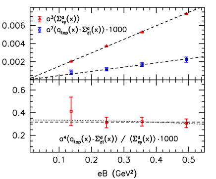
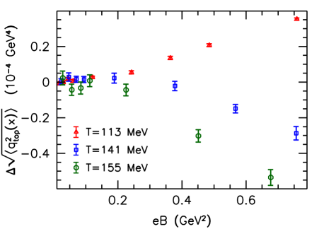
The next step to obtain the coefficient of Eq. (5) is to measure the local fluctuations333Note that measures the extent of local fluctuations, in contrast to the topological susceptibility , which quantifies the global fluctuations. in . We find that depends quadratically on (again in accordance with Lorentz invariance), however, with a coefficient that changes sign as the temperature is increased across the transition temperature . This behavior is reminiscent of that of the chiral condensate Bali:2011qj ; Bali:2012zg ; Bruckmann:2013oba as well as of the gluonic action Bali:2013esa , which undergo magnetic catalysis at low temperatures and inverse catalysis in the transition region. The change in the local fluctuations due to the magnetic field, is shown in the right panel of Fig. 2 for different temperatures. We note that although this change is significant, its magnitude is negligible compared to at for the magnetic fields under study, in accordance with the findings for the two-point function of the topological charge density in Ref. Bali:2013esa .
We proceed with the renormalization, and investigate the effect of the gradient flow on the coefficient . According to our expectations, is unphysical for at vanishing flow time (vanishing smearing range), whereas for any nonzero , it has a finite continuum limit. We demonstrate this in Fig. 3, where is shown for four lattice spacings at a fixed temperature . While a power-type divergence is clearly absent from the data points, a logarithmic divergence cannot be excluded. At finite smearing ranges, we observe the convergence of the results to improve drastically – at , the data points for all lattice spacings lie essentially on top of each other. Moreover, we also observe that the signal to noise ratio improves by up to an order of magnitude as the smearing range is increased beyond .


For each dataset, we extrapolate the results to the continuum limit by a quadratic fit in the lattice spacing (motivated by the scaling properties of the action we use). For this extrapolation we use the three finest lattices and only include in the fit to estimate the systematic error. We find that the so obtained extrapolations are very well described by a linear function in (i.e., linear in the physical flow time ), which we use to extrapolate to , see the left panel of Fig. 3 for the results for the up quark at . We also consider a quadratic dependence on , which we do not find to improve the fit qualities. Altogether, we take into account different fits (constant or quadratic fit in ; including or excluding the point with the largest or the smallest ; continuum extrapolation including or excluding ; linear or quadratic extrapolation in to ). The , limits are used to build a weighted histogram, and the average value and systematic error is estimated – following Refs. Bali:1993ub ; Durr:2008zz – by the mean and width of the obtained distribution, respectively. (Fig. 3 shows one representative fit out of the many.) The central values and the total (systematic and statistical) errors obtained from this procedure are given in Table 1 and indicated by the gray regions at in Fig. 3.
We perform a similar analysis in the deconfined phase, at using three ensembles with and . The coefficient of the magnetic dipole moment quickly approaches zero as the temperature is increased, see Ref. Bali:2012jv . At the same time, the coefficient of the topological charge density–electric dipole moment correlator is also found to drop, which lowers the signal-to-noise ratio in . Moreover, we also observe that the continuum extrapolated data at show a much less pronounced dependence on , as compared to the case at , see the right panel of Fig. 3. Motivated by this, in addition to the linear fits we also fit the data to a constant to extrapolate to . The systematic error is again found by considering the width of the histogram built from results obtained by the various fit procedures.
For the down quark – again as a consequence of the -independence to leading order – the results are within errors consistent with those obtained for the up quark. We find to be somewhat suppressed compared to the light quark coefficients, due to the larger mass of the strange quark. Our final results in the continuum limit at , for the two temperatures under consideration, are shown in Tab. 1. Note that the values for the two temperatures agree within errors for all flavors. Finally we remark that within our range of magnetic fields (), the behavior shown in the left panel of Fig. 2 persists also at nonzero smearing ranges in the gradient flow, and the ratio of polarizations shows no significant dependence on .
| 0.132(10) | 0.130(14) | 0.096(7) | |
| 0.14(2) | 0.12(3) | 0.09(2) |
Interpreting as the electric dipole moment of the quark, it might seem that the induced polarization is point-like and is not related to spatial charge separation. However, due to the fluctuations in and their interaction with dynamical sea quarks, the local electric dipole moment correlates with spatially extended dipole structures and, thus, with the spatial separation of the electric charge. To show that these extended structures exist, let us consider the electric current operator
| (10) |
and compose the observable444 Note that in accordance with Lorentz-symmetry – namely that should be antisymmetric in the two indices appearing in its definition – the correlator involving along equals minus the correlator involving along .
| (11) |
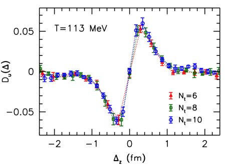
where we employed the same normalization as in the definition (5) of . The ratio represents the correlation between the topological charge density and the electric charge density at two distinct points separated by a four-vector . We remark that in our Euclidean setting, the correlator in the numerator of Eq. (11) is imaginary. Since the observable contains no dependence on the (imaginary) time, its analytic continuation simply amounts to a multiplication by , giving a real observable in Minkowski space-time555 To see this, note that the density of topological charge receives a factor of via the continuation. Furthermore, the Minkowskian Dirac matrices are given by , , such that the charge operator is the same in both space-times. Altogether, the observable gets multiplied by . The same continuation for the observable gives no imaginary factor, since the spin operator in Minkowski space-time is defined as , such that and . . In the left panel of Fig. 4 we show this correlator for the up quark in the plane. The figure reveals an excess of positive charge above () the topological ‘source’ and an excess of negative charge below () it. Thus, we indeed observe an electric dipole structure aligned with the magnetic field.
To show that this spatially separated electric charge is not a lattice artefact, in the right panel of Fig. 4 we plot for . To approach the continuum limit in a well-defined manner, we again make use of the gradient flow and consider a nonzero smearing range. The results using three lattice spacings and lie almost perfectly on top of each other, showing small discretization errors and a fast scaling towards – similarly as we observed for , compare Fig. 3. For the strange quark (which exhibits a better signal to noise ratio) we also considered the dependence of the spatial integral – corresponding to the electric dipole moment of the configuration – on the smearing range. The results indicate that this integral remains nonzero even in the limit . Altogether, we conclude that the spatial separation of the electric charge remains a well-defined concept in the continuum limit.

5 Comparison to a model
Let us now interpret our result for in a model and in the context of heavy-ion collisions. It is instructive to think of the quark-gluon plasma as depicted in the right panel of Fig. 1, with small independent domains containing gluon backgrounds of topological charge . In each domain an electric polarization is induced by the magnetic field and by the local . This can be compared to the magnetic polarization , which is uniform in the whole volume. Let us further assume that the topological charge in each domain is created by constant selfdual or antiselfdual non-Abelian fields of strength , such that . This is a generalization of the approach in Ref. Basar:2011by that allows to describe the case as well as . Like in Ref. Basar:2011by , both polarizations in the local domain can be calculated analytically, when other gluonic interactions are neglected. The calculation (for technical details, see App. B) simplifies tremendously in the lowest-Landau-level (LLL) approximation, which amounts to neglecting the quark masses compared to the field strengths. The magnetic field-dependence of the polarizations then reads
| (12) |
where an identical proportionality factor has been neglected. This result is valid for one quark flavor (whose electric charge is set to unity) and gauge group SU(2) for spatially aligned Abelian and non-Abelian fields, and agrees with the calculation of Ref. Basar:2011by . (Note that Eq. (12) does not hold for where the LLL approximation is invalid. In fact, in this limit vanishes but remains finite.) In App. B we also discuss the case of non-aligned fields and gauge group resulting in similar formulae.
Based on our lattice results, we can make two important statements about this model. First, the ratio is found to be -independent for QCD with physical quark masses in the relevant range of magnetic fields, cf. the left panel of Fig. 2. The equivalent of this quantity in one domain in the model treatment is , which is independent of – and, thus, reproduces the lattice findings – only if the non-Abelian scale exceeds the external field . Second, in this regime (), we may compare the model prediction to the lattice results quantitatively. In order to compute the coefficient in the model, we need to assume a distribution of the topological charge among the local domains. A reasonable approximation is a Gaussian average666 A possible improvement of the model is to take into account correlations between the topological domains, similarly as in phenomenological instanton approaches, see, e.g., Ref. Schafer:1996wv . This might distort the Gaussian distribution of . over . In addition, we also consider an arbitrary angle between the non-Abelian and Abelian fields and integrate over . This averaging over and over is denoted by . Using Eq. (12) for and its generalization to non-aligned fields, Eq. (41) – which we derived for – we obtain
| (13) |
where is a -independent factor describing the dependence of the polarizations on the angle. Its average over cancels in the ratio . In fact, the above obtained number is independent of the width of the Gaussian distribution of (due to the matching powers of in the numerator and the denominator). However, it differs from our lattice determination by an order of magnitude. Put differently, the strong interaction between quarks prevents their full polarization predicted by such a model.
The above comparison reveals that an effective description of QCD with magnetic fields has to take the strong interaction into account non-perturbatively and beyond the simple assumptions of this model. In the same spirit one can question the lowest-Landau-level approximation used in the model setting. It corresponds to the idealized situation where the quark mass vanishes, and all quarks which are spin polarized by the magnetic field interact with the gluonic background and contribute to the electric polarization. However, heavier quarks are less sensitive to topology, and, accordingly, we expect the ratio to decrease as grows. This is consistent with our results .
6 Summary
Using first principles lattice calculations, we have studied local CP violation in the QCD vacuum and its relation to the chiral magnetic effect, and determined the correlation coefficient between the electric polarization and the topological charge density, induced by an external magnetic field. We have considered flavor QCD with physical quark masses, and extrapolated the results to the continuum limit. Our main result is a steady linear dependence of this correlation on (without an indication of saturation) for magnetic fields , covering the maximal magnetic fields estimated to be present in heavy-ion collisions. The coefficient of proportionality – after a normalization by the magnetic polarization, see Eq. (5) – is obtained to be . The results for the three flavors , at two different temperatures are listed in Tab. 1.
We also estimated this coefficient using a model calculation employing nearly massless quarks, the lowest-Landau-level approximation and constant selfdual gluon backgrounds. This model was found to overestimate by an order of magnitude. In other words, there is a substantial quantitative difference of the strength of local CP-violation for quasi-free quarks used in model approaches and fully interacting quarks in realistic physical situations. Whether the electric current in the formulation of the CME with a chiral chemical potential Fukushima:2008xe is also subject to a similar suppression due to non-perturbative QCD effects (first lattice results indicate a suppression by a factor of 3–4 Yamamoto:2011gk ), does not follow directly from our results. However, we take the results as a hint that effects due to local CP-violation in general contain similar suppression factors.
Let us finally add that we employed the staggered discretization of the QCD quark action in the lattice simulation, which in some topology-related aspects gives rise to large systematic/discretization errors. The topological susceptibility, , for example, shows a rather slow scaling towards the continuum limit, see, e.g., Ref. Bazavov:2010xr . We find that for our particular observable, , the continuum extrapolation is much flatter. This may have to do with the fact that is a local observable whereas the susceptibility is not. Nevertheless, it would be desirable to confirm our numerical findings with chiral fermions that have nicer topological properties.
Acknowledgements.
This work was supported by the DFG (SFB/TRR 55, BR 2872/6-1), the EU (ITN STRONGnet 238353 and ERC No 208740) and the Alexander von Humboldt Foundation. The authors would like to thank Pavel Buividovich, Maxim Chernodub, Tigran Kalaydzhyan, Berndt Müller and Kálmán Szabó for useful discussions.Appendix A Details of the gradient flow
The smearing of the gluonic and fermionic fields is performed by evolving these fields in flow time ( is the physical flow time). The evolution in flow time amounts to finding the solution of the flow equations for the gluonic links Luscher:2010iy ,
| (14) |
and for the quark fields Luscher:2013cpa ,
| (15) |
and the corresponding equation for . Here, is the (algebra-valued) derivative of the plaquette action with respect to the link variable, and is the lattice discretization of the Laplace operator (see below). The solution of the flow equations can be found by numerical integration, which is done using the third-order Runge-Kutta integrator described in Refs. Luscher:2010iy ; Luscher:2013cpa (a stepsize of was found to be optimal here, see also Ref. Borsanyi:2012zs ). Integrating the flow equations up to a fixed physical time corresponds to a smearing of the fields over a range of Luscher:2010iy .
The definition of the quark condensate – or, of the fermionic bilinears appearing in Eq. (5) – at nonzero flow time requires the use of the adjoint flow for the noisy estimators of Eq. (9) from flow time back to flow time , see Ref. Luscher:2013cpa . For this, an optimal scheme for the storage of the evolved links for is implemented. The evolution along the gradient flow is started from our original gauge action, thus with unsmeared links. The stout smearing is then applied only for the measurement of the operators, see Eqs. (7)–(9).
We remark that there is a peculiar issue that arises if one applies the fermionic gradient flow for staggered quarks in a naive way. In the staggered fermionic discretization, the Dirac components of the quark field at site are distributed over vertices of the four-dimensional hypercube touching . This distribution of the components is devised in a manner such that the staggered action becomes diagonal in Dirac space, and the only remnant of the original Dirac structure is through space-dependent real numbers, the so-called staggered phases. In particular, the mass term and the Dirac operator are diagonal in Dirac space, therefore they can be represented in terms of the staggered quark fields in the same form, e.g. . However, the naive discretization of the Laplace operator is not diagonal after the staggered transformation, giving no straightforward correspondence between the representation with the original fields and that with the staggered fields.
To construct the Laplacian, let us define the forward and backward covariant difference operators,
| (16) |
where are the gluonic links and the phases corresponding to the magnetic field. The naive one-step discretization of the Laplace operator, indeed becomes off-diagonal as it mixes the tastes distributed over the hypercube in a non-trivial way. One possibility to avoid this mixing of the tastes is to use the two-step discretization of the covariant differences,
| (17) |
to define the Laplacian . This two-step discretization was used in the flow equation Eq. (15). The non-diagonal nature of results in an explicit Lorentz-symmetry breaking of the evolved fermionic fields, even at . This is indicated by asymmetric expectation values of the bilinear structures . Using the two-step Laplacian , (the lattice discretized version of) Lorentz-symmetry is maintained, and for all .
Finally we remark that we also attempted to use the square of the staggered Dirac operator in place of the Laplacian for the evolution of the fermionic fields in Eq. (15). The results obtained for the coefficient after the flow with , however, showed an inferior scaling towards , as compared to the case with . Performing the extrapolation to the continuum limit was only feasible for the latter choice.
Appendix B Polarizations in topological backgrounds
In order to evaluate in a topological background, we consider one quark flavor in constant commuting selfdual or antiselfdual non-Abelian fields, which exist in a finite Euclidean box with quantized fluxes 'tHooft:1981sz (they can also be thought of as fields deep inside instantons or antiinstantons Basar:2011by ) plus an Abelian magnetic field . In these backgrounds, both the topological charge and the polarizations and are constant in space. The quark mass is denoted by and the electric charge is set to unity for simplicity. Moreover, our notation is such that the QCD coupling does not enter the covariant derivative. We follow two equivalent approaches to determine the electric and magnetic polarizations in this model setting. First we employ a spectral representation of the observables using Landau-levels. Second we write down the polarizations using the exact quark propagator in the specific background.
B.1 Polarizations using the spectral representation
Let us first consider the case where the non-Abelian field is (anti)parallel to the Abelian one . Without loss of generality we can assume that points in the direction. Taking for the non-Abelian group, the and components of the total field strength read
| (18) |
where we diagonalized the field strengths via a gauge transformation (for constant field strengths this is always possible). We also inserted the sign of the topological charge in the electric components to account for both the selfdual and the anti-selfdual cases. Let us first discuss the upper color component and denote and . The Dirac eigenvalues of this system are obtained through two independent Landau-level problems in the - and -planes (the arrows indicate the eigenvalues of the corresponding operators),
| (19) |
with and . The spin polarizations read Bali:2012jv
| (20) |
where is the degeneracy of all Landau-levels. The spin-dependence is such that only the corresponding lowest Landau-levels contribute: for , whereas for , cf. App. B in Ref. Bali:2012jv , giving
| (21) |
Note that the polarizations change sign when their corresponding field strengths or are reversed, as they should. The sum in contains an - and -independent divergence,
| (22) |
which we separated using zeta function regularization (here, is the polygamma function of order ). The corresponding divergent contributions in the polarizations are linear in the field and can be absorbed into the renormalization of the electric charge777 Note that this is unnecessary for since the divergence linear in cancels against the contribution of the second color sector, where , see Eq. (18). For no such cancellation takes place since the magnetic field contains an Abelian component which is not traceless. . After this subtraction, the leading term of the second contribution in Eq. (22) in the limit equals . It flips the sign of the first term in Eq. (22) and, thus, for small masses indeed coincides with the lowest-Landau-level contribution, obtained by simply putting , in (21). Hence,
| (23) |
To calculate the full polarizations, we add the contributions of all color components in Eq. (18),
| (24) |
arriving at Eq. (12) used in Sec. 5. The first and third lines agree with Eqs. (81) and (82) of Ref. Basar:2011by , while the second line can also be obtained from the number of zero modes, Eq. (47) of that reference. Note that at , where would have a cusp, the lowest-Landau-level approximation breaks down in the color sector with field strength .
We now turn to the gauge group . One can again diagonalize the field strength, now it has two independent amplitudes in the fields in three color sectors, and . This slightly complicates the calculations. For the simplest case of space-parallel fields in the lowest Landau-level approximation one gets, in analogy to (23)–(24)
| (25) |
We have found that the ratio is -independent and equals when all three fields , and are large compared to , and that it is smaller and becomes -dependent if one of them is not.
B.2 Polarizations using the exact propagator
We proceed by generalizing the above calculation and allow for an arbitrary polar angle between the non-Abelian and Abelian fields,
| (26) |
This case should be equally relevant for estimating in realistic QCD configurations. We again considered the selfdual and the antiselfdual cases simultaneously by inserting in the electric fields.
It is now advantageous to represent the polarizations (first we discuss a single color sector) by
| (27) |
where is the Green’s function of the Dirac operator in the presence of a constant Abelian field and the trace contains a sum over spinor indices and an average over space-time. The latter is trivial since the field strength and also the polarizations are constant. For the Green’s function we employ the proper time representation Schwinger:1951nm ,
| (28) |
where we have moved the integration contour from (just below) the real axis to the negative imaginary axis parameterizing the original integration variable as . Here, indicates terms that vanish under the Dirac trace in Eq. (27), and the sign of the term containing is chosen such that it conforms to the definition (2). Moreover, we introduced
| (29) |
viewing as an antisymmetric tensor in Lorentz indices (having purely imaginary eigenvalues).
Let us denote the invariants of (proportional to ‘action’ and ‘topological charge’ density) as
| (30) |
Then the eigenvalues are given by Schwinger:1951nm
| (31) |
with and . The determinant of is simply . The eigenvalues come in pairs with opposite signs, in accordance with the tracelessness of , and the arguments of the square roots in them are all positive. Using this we obtain
| (32) |
By explicit comparison we found that the other factor appearing in can be represented as
| (33) |
For our situation these quantities read
| (34) | ||||
| (35) |
and in terms of
| (36) |
the projections become
| (37) |
The second line confirms that changes sign if the topological charge does so.
Plugging all this into the proper time integral (28) shows that the integral diverges as . This is the same divergence that we encountered in Eq. (22). Here we eliminate it by dividing the observable by and differentiating it with respect to , cf. Eq. (21). This indeed renders the integral finite and also reveals that the divergence is independent of and of the fields. Setting (and consequently etc.) reproduces the finite part of Eq. (22).
For , two hyperbolic sine functions are left in the denominator of Eq. (32), such that the proper time integral cannot be performed easily. Since we argued that the region (i.e. for all ) is the relevant one for comparison with the lattice data, we now specialize to this case. Then and the proper time integral reads888 In the general case one has to use instead of in the denominator of Eq. (38).
| (38) |
Similarly as in Eq (23), we now resort to the approximation . Moreover, in order to simplify the integral, we also assume . Expanding the fraction in and , we can perform the -integral to arrive at
| (39) |
Notice that the term in Eq. (38) does not contribute at this order, which, using Eq. (37), implies that . Using the expansion and gives
| (40) |
Here the leading term vanishes upon adding the second color sector of , which amounts to the same expression with , cf. Eq. (24). Adding the contributions of both sectors and integrating in we finally get
| (41) |
which, at , reproduces Eq. (24) for the case . This expression was inserted in Eq. (13). Note that the average over the polar angle factorizes and gives
| (42) |
References
- (1) Y. Aoki, G. Endrődi, Z. Fodor, S. Katz, and K. Szabó, The Order of the quantum chromodynamics transition predicted by the standard model of particle physics, Nature 443 (2006) 675–678, [hep-lat/0611014].
- (2) Y. Aoki, Z. Fodor, S. Katz, and K. Szabó, The QCD transition temperature: Results with physical masses in the continuum limit, Phys.Lett. B643 (2006) 46–54, [hep-lat/0609068].
- (3) Wuppertal-Budapest Collaboration, S. Borsányi et. al., Is there still any mystery in lattice QCD? Results with physical masses in the continuum limit III, JHEP 1009 (2010) 073, [arXiv:1005.3508].
- (4) PHENIX Collaboration, A. Adare et. al., Detailed measurement of the pair continuum in and Au+Au collisions at GeV and implications for direct photon production, Phys. Rev. C81 (2010) 034911, [arXiv:0912.0244].
- (5) V. Skokov, A. Y. Illarionov, and V. Toneev, Estimate of the magnetic field strength in heavy-ion collisions, Int. J. Mod. Phys. A24 (2009) 5925–5932, [arXiv:0907.1396].
- (6) T. Vachaspati, Magnetic fields from cosmological phase transitions, Phys. Lett. B265 (1991) 258–261.
- (7) R. C. Duncan and C. Thompson, Formation of very strongly magnetized neutron stars - implications for gamma-ray bursts, Astrophys. J. 392 (1992) L9.
- (8) D. Kharzeev, R. Pisarski, and M. H. Tytgat, Possibility of spontaneous parity violation in hot QCD, Phys.Rev.Lett. 81 (1998) 512–515, [hep-ph/9804221].
- (9) D. E. Kharzeev, L. D. McLerran, and H. J. Warringa, The Effects of topological charge change in heavy ion collisions: ’Event by event P and CP violation’, Nucl.Phys. A803 (2008) 227–253, [arXiv:0711.0950].
- (10) K. Fukushima, D. E. Kharzeev, and H. J. Warringa, The Chiral Magnetic Effect, Phys. Rev. D78 (2008) 074033, [arXiv:0808.3382].
- (11) D. Kharzeev, Parity violation in hot QCD: Why it can happen, and how to look for it, Phys.Lett. B633 (2006) 260–264, [hep-ph/0406125].
- (12) S. A. Voloshin, Parity violation in hot QCD: How to detect it, Phys.Rev. C70 (2004) 057901, [hep-ph/0406311].
- (13) STAR Collaboration, S. A. Voloshin, Probe for the strong parity violation effects at RHIC with three particle correlations, Indian J.Phys. 85 (2011) 1103–1107, [arXiv:0806.0029].
- (14) STAR Collaboration, B. Abelev et. al., Azimuthal Charged-Particle Correlations and Possible Local Strong Parity Violation, Phys.Rev.Lett. 103 (2009) 251601, [arXiv:0909.1739].
- (15) ALICE Collaboration, I. Selyuzhenkov, Anisotropic flow and other collective phenomena measured in Pb-Pb collisions with ALICE at the LHC, Prog.Theor.Phys.Suppl. 193 (2012) 153–158, [arXiv:1111.1875].
- (16) F. Wang, Effects of Cluster Particle Correlations on Local Parity Violation Observables, Phys.Rev. C81 (2010) 064902, [arXiv:0911.1482].
- (17) B. Müller and A. Schäfer, Charge Fluctuations from the Chiral Magnetic Effect in Nuclear Collisions, Phys.Rev. C82 (2010) 057902, [arXiv:1009.1053].
- (18) V. Voronyuk, V. Toneev, W. Cassing, E. Bratkovskaya, V. Konchakovski, et. al., (Electro-)Magnetic field evolution in relativistic heavy-ion collisions, Phys.Rev. C83 (2011) 054911, [arXiv:1103.4239].
- (19) A. Bzdak, V. Koch, and J. Liao, Charge-Dependent Correlations in Relativistic Heavy Ion Collisions and the Chiral Magnetic Effect, Lect.Notes Phys. 871 (2013) 503–536, [arXiv:1207.7327].
- (20) K. Fukushima, Views of the Chiral Magnetic Effect, Lect.Notes Phys. 871 (2013) 241–259, [arXiv:1209.5064].
- (21) D. E. Kharzeev, The Chiral Magnetic Effect and Anomaly-Induced Transport, arXiv:1312.3348.
- (22) K. Fukushima, M. Ruggieri, and R. Gatto, Chiral magnetic effect in the PNJL model, Phys.Rev. D81 (2010) 114031, [arXiv:1003.0047].
- (23) H.-U. Yee, Holographic Chiral Magnetic Conductivity, JHEP 0911 (2009) 085, [arXiv:0908.4189].
- (24) A. Rebhan, A. Schmitt, and S. A. Stricker, Anomalies and the chiral magnetic effect in the Sakai-Sugimoto model, JHEP 1001 (2010) 026, [arXiv:0909.4782].
- (25) V. I. Zakharov, Chiral Magnetic Effect in Hydrodynamic Approximation, Lect.Notes Phys. 871 (2013) 295–330, [arXiv:1210.2186].
- (26) T. Kalaydzhyan, Chiral superfluidity of the quark-gluon plasma, Nucl.Phys. A913 (2013) 243–263, [arXiv:1208.0012].
- (27) Z. Khaidukov, V. Kirilin, A. Sadofyev, and V. Zakharov, On Magnetostatics of Chiral Media, arXiv:1307.0138.
- (28) P. Buividovich, M. Chernodub, E. Luschevskaya, and M. Polikarpov, Numerical evidence of chiral magnetic effect in lattice gauge theory, Phys.Rev. D80 (2009) 054503, [arXiv:0907.0494].
- (29) V. Braguta, P. Buividovich, T. Kalaydzhyan, S. Kuznetsov, and M. Polikarpov, The Chiral Magnetic Effect and chiral symmetry breaking in SU(3) quenched lattice gauge theory, PoS LATTICE2010 (2010) 190, [arXiv:1011.3795].
- (30) A. Yamamoto, Chiral magnetic effect in lattice QCD with a chiral chemical potential, Phys.Rev.Lett. 107 (2011) 031601, [arXiv:1105.0385].
- (31) P. Buividovich, Anomalous transport with overlap fermions, arXiv:1312.1843.
- (32) M. Abramczyk, T. Blum, G. Petropoulos, and R. Zhou, Chiral magnetic effect in 2+1 flavor QCD+QED, PoS LAT2009 (2009) 181, [arXiv:0911.1348].
- (33) P. Buividovich, M. Chernodub, E. Luschevskaya, and M. Polikarpov, Quark electric dipole moment induced by magnetic field, Phys.Rev. D81 (2010) 036007, [arXiv:0909.2350].
- (34) M. Lüscher, Properties and uses of the Wilson flow in lattice QCD, JHEP 1008 (2010) 071, [arXiv:1006.4518].
- (35) G. Basar, G. V. Dunne, and D. E. Kharzeev, Electric dipole moment induced by a QCD instanton in an external magnetic field, Phys.Rev. D85 (2012) 045026, [arXiv:1112.0532].
- (36) B. L. Ioffe and A. V. Smilga, Nucleon Magnetic Moments and Magnetic Properties of Vacuum in QCD, Nucl. Phys. B232 (1984) 109.
- (37) E. Witten, Dyons of Charge e theta/2 pi, Phys.Lett. B86 (1979) 283–287.
- (38) S. Borsányi, G. Endrődi, Z. Fodor, A. Jakovác, S. D. Katz, et. al., The QCD equation of state with dynamical quarks, JHEP 1011 (2010) 077, [arXiv:1007.2580].
- (39) S. Borsányi, Z. Fodor, C. Hoelbling, S. D. Katz, S. Krieg, et. al., Full result for the QCD equation of state with 2+1 flavors, arXiv:1309.5258.
- (40) Y. Aoki, Z. Fodor, S. D. Katz, and K. K. Szabó, The equation of state in lattice QCD: With physical quark masses towards the continuum limit, JHEP 01 (2006) 089, [hep-lat/0510084].
- (41) G. Bali, F. Bruckmann, G. Endrődi, Z. Fodor, S. Katz, et. al., The QCD phase diagram for external magnetic fields, JHEP 1202 (2012) 044, [arXiv:1111.4956].
- (42) T. A. DeGrand, A. Hasenfratz, and T. G. Kovács, Topological structure in the SU(2) vacuum, Nucl.Phys. B505 (1997) 417–441, [hep-lat/9705009].
- (43) G. Bali, F. Bruckmann, M. Constantinou, M. Costa, G. Endrődi, et. al., Magnetic susceptibility of QCD at zero and at finite temperature from the lattice, Phys.Rev. D86 (2012) 094512, [arXiv:1209.6015].
- (44) F. Bruckmann, F. Gruber, N. Cundy, A. Schäfer, and T. Lippert, Topology of dynamical lattice configurations including results from dynamical overlap fermions, Phys. Lett. B707 (2012) 278, [arXiv:1107.0897].
- (45) M. Lüscher, Chiral symmetry and the Yang–Mills gradient flow, JHEP 1304 (2013) 123, [arXiv:1302.5246].
- (46) G. Bali, F. Bruckmann, G. Endrődi, Z. Fodor, S. Katz, et. al., QCD quark condensate in external magnetic fields, Phys.Rev. D86 (2012) 071502, [arXiv:1206.4205].
- (47) F. Bruckmann, G. Endrődi, and T. G. Kovács, Inverse magnetic catalysis and the Polyakov loop, JHEP 1304 (2013) 112, [arXiv:1303.3972].
- (48) G. Bali, F. Bruckmann, G. Endrődi, F. Gruber, and A. Schäfer, Magnetic field-induced gluonic (inverse) catalysis and pressure (an)isotropy in QCD, JHEP 1304 (2013) 130, [arXiv:1303.1328].
- (49) G. Bali, K. Schilling, J. Fingberg, U. M. Heller, and F. Karsch, Computation of the spatial string tension in high temperature SU(2) gauge theory, Int.J.Mod.Phys. C4 (1993) 1179–1193, [hep-lat/9308003].
- (50) S. Dürr, Z. Fodor, J. Frison, C. Hoelbling, R. Hoffmann, et. al., Ab-Initio Determination of Light Hadron Masses, Science 322 (2008) 1224–1227, [arXiv:0906.3599].
- (51) T. Schäfer and E. V. Shuryak, Instantons in QCD, Rev.Mod.Phys. 70 (1998) 323–426, [hep-ph/9610451].
- (52) MILC Collaboration, A. Bazavov et. al., Topological susceptibility with the asqtad action, Phys.Rev. D81 (2010) 114501, [arXiv:1003.5695].
- (53) S. Borsányi, S. Dürr, Z. Fodor, C. Hoelbling, S. D. Katz, et. al., High-precision scale setting in lattice QCD, JHEP 1209 (2012) 010, [arXiv:1203.4469].
- (54) G. ’t Hooft, Some Twisted Selfdual Solutions for the Yang-Mills Equations on a Hypertorus, Commun.Math.Phys. 81 (1981) 267–275.
- (55) J. S. Schwinger, On gauge invariance and vacuum polarization, Phys.Rev. 82 (1951) 664–679.