Generalized belief propagation for the magnetization of the simple cubic Ising model

Abstract

A new approximation of the cluster variational method is introduced for the three–dimensional Ising model on the simple cubic lattice. The maximal cluster is, as far as we know, the largest ever used in this method. A message–passing algorithm, generalized belief propagation, is used to minimize the variational free energy. Convergence properties and performance of the algorithm are investigated.

The approximation is used to compute the spontaneous magnetization, which is then compared to previous results. Using the present results as the last step in a sequence of three cluster variational approximations, an extrapolation is obtained which captures the leading critical behaviour with a good accuracy.

1 Introduction

A major approximate tool in the equilibrium statistical physics of lattice models is the mean–field theory, together with its many generalizations. These techniques are known to give quite often reliable qualitative results, which makes them very useful in understanding properties of a model like its phase diagram. Due to the limited quantitative accuracy of simple mean–field theory, many generalizations were developed. Since mean–field neglects correlations, typically the idea is to include local, but progressively longer range correlations in the treatment, for example by means of cluster expansions where clusters of increasing size can be included.

This line of research started with the Bethe–Peierls approximation [1, 2], where nearest–neighbour correlations are taken into account, and the Kramers–Wannier approximation [3, 4], including correlations up to a square plaquette. Many generalizations were then proposed, and a particularly successful one was the cluster variational method (CVM), introduced by Kikuchi in 1951 [5] and applied to the Ising model. The largest clusters considered by Kikuchi in this work were a cube of 8 sites for the simple cubic lattice and a tetrahedron of 4 sites for the face centered cubic lattice.

Larger clusters were later considered: in 1967 Kikuchi and Brush [9] introduced the $B_{2L}$ sequence of approximations for the two–dimensional square lattice, whose convergence properties were later studied [10] using maximal clusters up to 13 sites. Kikuchi and Brush also suggested that a similar approach could in principle be carried out in three dimensions, although the computational costs would have been prohibitively large at that time. Their intuition was put on a firmer ground by Schlijper [6, 7, 8], who showed that, for translation–invariant models in the thermodynamical limit, there exist sequences of CVM approximations whose free energy converges to the exact one. For a $d$–dimensional model, the largest clusters to consider grow in $d-1$ dimensions only, as in a transfer matrix approach. In 3 dimensions this idea was used by the present author to develop a CVM approximation for the Ising model on the simple cubic lattice based on an 18–site ($3\times 3\times 2$) cluster [11].

The main difficulty encountered in trying to enlarge the basic clusters is the computational cost, which grows exponentially with the cluster size. More precisely the problem can be written as the minimization of a free energy whose number of indipendent variables increases exponentially with the cluster size. A significant amount of work was then devoted to develop efficient algorithms. The original iterative algorithm proposed by Kikuchi [12, 13, 14], the so–called natural iteration method, is not particularly efficient, but in certain cases it is provably convergent [15] to a (maybe local) minimum of the free energy. Faster, provably convergent algorithms were developed more recently [16, 17].

A very important step in the direction of speeding up algorithms for the minimization of the CVM free energy has been made in 2001, when it was shown [18] that Belief Propagation (BP) [19], a message–passing algorithm widely used for approximate inference in probabilistic graphical models, is strictly related to the Bethe–Peierls approximation. In particular, it was shown [18] that fixed points of the BP algorithms correspond to stationary points of the Bethe–Peierls variational free energy. This result was later extended by showing that stable fixed points of BP are (possibly local) minima of the Bethe–Peierls variational free energy, though the converse is not necessarily true. This provides us with the fastest, but not always convergent, algorithm for the minimization of the Bethe–Peierls free energy. When convergent, BP outperforms the other algorithms by orders of magnitude (see [10] for a detailed comparison). BP was also extended to an algorithm, named Generalized Belief Propagation (GBP) [18, 20], whose fixed points are stationary points of the CVM free energy for any choice of basic clusters. Like BP, GBP is extremely fast but not always convergent.

The purpose of the work described here is twofold: we aim both to test how GBP performs in minimizing a CVM free energy with a very large (32 sites) basic cluster, and to make one more step in the hierarchy of CVM approximations for three–dimensional lattice models. Working on the Ising model on the simple cubic lattice as a paradigmatic example, we follow Schlijper’s ideas and enlarge the basic cluster for our CVM approximation in 2 dimensions only, thus choosing a $4\times 4\times 2$ cluster (as far as we know, the largest cluster ever considered in CVM). We then use a GBP algorithm to minimize the corresponding free energy in a wide range of temperatures and discuss the accuracy of the result, focussing in particular on the spontaneous magnetization, in comparison with state–of–the–art results.

The paper is organized as follows: in Sec. 2 we describe our CVM approximation and the GBP algorithm we use to minimize it, in Sec. 3 we analyze the performance of the algorithm and the accuracy of the results for the magnetization, and conclusions are drawn in Sec. 4.

2 Methodology

The CVM is based on the minimization of an approximate variational free energy, which is obtained from a truncation of a cumulant expansion of the entropy [6, 10, 21, 22, 23]. A particular CVM approximation is specified by the set $R$ of clusters one wants to keep in the expansion: the typical choice involves a set of maximal clusters and all their subclusters. Introducing the Möbius numbers $\{a_{\alpha},\alpha\in R\}$, defined by

$$\sum_{\beta\subseteq\alpha\in R}a_{\alpha}=1\qquad\forall\beta\in R,$$ (1)

the variational free energy takes the form

$${\cal F}(\{p_{\alpha},\alpha\in R\})=\sum_{\alpha\in R}a_{\alpha}{\cal F}_{\alpha}(p_{\alpha}).$$ (2)

Here $p_{\alpha}$ is the probability distribution for cluster $\alpha$ and

$${\cal F}_{\alpha}(p_{\alpha})=\sum_{{s_{\alpha}}}\left[p_{\alpha}({s_{\alpha})}H_{\alpha}({s_{\alpha}})+Tp_{\alpha}({s_{\alpha})}\ln p_{\alpha}({s_{\alpha})}\right],$$ (3)

where $s_{\alpha}=\{s_{i},i\in\alpha\}$ is the configuration of cluster $\alpha$, $H_{\alpha}$ its contribution to the Hamiltonian and, as customary, $T$ is the absolute temperature (Boltzmann’s constant $k_{B}$ has been set to 1). If $H$ is the Hamiltonian of the model under consideration, then the condition

$$H=\sum_{\alpha\in R}a_{\alpha}H_{\alpha}(s_{\alpha})$$ (4)

must be satisfied. In the following we shall consider the nearest–neighbour Ising model in zero field, so our Hamiltonian will be

$$H=-\sum_{\langle ij\rangle}s_{i}s_{j},\qquad s_{i}=\pm 1$$ (5)

(the coupling constant $J$ has also been set to 1, hence the temperature will be expressed in units of $J/k_{B}$). The splitting of $H$ into contributions $H_{\alpha}$ from the various clusters appearing in the expansion is not unique, several (equivalent) choices are possible. In the following we distribute $H$ evenly among the maximal clusters only, so that no Hamiltonian terms appear in the subcluster free energies.

Our choice for the largest clusters in $R$ is based on Schlijper’s result [6, 7, 8] that for a $d$–dimensional model one can improve accuracy by increasing the maximal clusters in $d-1$ dimensions only. On the simple cubic lattice, the elementary cubic cell of $2\times 2\times 2$ sites has been already considered by Kikuchi [5] and a $3\times 3\times 2$ basic cluster made of 4 elementary cubic cells has been used in [11]. The next step in this sequence is then a $4\times 4\times 2$ basic cluster (32 sites, 9 elementary cubic cells). As far as we know, this is the largest maximal cluster ever used in a CVM approximation. The number of possible Ising configurations of such a cluster is $2^{32}\simeq 4\cdot 10^{9}$, which is also the number of independent variables in our variational problem. More precisely, exploiting lattice symmetries, this number can be reduced by a factor close to 16, leaving us with $\simeq 2^{28}\simeq 2.5\cdot 10^{8}$ independent variables. In order to deal with such a large number of variables, we shall use the parent–to–child GBP algorithm [20] to find stationary points of the variational free energy. This will also provide a test of convergence and performance of the algorithm in a very large scale problem.

The parent–to–child GBP algorithm is a message–passing algorithm, based on iterative equations written in terms of quantities called messages, which are exchanged between clusters. We shall use the notation $m_{\alpha\to\beta}(s_{\beta})$ for a message going from cluster $\alpha$ to cluster $\beta$, which is a function of the configuration $s_{\beta}$ of the latter. Only clusters $\alpha\in R$ with Möbius number $a_{\alpha}\neq 0$ are involved in the message–passing scheme. Exploiting the lattice translational invariance in the thermodynamic limit, we shall identify a cluster by the symbol $l_{x}l_{y}l_{z}$, where $l_{x}$, $l_{y}$ and $l_{z}$ are the lengths of the cluster in the three spatial directions, in terms of lattice sites. For instance, a cluster made of a single site will be denoted by 111, nearest–neighbour pairs in the three directions by 211, 121 and 112 respectively, the elementary cubic cell by 222, and our maximal cluster by 442. With this notation, it is easy to check that, according to Eq. 1, if $R$ includes 442 and all its subclusters, the only clusters with non–vanishing Möbius numbers are the following:

$$a_{442}=1 a_{432}=a_{342}=-1 a_{332}=1$$

$$a_{441}=-1 a_{431}=a_{341}=1 a_{331}=-1.$$ (6)

Thanks to lattice isotropy, when $l_{x}\neq l_{y}$, the clusters $l_{x}l_{y}l_{z}$ and $l_{y}l_{x}l_{z}$ are equivalent, so we need to consider only six different clusters, that is six probability distributions, related to each other by marginalization conditions. In the parent–to–child GBP algorithm [20], messages go from a (parent) cluster $\alpha$ to a direct subcluster (child) $\beta\subset\alpha$, where direct means that there exist no other cluster $\gamma$ with $a_{\gamma}\neq 0$ such that $\beta\subset\gamma\subset\alpha$. Hence, in the present CVM approximation, we will have to introduce only the messages corresponding to the parent–child pairs listed in Tab. 1.

Parent	Child
431	331
441	431
432	332
442	432
332	331
432	431
442	441

Table 1: Parent–child pairs for messages in the parent–to–child GBP algorithm for our CVM approximation

In the parent–to–child GBP algorithm [20], cluster probability distributions at a stationary point of the CVM variational free energy are written in terms of messages (up to a normalization constant) as

$$p_{\gamma}({s_{\gamma}})\propto\exp\left[-H_{\gamma}({s_{\gamma}})\right]\prod_{\beta\subseteq\gamma}\prod_{\beta\subset\alpha\in R}^{\alpha\nsubseteq\gamma}m_{\alpha\to\beta}({s_{\beta}}),$$ (7)

where $s_{\beta}$ denotes the restriction of ${s_{\gamma}}$ to subcluster $\beta$. In the above products $\beta$ is any subcluster of $\gamma$ (including $\gamma$ itself) with $a_{\beta}\neq 0$, while $\alpha$ is any parent of $\beta$ not contained in $\gamma$.

Messages are computed by iterating equations derived from the marginalization conditions which must be fulfilled by the probability distributions of a parent cluster $\alpha$ and one of its children clusters $\beta$:

$$p_{\beta}({s_{\beta})}=\sum_{{s_{\alpha\setminus\beta}}}p_{\alpha}({s_{\alpha}}),$$ (8)

where $s_{\alpha\setminus\beta}=\{s_{i},i\in\alpha\setminus\beta\}$. In the resulting set of equations, messages at (iteration) time $t$ enter the right–hand side and new messages at time $t+1$ are obtained on the left–hand side. Writing down the above equations for all parent–child pairs one realizes that two cases can be distinguished.

As a first example, consider $\beta=331$ and $\alpha=332$ and write the corresponding probability distributions using Eq. 7. It can be easily checked that all messages appearing in the left–hand side, except $m_{\alpha\to\beta}(s_{\beta})$, will appear also in the right–hand side, cancelling each other. The resulting equation will then give (up to a normalization constant) directly $m_{\alpha\to\beta}(s_{\beta})$ as a function of other messages and can be included in an iterative scheme where messages at step $t$ enter the right–hand side and a new value for $m_{\alpha\to\beta}(s_{\beta})$ at time $t+1$ is obtained.

As a second example, consider now $\beta=431$ and $\alpha=432$. In this case, after cancellations, the left–hand side will contain the product of $m_{\alpha\to\beta}(s_{\beta})$ and two more messages, specifically those which go from the 332 subclusters of $\alpha$ to the corresponding 331 subclusters of $\beta$. As a consequence, in order to evaluate new $432\to 431$ messages at time $t+1$, one must have already computed the new $332\to 331$ messages at time $t+1$ from the corresponding equations. By working out the details for all messages a partial order emerges among the various computations. At time $t+1$ one has to compute:

1. first $431\to 331$ messages;

2. then $441\to 431$ and $432\to 332$ (no definite order between them);

3. then $442\to 432$ messages;

and, independent of the above:

1. first $332\to 331$ messages;

2. then $432\to 431$ messages;

3. then $442\to 441$ messages.

We shall close this section with a few technical details about the implementation of the above scheme.

In the GBP algorithm, messages are defined up to a normalization constant. More precisely, for a given $\alpha\to\beta$ parent–child pair, the messages $m_{\alpha\to\beta}(s_{\beta}),\forall s_{\beta}$ can be rescaled by a common constant. As a consequence, in order to check convergence of the iterative scheme, we need to normalize messages properly. Several (equivalent) choices are possible, we normalize them at each iteration by requiring that

$$\sum_{s_{\beta}}m_{\alpha\to\beta}(s_{\beta})=1$$ (9)

for all $\alpha\to\beta$ parent–child pairs.

Iteration proceeds until the condition

$$\Delta=\sum_{s_{\beta}}\left[m_{\alpha\to\beta}^{\rm(new)}(s_{\beta})-m_{\alpha\to\beta}^{\rm(old)}(s_{\beta})\right]^{2}<\epsilon$$ (10)

is met, where new and old denote messages at times $t+1$ and $t$ respectively. The actual value of $\epsilon$ will be specified in the next section, where we discuss the performance of the algorithm.

Finally, as it often occurs with message–passing algorithms, in order to achieve convergence it is necessary to damp the iteration. There is not a unique recipe, and a reasonable tradeoff between convergence and speed must be looked for in any given problem. Here we found that convergence was always achieved by replacing, after each iteration, the new messages with the geometric mean of old and new messages.

3 Results

The parent–to–child GBP algorithm described in the previous section was applied to the simple cubic Ising model in the low–temperature phase. The inverse temperature $K=T^{-1}$ was varied in the range 0.223 to 0.436, with a step $\delta K=0.001$.

A broken–symmetry initialization was used for the messages:

$$m_{\alpha\to\beta}(s_{\beta})=\prod_{i\in\beta}\frac{1+m_{0}s_{i}}{2},$$ (11)

with $m_{0}=0.1$. The equations for the messages were then iterated until the convergence condition Eq. 10, with $\alpha=442$, $\beta=441$ and $\epsilon=10^{-12}$, was met. With this choice of $\alpha$ and $\beta$ the squared distance $\Delta$ in Eq. 10 contains $2^{16}$ terms, so the average rms variation of individual messages at convergence is not larger than $10^{-6}/2^{8}\simeq 4\cdot 10^{-9}$. Of course, any other choice of the $\alpha\to\beta$ parent–child pair (or a combination of all possible parent–child pairs), with a suitable rescaling of $\epsilon$, produces similar results. The convergence criterion is rather strict: as an example, increasing $\epsilon$ to $10^{-9}$ at $K=0.24$ affects the spontaneous magnetization in the 7th decimal place. After a short transient, the squared distance $\Delta$ decreases exponentially with the number of iterations, as illustrated in Fig. 1.

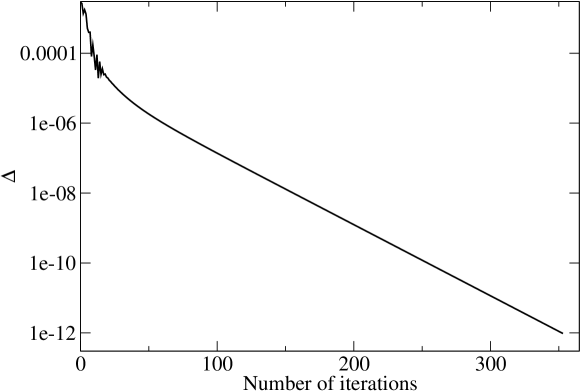
Figure 1: Squared distance $\Delta$ as a function of the number of iterations, for $K=0.223$.

The algoritm converges in a number of iterations $N(K)$ which stays practically constant at 47–48 for $K\geq 0.29$ and exhibits a critical slowing down as the critical temperature is approached. In Fig. 2 we report the number of iterations as a function of $K-K_{c}$, where we have used the estimate $K_{c}\simeq 0.22165$ [24, 25, 26, 27, 28]. It can be clearly seen that $N(K)$ is very well fitted by the function $N_{0}(K-K_{c})^{-z}$, with $z\simeq 0.564$. In the slowest case, $K=0.223$, the algorithm took 354 iterations to converge. The number of messages to be updated at any iteration is mainly determined by the number of $442\to 432$ messages, that is $2^{24}$. Exploiting lattice symmetries this number reduces to $\simeq 2^{22}\sim 4\cdot 10^{6}$. For each message, a sum of $2^{8}$ terms must be evaluated. The time taken by our code to execute a single iteration on a 2.66 GHz, 64 bits single processor is $\simeq 28$ minutes, so the algorithm converges in a time which ranges from approximately 1 day for $K>0.29$ to approximately 1 week at $K=0.223$.

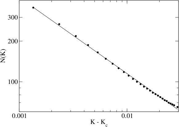
Figure 2: Number of iterations $N(K)$ to reach convergence, as a function of $K-K_{c}$. The solid line is a fit with the function $N_{0}(K-K_{c})^{-z}$.

For each $K$, after convergence, we evaluate the probability distribution of the 331 cluster using Eq. 7, check translational invariance, and compute the spontaneous magnetization $m$. Any correlation function involving a group of sites contained in the 442 cluster can be computed.

In order to assess the accuracy of the method, we have compared our results for the magnetization with the formula by Talapov and Blöte [28], determined on the basis of high precision simulations and finite size scaling. For comparison, we have also considered two lower–order CVM approximation, the cube ($2\times 2\times 2$) one [5] and the 18–site ($3\times 3\times 2$) one [11]. In the following we shall denote by $m_{\rm TB}(K)$ the Talapov–Blöte result and by $m_{L}(K)$ the CVM result from the approximation with the $L\times L\times 2$ maximal cluster, with $L$ going from 2 (the cube approximation) to 4 (the present approximation).

A simple plot of the 4 functions in the critical regions is shown in Fig. 3. The largest deviations occur of course close to the critical point. In particular, at $K=0.223$, the present approximation $m_{4}$ is larger than the Talapov–Blöte estimate $m_{TB}$ by $\simeq 0.018$. Corresponding figures for $m_{3}$ and $m_{2}$ are 0.035 and 0.077 respectively.

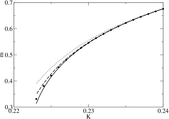
Figure 3: Various estimates of the spontaneous magnetization: Talapov–Blöte $m_{TB}$ (solid line) and $m_{L}$ with $L=4$ (present approximation, filled circles), 3 (dashed line) and 2 (dotted line).

The above result is better appreciated by plotting the deviations $m_{L}(K)-m_{TB}(K)$ from the Talapov–Blöte estimate, reported in Fig. 4. In this figure we also report the deviation $m_{\infty}(K)-m_{TB}(K)$ for an extrapolation $m_{\infty}$. In principle, based on Schlijper’s results [6, 7, 8], for any $K>K_{c}$ one would like to define $m_{\infty}(K)=\displaystyle{\lim_{L\to\infty}}m_{L}(K)$, which should be equal to the exact result. The terms of this sequence for $L>4$ are not available, so we need a finite–size ansatz to extrapolate $m_{\infty}$ from the results for $L=2,3$ and 4. Since for $K>K_{c}$ the model has a characteristic length $\xi(K)$, the correlation length, a natural assumption is that

$$m_{L}(K)=m_{\infty}(K)+\delta m(K)\exp\left[-L/\xi(K)\right],$$ (12)

at least asymptotically. Assuming equality for $L=2,3$ and 4 one finds

$$m_{\infty} = \frac{m_{2}m_{4}-m_{3}^{2}}{m_{2}-2m_{3}+m_{4}}$$ (13)

$$\xi = \left[\log(m_{2}-m_{3})-\log(m_{3}-m_{4})\right]^{-1}.$$ (14)

Notice that $m_{\infty}$ and $\xi$ are independent of an offset which might be added to (or subtracted from) $L$. For example, one could measure the size of the maximal clusters in terms of lattice spacings and obtain $L^{\prime}=1,2$ and 3 for the cube, 18–site and the present approximation, but this would affect only the value of the prefactor $\delta m$. It is also important here to stress that without $m_{4}$ this extrapolation would not have been possible.

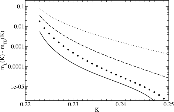
Figure 4: Deviations $m_{L}(K)-m_{TB}(K)$ from Talapov–Blöte estimate, for $L=4$ (present approximation, filled circles), 3 (dashed line), 2 (dotted line) and $\infty$ (extrapolation, solid line).

The correlation length $\xi$ from Eq. 14 is strongly affected by numerical uncertainties, due to the small differences between $m_{2},m_{3}$ and $m_{4}$. Indeed, it oscillates, and then becomes not defined, for $K>0.26$. On the other hand, the extrapolated spontaneous magnetization $m_{\infty}$ does not suffer from these numerical problems and it is remarkably accurate. At $K=0.223$, it is larger than $m_{TB}$ by 0.05 only, less than $1/3$ the corresponding deviation of $m_{4}$. Since $m_{\infty}(K)$ is our best estimate for the spontaneous magnetization, it is worth investigating its critical behaviour. We have fitted our dataset to the function [28]

$$m(t)=t^{\beta}\left(a_{0}-a_{1}t^{\theta}-a_{2}t\right),$$ (15)

where $t=1-K_{c}/K$ denotes reduced temperature, with 6 fitting parameters: $K_{c},\beta,a_{0},a_{1},a_{2},\theta$ (from now on $\beta$ denotes the critical exponent of the spontaneous magnetization), obtaining:

$$K_{c}=0.221510(4),$$

$$\beta=0.332(1),$$

$$a_{0}=1.70(1),$$

$$a_{1}=0.73(7),$$

$$a_{2}=0.03(8),$$

$$\theta=0.72(4).$$

Given the small value of $a_{2}$ we also made a similar fit imposing $a_{2}=0$, with the results

$$K_{c}=0.221512(2),$$

$$\beta=0.3315(3),$$

$$a_{0}=1.694(2),$$

$$a_{1}=0.752(2),$$

$$\theta=0.738(2).$$

For a comparison we recall that Talapov and Blöte best estimate [28], obtained with $K_{c}=0.2216544$, was

$$\beta=0.3269(3),$$

$$a_{0}=1.692(4),$$

$$a_{1}=0.344(6),$$

$$a_{2}=0.426(11),$$

$$\theta=0.508(15).$$

We see that the leading term is captured reasonable well by our approximation, with a slightly smaller $K_{c}$, a slightly larger exponent $\beta$ and a compatible prefactor $a_{0}$, while the same is not true for the correction to scaling terms.

4 Discussion

The present paper discusses the application of the CVM approximation with a $4\times 4\times 2$ maximal cluster to the three–dimensional Ising model on the simple cubic lattice. The maximal cluster is, as far as we know, the largest ever considered (32 sites) and the approximation can be viewed as the third step of a sequence of $L\times L\times 2$ approximations, where $L=2$ is the original cube approximation [5] and $L=3$ was considered in [11].

Due to the large size of the maximal cluster, it is necessary to resort to an instance of the GBP algorithm for the minimization of the variational free energy. As a consequence, this work also tests the GBP algorithm with a very large maximal cluster, showing that convergence can be achieved in reasonable times even with $2^{22}$ messages. The accuracy of the results is assessed by evaluating the spontaneous magnetization and comparing it with previous approximations and with a recent best estimate.

In addition to the expected improvement with respect to $L=2$ and 3, we observe that the availability of results for three $L$ values allows an extrapolation, with the only assumption that the approach to the exact value is exponential in $L$. This assumption is much weaker than those underlying other techniques used to attempt to extrapolate non–classical critical behaviour from generalized mean field theories, like the Cluster Variational – Padé Approximant Method [30, 31] or the Coherent Anomaly Method [32].

The extrapolation gives a good estimate of the leading term of the critical behaviour, although it cannot reach the accuracy of the recent best estimates (see e.g. [29] for a review).

It does not seem feasible, at least at the moment, to investigate the next approximation in the sequence, corresponding to $L=5$. This would mean to use a 50–site maximal cluster, making the number of variables increase by a factor $2^{18}$ with respect to the present study.

It would instead be interesting to consider so–called improved Ising models [33, 34], where third–neighbour interactions are included in order to minimize subleading corrections to scaling.

Finally, it is worth mentioning that while the above analysis was carried out by considering the zero–field magnetization, thus leading to an estimate for the critical exponent $\beta$, it could be extended to several other quantities. The magnetization itself could be computed in the presence of an external field, yielding estimates for the critical isotherm and its exponent $\delta$. Moreover, any correlation function involving a group of sites contained in our largest cluster can be computed, in particular short–range correlation functions, and hence the internal energy, even in the above–mentioned improved Ising models with third–neighbour interactions. From the magnetization in non–zero field and the internal energy, taking numerical derivatives, response functions like specific heat and susceptibilities can be obtained, and the respective exponents $\alpha$ and $\gamma$ could be estimated.

References

- [1] H. Bethe, Proc. Roy. Soc. (London) A 150, 552 (1935).
- [2] R.E. Peierls, Proc. Cambridge Philos. Soc. 32, 477 (1936).
- [3] H.A. Kramers and G.H. Wannier, Phys. Rev. 60 252, 1941.
- [4] H.A. Kramers and G.H. Wannier, Phys. Rev. 60 263, 1941.
- [5] R. Kikuchi, Phys. Rev. 81, 988 (1951).
- [6] A.G. Schlijper, Phys. Rev. B 27, 6841 (1983).
- [7] A.G. Schlijper, J. Stat. Phys. 35, 285 (1984).
- [8] A.G. Schlijper, J. Stat. Phys. 40, 1 (1985).
- [9] R. Kikuchi and S.G. Brush, J. Chem. Phys. 47, 195 (1967).
- [10] A. Pelizzola, J. Phys. A: Math. Gen. 38, R309 (2005).
- [11] A. Pelizzola, Phys. Rev. E 61, 4915 (2000).
- [12] R. Kikuchi, J. Chem. Phys. 60, 1071 (1974).
- [13] R. Kikuchi, J. Chem. Phys. 65, 4545 (1976).
- [14] R. Kikuchi, H. Kokubun and S. Katsura J. Phys. Soc. Jpn. 55, 1836 (1986).
- [15] M. Pretti, J. Stat. Phys. 119, 659 (2005).
- [16] A.L. Yuille, Neur. Comp. 14 1691, (2002).
- [17] T. Heskes, K. Albers and B. Kappen, in Uncertainty in Artificial Intelligence: Proceedings of the 19th Conference (UAI-2003) (San Francisco: Morgan Kaufmann, 2003).
- [18] J.S. Yedidia, W.T. Freeman and Y. Weiss, in Advances in Neural Information Processing Systems, T.K. Leen, T.G. Dietterich and V.Tresp eds. (Cambridge: MIT Press, 2001).
- [19] J. Pearl, Probabilistic Reasoning in Intelligent Systems (San Francisco: Morgan Kaufmann, 1988).
- [20] J.S. Yedidia, W.T. Freeman and Y. Weiss, IEEE Trans. on Inf. Theory 51, 2282 (2005).
- [21] T. Morita, J. Phys. Soc. Jpn. 12, 753 (1957).
- [22] T. Morita, J. Math. Phys.13, 115 (1972).
- [23] G. An, J. Stat. Phys. 52, 727 (1988).
- [24] H.W.J. Blöte, A. Compagner, J.H. Croockewit, Y.T.J.C. Fonk, J.R. Heringa, A. Hoogland, T.S. Smit and A.L. van Willigen, Physica A 161, 1 (1989).
- [25] C.F. Baillie, R. Gupta, K.A. Hawick and G.S. Pawley, Phys. Rev. B 45, 10438 (1992).
- [26] A.J. Guttmann and I.G. Enting, J. Phys. A 26, 807 (1993).
- [27] R. Gupta and P. Tamayo, Int. J. Mod. Phys. C 7, 305 (1996).
- [28] A.L. Talapov and H.W.J. Blöte, J.Phys. A 29, 5727 (1996).
- [29] A. Pelissetto and E. Vicari, Phys. Rep. 368, 549 (2002).
- [30] A. Pelizzola, Phys. Rev. E 49, R2503 (1994).
- [31] A. Pelizzola, Phys. Rev. E 53, 5825 (1996).
- [32] M. Suzuki, X. Hu, N. Hatano, M. Katori, K. Minami, A. Lipowski and Y. Nonomura, Coherent Anomaly Method (World Scientific, 1995).
- [33] H.W.J. Blöte, E. Luijten and J.R. Heringa, J. Phys. A 28, 6289 (1995).
- [34] M. Hasenbusch, K. Pinn and S. Vinti, Phys. Rev. B 59, 11471 (1999).