Robust Recursive State Estimation with Random Measurements Droppings

Abstract

A recursive state estimation procedure is derived for a linear time varying system with both parametric uncertainties and stochastic measurement droppings. This estimator has a similar form as that of the Kalman filter with intermittent observations, but its parameters should be adjusted when a plant output measurement arrives. A new recursive form is derived for the pseudo-covariance matrix of estimation errors, which plays important roles in analyzing its asymptotic properties. Based on a Riemannian metric for positive definite matrices, some necessary and sufficient conditions have been obtained for the strict contractiveness of an iteration of this recursion. It has also been proved that under some controllability and observability conditions, as well as some weak requirements on measurement arrival probability, the gain matrix of this recursive robust state estimator converges in probability one to a stationary distribution. Numerical simulation results show that estimation accuracy of the suggested procedure is more robust against parametric modelling errors than the Kalman filter.

Key Words—-intermittent measurements, networked system, recursive state estimation, robustness, sensitivity penalization.

I Introduction

State estimation is one of the essential issues in systems and control theory, and has attracted extensive attentions from various fields for a long time. Major cornerstones in this field include the Winner filter, the Kalman filter, the particle filter, the set-membership filter, etc. While the developed state estimators have numerous distinguished forms in their appearances, most of them are in essence closely related to least squares estimations, and some of them can even be regarded as its extensions to various different situations, such as multiple-input multiple-output systems, systems disturbed by non-normal external noises, etc. [6, 7, 8, 12, 11, 15, 26].

With recent significant advancements of network technologies, utility of wireless networks, internet, etc., is strongly expected in increasing structure flexibilities and reducing infrastructure investments in building a large scale system, and/or implementing remote monitoring, etc. To make this conception applicable to actual engineering problems, however, various new theoretical challenges should be attacked. For example, in a communication network, data packets carrying an observed plant output can be randomly lost, delayed or even their original order can be changed, due to traffic conditions of the internet and/or propagation property variations of wireless medium, etc.[23, 13, 15, 18].

Over the last decade, various efforts have been devoted to state estimations with random missing measurements. In [23], it is proved that when a plant model is accurate and external disturbances are normally distributed, the Kalman filter is still optimal in the sense of mean squared errors (MSE) even if there exist random measurement droppings, provided that information is available on whether or not the received data is a measured plant output. It has also been proved there that for an unstable plant, even it is both controllable and observable, the expectation of the covariance matrix of estimation errors may become infinitely large when the probability of receiving a plant output measurement is too low. Afterwards, it has been argued by many researchers that it may be more appropriate to investigate the probability distribution of this covariance matrix, as events of very low probability may cause an infinite expectation. Particularly, some upper and lower bounds have been derived in [21, 20] for the probability of this covariance matrix being smaller than a prescribed positive definite matrix (PDM). In [17], it is proved that under some controllability and observability conditions, the trace of this covariance matrix follows a power decay law for an unstable plant with a diagonalizable state transition matrix. On the basis of the contractiveness of Riccati recursions and convergence of random iterated functions, it has been proved in [5] that this covariance matrix usually converges to a stationary distribution that is independent of the plant initial states, no matter the communication channel is described by a Bernoulli process, a Markov chain or a semi-Markov chain. In [13], it is proved that when the observation arrival is modeled by a Bernoulli process and the packet arrival probability approaches to 1, the covariance matrix converges weakly to a unique invariant distribution that satisfies a moderate deviation principle with a good rate function. In [25, 18], one-step prediction is investigated using an estimator with a prescribed structure that tolerates both random measurement droppings and some specific kinds of parametric modelling errors, and a recursive estimation procedure has been respectively derived through minimizing an upper bound of the covariance matrix of estimation errors. While the obtained estimators share a similar form as that of the Kalman filter, a parameter should be adjusted on-line to guarantee the existence of the inverse of a matrix, which may restrict successful implementation of the developed recursive estimation procedure.

These investigations have clarified many important characteristics about state estimations with random measurement arrivals, and have greatly advanced studies on analysis and synthesis of networked systems. But except [25, 18], plant models are assumed precisely known in almost all these investigations. In actual engineering applications, however, model errors, which include parametric deviations from nominal values, unmodelled dynamics, approximation errors due to plant nonlinear dynamics, etc., are usually unavoidable. In addition, it has also been widely observed that estimation accuracies of some optimal estimators, including the Kalman filter, may be deteriorated appreciably by modelling errors [11, 22, 7, 9, 8, 19, 26, 27].

To make a state estimator robust against modelling errors, various approaches have been proposed, such as the $H_{\infty}$ norm optimization based method, the guaranteed cost based approach, etc. Among these approaches, the sensitivity penalization based method has some appreciated properties, such as its similarities to the Kalman filter in estimation procedures, no requirements on verification of matrix inequalities during estimate updates, capability of dealing with various kinds of parametric modelling errors, etc. [27, 28]. In [16], an attempt has been made to extend this method to situations in which random measurement dropping tolerances are required. While some results have been obtained, its success is rather limited, noting that the developed estimation algorithm requires some ergodic conditions on the received signal which can hardly be satisfied by a time varying system. In addition, the developed estimation procedure has not efficiently utilized the information contained in a received signal about whether or not it is the measurement of a plant output. Another restriction of the results in [16] is that they are only valid for systems with a communication channel described by the Bernoulli random process.

In this paper, we reinvestigate the extension of the sensitivity penalization based robust state estimation method to systems with random measurement droppings. All the above limitations have been successfully removed. Through introducing a new cost function, a novel recursive procedure has been derived for state estimation with random missing measurements. This procedure also reduces to the Kalman filter when the plant model is accurate. A new recursion formula has been established for the pseudo-covariance matrix (PCM) of estimation errors which makes it possible to analyze asymptotic properties of the developed robust state estimator (RSE). It has also been proved that under some controllability and observability conditions on the nominal and adjusted system matrices, as well as some weak requirements on the random measurement loss process, the gain matrix of the RSE converges with probability one to a stationary distribution that is independent of its initial values. Some numerical simulation results are also provided to illustrate its characteristics in estimating states of a plant with both parametric modelling errors and random measurement droppings.

The outline of this paper is as follows. At first, in Section II, the problem formulation is provided and the estimation procedure is derived. Afterwards, some related properties on Riccati recursions are introduced in Subsection III.A as preliminary results, while asymptotic characteristics of the estimator are investigated in Subsection III.B. A numerical example is then provided in Section IV to illustrate the effectiveness of the proposed estimator. Finally, some concluding remarks are given in Section V summarizing characteristics of the suggested method. An appendix is included to give proofs of some technical results.

The following notation and symbols are adopted. $||\cdot||$ stands for the Euclidean norm of a vector, while $||x||_{W}$ is a shorthand for $\sqrt{x^{T}Wx}$. ${\rm\bf diag}\!\{X_{i}|_{i=1}^{L}\}$ denotes a block diagonal matrix with its $i$-th diagonal block being $X_{i}$, while ${\rm\bf col}\!\{X_{i}|_{i=1}^{L}\}$ the vector/matrix stacked by $X_{i}|_{i=1}^{L}$ with its $i$-th row block vector/matrix being $X_{i}$. $\left[X_{ij}|_{i=1,j=1}^{i=M,j=N}\right]$ represents a matrix with $M\times N$ blocks and its $i$-th row $j$-th column block matrix being $X_{ij}$, while the product $\Phi_{k1}\Phi_{k1-1\;{\rm or}\;k1+1}\cdots\Phi_{k2}$ is denoted by $\prod_{j=k1}^{k2}\Phi_{j}$. The superscript $T$ is used to denote the transpose of a matrix/vector, and $X^{T}WX$ or $XWX^{T}$ is sometimes abbreviated as $(\star)^{T}WX$ or $XW(\star)^{T}$, especially when the term $X$ has a complicated expression. ${\rm\bf D}_{et}\!\{\star\}$ stands for the determinant of a matrix, while ${\rm\bf L}_{ip}\!\{\star\}$ the Lipschitz constant of a function. ${\rm\bf P}_{r}(\cdot)$ is used to denote the probability of the occurrence of a random event, while ${\rm\bf E}_{\{\sharp\}}\!\{\star\}$ the mathematical expectation of a matrix valued function (MVF) $\star$ with respect to the random variable $\sharp$. The subscript $\sharp$ is usually omitted when it is obvious.

II The Robust State Estimation Procedure

Consider a linear time varying dynamic system $\rm\bf\Sigma$ with both parametric modelling errors due to imperfect information about the plant dynamics and stochastic measurement loss due to communication failures. Assume that its input output relations can be described by the following discrete state-space model,

$${\rm\bf\Sigma}:\hskip 14.22636pt\left\{\begin{array}[]{l}x_{t+1}=A_{t}(\varepsilon_{t})x_{t}+B_{t}(\varepsilon_{t})w_{t}\\ y_{t}=\gamma_{t}C_{t}(\varepsilon_{t})x_{t}+v_{t}\end{array}\right.$$ (1)

Here, $\varepsilon_{t}$ is a $n_{e}$ dimensional vector representing parametric errors of the plant state-space model at the time instant $t$, $\gamma_{t}$ is a random variable characterizing successes and failures of communications between the plant output measurement sensors and the state estimator. It takes the value of $1$ when a plant output measurement is successfully transmitted, and the value of $0$ when the communication channel is out of order. Vectors $w_{t}$ and $v_{t}$ denote respectively process noises and composite influences of measurement errors and communication errors. It is assumed in this paper that both $w_{t}$ and $v_{t}$ are white and normally distributed, ${\rm\bf E}\!\left({\rm\bf col}\!\{w_{t},v_{t},x_{0}\}\right)=0$ and ${\rm\bf E}\!\left({\rm\bf col}\!\{w_{t},v_{t},x_{0}\}{\rm\bf col}^{T}\!\{w_{s},v_{s},x_{0}\}\right)={\rm\bf diag}\{Q_{t}\delta_{ts},R_{t}\delta_{ts},P_{0}\}$, $\forall t,s>0$. Here, $\delta_{ts}$ stands for the Kronecker delta function, and $Q_{t}$ and $R_{t}$ are known positive definite MVFs of the temporal variable $t$, while $P_{0}$ is a known PDM. These assumptions imply that these two external disturbances are independent of each other, and are also independent of the plant initial conditions. Another hypothesis adopted in this paper is that all the system matrices $A_{t}(\varepsilon_{t})$, $B_{t}(\varepsilon_{t})$ and $C_{t}(\varepsilon_{t})$ are time varying but known MVFs with all elements differentiable with respect to every element of $\varepsilon_{t}$ at each time instant. It is also assumed throughout this paper that the state vector $x_{t}$ of the dynamic system $\rm\bf\Sigma$ has a dimension $n$, and an indicator is included in the received signal $y_{t}$ that reveals whether or not it contains information about plant outputs.

In the above descriptions, $A_{t}(\varepsilon_{t})$, $B_{t}(\varepsilon_{t})$ and $C_{t}(\varepsilon_{t})$ with $\varepsilon_{t}=0$ are plant nominal system matrices. According to the adopted hypotheses, all these matrices are assumed known. The vector $\varepsilon_{t}$ stands for deviations of plant actual parameters from their nominal values, which are permitted to be time varying and are generally unknown. In model based robust system designs or state estimations, however, some upper magnitude bounds or stochastic properties are usually assumed available for this parametric error vector [8, 9, 14, 11, 27]. While this kind of information is important in determining the design parameter $\mu_{t}$ of the following Equation (5), which is also illustrated by the numerical example of Section IV, it is not used in this paper.

The main objectives of this paper are to derive an estimate for the plant state vector $x_{t}$ using the received plant output measurements $y_{i}|_{i=0}^{t}$ and information about the corresponding realization of $\gamma_{i}|_{i=0}^{t}$, as well as to analyze its asymptotic statistical characteristics.

When the plant state space model for a linear time varying system is precise, a widely adopted state estimation procedure is the Kalman filter, which can be recursively realized and have achieved extensive success in actual engineering applications [12]. This estimation procedure, however, may sometimes not work very satisfactorily due to modelling errors. To overcome this disadvantage, various modifications have been suggested which make the corresponding estimation accuracy more robust against modelling errors [9, 22, 11, 18, 25, 26, 27]. Among these modifications, one effective method is based on sensitivity penalization, in which a cost function is constructed on the basis of least squares/likelihood maximization interpretations for the Kalman filter and a penalization on the sensitivity of its innovation process to modelling errors [27, 28].

More precisely, assume that plant parameters are accurately known for the above dynamic system $\rm\bf\Sigma$ and there do not exist measurement droppings. These requirements are respectively equivalent to $\varepsilon_{t}\equiv 0$ and $\gamma_{t}\equiv 1$. Let $\hat{x}_{t|t}^{[kal]}$ and $P_{t|t}^{[kal]}$ represent respectively the estimate of the Kalman filter for the plant state vector $x_{t}$ based on plant output measurements $y_{i}|_{i=0}^{t}$ and the covariance matrix of the corresponding estimation errors. Then, $\hat{x}_{t+1|t+1}^{[kal]}$, the estimate of the plant state vector at the time instant $t+1$ based on plant output measurements $y_{i}|_{i=0}^{t+1}$, can also be recursively expressed as $\hat{x}_{t+1|t+1}^{[kal]}=A_{t}(0)\hat{x}_{t|t+1}^{[kal]}+B_{t}(0)\hat{w}_{t|t+1}^{[kal]}$, in which $\hat{x}_{t|t+1}^{[kal]}$ and $\hat{w}_{t|t+1}^{[kal]}$ stand for vectors $x_{t|t+1}$ and $w_{t|t+1}$ that minimize the cost function $J^{[kal]}(x_{t|t+1},\;w_{t|t+1})=||x_{t|t+1}-\hat{x}_{t|t}^{[kal]}||_{(P_{t|t}^{[kal]})^{-1}}^{2}+||w_{t|t+1}||_{Q_{t}^{-1}}^{2}+||e_{t}(0,\;0)||_{R_{t+1}^{-1}}^{2}$, in which $e_{t}(\varepsilon_{t},\;\varepsilon_{t+1})=y_{t+1}-C_{t+1}(\varepsilon_{t+1})[A_{t}(\varepsilon_{t})x_{t|t+1}+B_{t}(\varepsilon_{t})w_{t|t+1}]$ that is generally called the innovation process in estimation theory when the plant model is accurate [11, 22]. Note that from the Markov properties of the plant dynamics and the fact that the Kalman filter is a linear function of plant output measurements, it can be claimed that both the plant state vector and its Kalman filter based estimate are normally distributed. Based on these facts, it can be further declared that the aforementioned $\hat{x}_{t|t+1}^{[kal]}$ and $\hat{w}_{t|t+1}^{[kal]}$ are in fact respectively the $y_{i}|_{i=0}^{t+1}$ based maximum likelihood estimates of $x_{t}$ and $w_{t}$. On the other hand, from the expression of the cost function $J^{[kal]}(x_{t|t+1},\;w_{t|t+1})$, the Kalman filter can also be interpreted as a least squares estimator [11, 22].

When $\varepsilon_{t}\not\equiv 0$ and only nominal plant parameters are known, in order to increase robustness of the Kalman filter against parametric modelling errors, it is suggested in [27] to add some penalties on the sensitivity of the innovation process $e_{t}(\varepsilon_{t},\;\varepsilon_{t+1})$ to modelling errors into this cost function. The rationale is that deviations of this innovation process from its nominal values reflect contributions of parametric modelling errors to prediction errors of the Kalman filter about plant outputs. Note that when $\varepsilon_{i}\not\equiv 0$, $e_{t}(\varepsilon_{t},\;\varepsilon_{t+1})$ is the only factor in the cost function $J^{[kal]}(x_{t|t+1},\;w_{t|t+1})$ that depends on system parameters. This means that reduction of its deviations due to modelling errors in fact also reduces the counterpart of this cost function, and therefore increases robustness of the corresponding state estimator. Noting also that accurate expression for this deviation generally has a complicated form and may make the corresponding estimation problem mathematically intractable, it is suggested in [27] to consider its first order approximation, that is, to linearize $e_{t}(\varepsilon_{t},\;\varepsilon_{t+1})$ at the origin. Specifically, the cost function $J^{[kal]}(x_{t|t+1},\;w_{t|t+1})$ is modified to

$$J^{[sen]}(x_{t|t+1},w_{t|t+1})\!=\!\mu_{t}J^{[kal]}(x_{t|t+1},w_{t|t+1})\!+\!(1\!-\!\mu_{t})\!\!\left.\sum_{k=1}^{n_{e}}\!\!\left(\left|\left|\frac{\partial e_{t}(\varepsilon_{t},\;\varepsilon_{t+1})}{\partial\varepsilon_{t,k}}\right|\right|_{2}^{2}\!\!+\!\!\left|\left|\frac{\partial e_{t}(\varepsilon_{t},\;\varepsilon_{t+1})}{\partial\varepsilon_{t+1,k}}\right|\right|_{2}^{2}\!\right)\!\right|\!\!\!{\footnotesize\begin{array}[]{l}\\ \varepsilon_{t}\!=\!0\vspace{-0.25cm}\\ \varepsilon_{t+1}\!=\!0\end{array}}$$

in which $\mu_{t}$ is a positive design parameter belonging to $(0,\;1]$ that reflects a trade-off between nominal value of estimation accuracy and penalization on the first order approximation of deviations of the innovation process due to parametric modelling errors.

Based on this modified cost function $J^{[sen]}(x_{t|t+1},\;w_{t})$, a state estimation procedure is derived in [27]. It has also been proved there that except some parameter adjustments, this estimation procedure has a similar form as that of the Kalman filter, and its estimation gain matrix also converges to a constant matrix if some controllability and observability conditions are satisfied. Boundedness of the covariance matrix of its estimation errors has also been established under some weak conditions like quadratic stability of the plant and contractiveness of the parametric errors, etc. It has been shown that the estimation procedure reduces to the Kalman filtering if parametric uncertainties disappear [27, 28].

In this paper, the same approach is adopted to deal with the state estimations for the linear time varying dynamic system $\rm\bf\Sigma$ in which both parametric uncertainties and random measurement droppings exist. It is worthwhile to point out that although this extension has been attempted in [16], the success is rather limited. One of the major restrictions on applicability of the obtained results is the implicit ergodic requirement on the received plant output measurements, which is generally not satisfied by a time varying system. Another major restriction is that in developing the estimation procedure, information about the realization of the random process $\gamma_{t}$ has not been efficiently utilized, which makes the corresponding estimation accuracy sometimes even worse than the traditional Kalman filter that does not take either parametric errors or random measurement loss into account. These disadvantages have been successfully overcome in this paper through introducing another cost function which is more appropriate in dealing with simultaneous existence of parametric uncertainties and random measurement droppings.

More precisely, assume that at the time instant $t$, an estimate is obtained for the plant state using the received plant output measurements $y_{i}|_{i=0}^{t}$, denote it by $\hat{x}_{t|t}$. Let $P_{t|t}$ represent the PCM of the corresponding state estimation errors. Construct a cost function $J(x_{t|t+1},\;w_{t|t+1})$ as follows,

$$J(x_{t|t+1},\;w_{t|t+1}) = \frac{1}{2}\left\{\mu_{t}\left[||x_{t|t+1}-\hat{x}_{t|t}||_{P_{t|t}^{-1}}^{2}+||w_{t|t+1}||_{Q_{t}^{-1}}^{2}\right]+\gamma_{t+1}\left[\mu_{t}||e_{t}(0,\;0)||_{R_{t+1}^{-1}}^{2}+(1-\mu_{t})\times\right.\right.$$ (5)

$$\hskip 56.9055pt\left.\left.\left.\sum_{k=1}^{n_{e}}\left(\left|\left|\frac{\partial e_{t}(\varepsilon_{t},\;\varepsilon_{t+1})}{\partial\varepsilon_{t,k}}\right|\right|_{2}^{2}+\left|\left|\frac{\partial e_{t}(\varepsilon_{t},\;\varepsilon_{t+1})}{\partial\varepsilon_{t+1,k}}\right|\right|_{2}^{2}\right)\right|\!\!\!{\footnotesize\begin{array}[]{l}\\ \varepsilon_{t}=0\vspace{-0.25cm}\\ \varepsilon_{t+1}=0\end{array}}\right]\right\}$$

Here, both $e_{t}(\varepsilon_{t},\;\varepsilon_{t+1})$ and $\mu_{t}$ have the same definitions as those in the aforementioned sensitivity penalization based robust estimator design. While $\mu_{t}$ selection is an important issue in designing a robust state estimator and depends on properties of parametric modelling errors [27, 28], it is assumed given in this paper.

In this cost function, $\gamma_{t+1}$ is explicitly utilized which is generally available in communications after $y_{t+1}$ is received. In fact, to make this information accessible, the only requirement is to include an indication code in a communication channel which is usually possible [23, 13, 17]. On the other hand, if $\gamma_{t+1}=1$, that is, if there is no measurement loss from the system output measurement sensor to the state estimator, this cost function is equivalent to $J^{[sen]}(x_{t|t+1},\;w_{t|t+1})$, which means that as some new information on $x_{t}$ contained in $y_{t+1}$ has arrived at the time instant $t+1$, its estimate should be updated in a robust way that is not sensitive to parametric modelling errors. If a measurement dropping happens in communications, then, $y_{t+1}$ does not contain any information about the plant output and therefore $x_{t}$. In this case, as the existing estimate on $x_{t}$ is optimal and no new information about it arrives, there is no need to update this estimate, which is equivalent to that the cost function does not depend on either the nominal value of $e_{t}(\varepsilon_{t},\;\varepsilon_{t+1})$ or its sensitivity to parametric modelling errors. In other words, when no plant output measurement is available at a time instant, the estimator can only predict the plant state vector using the previously collected information, and this physically obvious characteristic has been satisfactorily reflected by the above cost function. From these aspects, it appears safe to declare that the cost function $J(x_{t|t+1},\;w_{t|t+1})$ has simultaneously satisfied both the optimality requirements and the robustness requirements in state estimations under simultaneous existence of parametric modelling errors and measurement loss, and is therefore physically more reasonable than that of [16].

However, it is worthwhile to mention that in the above cost function $J(x_{t|t+1},\;w_{t|t+1})$, the purpose to include a penalty on the sensitivity of the innovation process $e_{t}(\varepsilon_{t},\varepsilon_{t+1})$ to modelling errors is to increase the robustness of state estimations against deviations of plant parameters from their nominal values. There are also many important practical situations, for example, fault detection, signal segmentation, financial market monitoring, etc., in which an estimate sensitive to actual parameter variations are more greatly appreciated [3]. Under these situations, the above cost function, and therefore the corresponding state estimate procedure, are no longer appropriate.

Let $\hat{x}_{t|t+1}$ and $\hat{w}_{t|t+1}$ denote the optimal $x_{t|t+1}$ and $w_{t|t+1}$ that minimize the above cost function $J(x_{t|t+1},w_{t|t+1})$. Then, according to the sensitivity penalization approach towards robust state estimations, an $y_{i}|_{i=0}^{t+1}$ based estimate of the plant state vector $x_{t+1}$, denote it by $\hat{x}_{t+1|t+1}$, can be constructed as follows,

$$\hat{x}_{t+1|t+1}=A_{t}(0)\hat{x}_{t|t+1}+B_{t}(0)\hat{w}_{t|t+1}$$ (6)

When there are no parametric uncertainties in the plant model, the matrix $P_{t|t}$ is in fact the covariance matrix of the estimation errors of the Kalman filter. This makes it possible to explain $\hat{x}_{t|t+1}$ and $\hat{w}_{t|t+1}$ respectively as the $y_{i}|_{i=0}^{t+1}$ based maximum likelihood estimates of $x_{t}$ and $w_{t}$ [11, 22, 27]. But when there exist modelling errors in the system matrices $A_{t}(\varepsilon_{t})$, $B_{t}(\varepsilon_{t})$ and $C_{t}(\varepsilon_{t})$, physical interpretations of the matrix $P_{t|t}$ need further clarifications [27]. To avoid possible misunderstandings, it is called pseudo-covariance matrix (PCM) in this paper.

Based on the above construction procedure, a recursive estimation algorithm can be derived for the state vector of a plant with both parametric uncertainties and random measurement loss, while its proof is deferred to the appendix.

Theorem 1. Let $\lambda_{t}$ denote $\frac{1-\mu_{t}}{\mu_{t}}$. Assume that both $P_{t|t}$ and $Q_{t}$ are invertible. Then, the estimate of the state vector $x_{t+1}$ of the dynamic system $\rm\bf\Sigma$ based on $y_{k}|_{k=0}^{t+1}$ and Equations (5) and (6) has the following recursive expression,

$$\hat{x}_{t+1|t+1}=\left\{\begin{array}[]{ll}A_{t}(0)\hat{x}_{t|t}&\gamma_{t+1}=0\\ \hat{A}_{t}(0)\hat{x}_{t|t}+P_{t+1|t+1}C_{t+1}^{T}(0)R_{t+1}^{-1}\{y_{t+1}-C_{t+1}(0)\hat{A}_{t}(0)\hat{x}_{t|t}\}&\gamma_{t+1}=1\end{array}\right.$$ (7)

Moreover, the PCM $P_{t|t}$ can be recursively updated as

$$P_{t+1|t+1}\!=\!\left\{\!\!\begin{array}[]{ll}A_{t}(0)P_{t|t}A_{t}^{T}(0)+B_{t}(0)Q_{t}B_{t}^{T}(0)&\gamma_{t+1}=0\\ \left\{\left[A_{t}(0)\hat{P}_{t|t}A_{t}^{T}(0)+\hat{B}_{t}(0)\hat{Q}_{t}\hat{B}_{t}^{T}(0)\right]^{-1}+C_{t+1}^{T}(0)R_{t+1}^{-1}C_{t+1}(0)\right\}^{-1}&\gamma_{t+1}=1\end{array}\right.$$ (8)

in which

$$\hat{P}_{t|t}=(P_{t|t}^{-1}+\lambda_{t}S_{t}^{T}S_{t})^{-1},\hskip 14.22636pt\hat{Q}_{t}=\left[Q_{t}^{-1}+\lambda_{t}T_{t}^{T}(I+\lambda_{t}S_{t}P_{t|t}S_{t}^{T})T_{t}\right]^{-1}$$

$$\hat{B}_{t}(0)=B_{t}(0)-\lambda_{t}A_{t}(0)\hat{P}_{t|t}S_{t}^{T}T_{t},\hskip 14.22636pt\hat{A}_{t}(0)=[A_{t}(0)-\hat{B}_{t}(0)\hat{Q}_{t}T_{t}^{T}S_{t}][I-\lambda_{t}\hat{P}_{t|t}S_{t}^{T}S_{t}]$$

$$S_{t}={\rm\bf col}\!\left.\left\{\left[\begin{array}[]{cc}C_{t+1}(\varepsilon_{t+1})\frac{\partial(A_{t}(\varepsilon_{t}))}{\partial\varepsilon_{t,k}}\\ \frac{\partial(C_{t+1}(\varepsilon_{t+1}))}{\partial\varepsilon_{t+1,k}}A_{t}(\varepsilon_{t})\end{array}\right]_{k=1}^{n_{e}}\right\}\right|\!\!\!{\footnotesize\begin{array}[]{l}\\ \varepsilon_{t}=0\vspace{-0.25cm}\\ \varepsilon_{t+1}=0\end{array}}\!\!\!\!\!,\hskip 7.11317ptT_{t}={\rm\bf col}\!\left.\left\{\left[\begin{array}[]{cc}C_{t+1}(\varepsilon_{t+1})\frac{\partial(B_{t}(\varepsilon_{t}))}{\partial\varepsilon_{t,k}}\\ \frac{\partial(C_{t+1}(\varepsilon_{t+1}))}{\partial\varepsilon_{t+1,k}}B_{t}(\varepsilon_{t})\end{array}\right]_{k=1}^{n_{e}}\right\}\right|\!\!\!{\footnotesize\begin{array}[]{l}\\ \varepsilon_{t}=0\vspace{-0.25cm}\\ \varepsilon_{t+1}=0\end{array}}$$

Note that when $\gamma_{t+1}=0$, the above estimator is just a one-step state predictor using nominal system matrices. On the other hand, when $\gamma_{t+1}=1$, the above estimator still has the same structure as that of the Kalman filter, except that the nominal system matrices $A_{t}(0)$, $B_{t}(0)$, etc., should be adjusted to reduce sensitivity of estimation accuracy to modelling errors. The adjustment method of these matrices is completely the same as that of the sensitivity penalization based RSE developed in [27] and is no longer required if the design parameter $\mu_{t}$ is selected to be $1$. This means that the above recursive estimation procedure is consistent with both RSE of [27] and the Kalman filtering with intermittent observations (KFIO) reported in [23]. As a by-product of this investigation, another derivation of KFIO is obtained, in which the assumption is no longer required that the covariance matrix of measurement noise tends to infinity when a measured plant output is lost by a communication channel. This assumption is essential in the KFIO derivations given in [23], but does not appear very natural from an engineering point of view.

However, Theorem 1 also makes it clear that when there exist both parametric modelling errors and random measurement droppings, the system matrices used by the estimator depend on whether or not $y_{t+1}$ contains information about plant outputs. This makes the estimator different from KFIO, and also makes analysis more mathematically involved about its asymptotic characteristics.

III Convergence Analysis of the Robust State Estimator

In evaluating performances of a state estimator, one extensively utilized metric is about its convergence. A general belief is that if an estimator does not converge, satisfactory performance can not be anticipated. It is now well known that for a linear time invariant system, under some controllability and observability conditions, the gain of the Kalman filter converges to a constant matrix. This property makes it possible to approximate the Kalman filter satisfactorily with an a constant gain observer [22, 11].

When plant output measurements are randomly received, $\gamma_{t}$ of Equation (1) is a random process. This makes the PCM $P_{t|t}$, and therefore the gain matrix of the state estimator, also a random process. Generally, it can not be anticipated that they converge to constant matrices, but it is still theoretically and practically interesting to see whether or not they have stationary distributions [5, 13]. Note that both the matrix $C_{t}(0)$ and the matrix $R_{t}$ are deterministic MVFs of the temporal variable $t$. An interesting and basic issue here is therefore that whether or not the matrix $P_{t|t}$ converges to a stationary distribution.

Although the derived RSE has a similar structure as that of KFIO, the recursions for the PCM $P_{t|t}$ have a more complicated form, as system matrices should be adjusted when a received packet contains information about plant output. This adjustment invalidates the relatively simple relations between the $P_{t|t-1}$s of KFIO with respectively $\gamma_{t}=1$ and $\gamma_{t}=0$ that play essential roles in establishing its asymptotic properties [5, 13, 17]. As a matter of fact, this adjustment makes the corresponding analysis much more mathematically involved for the RSE developed in this paper, which is abbreviated for brevity to RSEIO in the rest of this paper, and leads to conclusions different from those of KFIO.

III-A Preliminary Results for Convergence Analysis

To investigate the asymptotic properties of RSEIO, some preliminary results are required, which include a matrix transformation, a Riemannian distance for PDMs and some characteristics of a Hamiltonian matrix. Some of them have already been utilized in analyzing asymptotic properties of KFIO and Kalman filter with random coefficients [4, 5].

Assume that $P$ and $Q$ are two $n\times n$ dimensional PDMs. Let $\lambda_{i}$ denote the eigenvalues of the matrix $PQ^{-1}$. The Riemannian distance between these two matrices, denote it by $\delta(P,Q)$, is defined as $\delta(P,Q)=\sqrt{\sum_{i=1}^{n}{\rm log}^{2}\lambda_{i}}$. An attractive property of this distance is its invariance under conjugacy transformations and inversions. It is now also known that when equipped with this distance, the space of $n\times n$ dimensional PDMs is complete. This metric, although not widely known, has been recognized very useful for many years in studying asymptotic properties of Kalman filtering with random system matrices [4]. Its effectiveness in studying asymptotic properties of KFIO has also been discovered recently [5].

For matrices $P$ and $\Phi=\left[\left.\Phi_{ij}\right|_{i,j=1}^{2}\right]$ with appropriate dimensions, define a Homographic transformation ${\rm\bf H}_{m}(\Phi,\;P)$ as ${\rm\bf H}_{m}(\Phi,\;P)=[\Phi_{11}P+\Phi_{12}][\Phi_{21}P+\Phi_{22}]^{-1}$. Here, the matrix $\Phi_{21}P+\Phi_{22}$ is assumed to be square and of full rank. This matrix transformation has been proved very useful in solving many theoretical problems in systems and control, such as the $H_{\infty}$ control problem, convergence analysis of Riccati recursions, etc. [14, 4, 11]. An attractive property of this transformation lies in its simplicity in representing cascade connections, which is given in the following lemma and can be obtained through straightforward algebraic manipulations. This property plays important roles in analyzing the asymptotic properties of the PCM $P_{t|t}$.

Lemma 1.[14] Assume that matrices $\Phi_{1}$, $\Phi_{2}$ and $P$ have compatible dimensions. Moreover, assume that all the required matrix inverses exist. Then, ${\rm\bf H}_{m}(\Phi_{2},\;{\rm\bf H}_{m}(\Phi_{1},\;P))={\rm\bf H}_{m}(\Phi_{2}\Phi_{1},\;P)$.

On the other hand, a matrix $\Phi=[\Phi_{ij}|_{i,j=1}^{2}]$ with $\Phi_{ij}\in{\cal R}^{n\times n}$, $i,j=1,2$, is called Hamiltonian if it satisfies $\Phi^{T}J\Phi=J$, in which $J=[{\rm\bf col}\{0,\;-I_{n}\},{\rm\bf col}\{I_{n},\;0\}]$. Hamiltonian matrices are well encountered in optimal estimation and control, and their characteristics have been extensively studied [4, 11, 14]. Moreover, define four subsets of Hamiltonian matrices ${\cal H}$, ${\cal H}_{l}$, ${\cal H}_{r}$ and ${\cal H}_{lr}$ respectively as ${\cal H}=\left\{\;\Phi\;\left|\;\Phi=\left[\Phi_{ij}\right]_{i,j=1}^{2},\;\Phi_{ij}\in{\cal R}^{n\times n},\;\Phi^{T}J\Phi=J,\;\Phi_{11}\;{\rm invertible},\;\Phi_{12}\Phi_{11}^{T}\geq 0,\;\Phi_{11}^{T}\Phi_{21}\geq 0\;\right.\right\}$, ${\cal H}_{lr}=\left\{\;\Phi\;\left|\;\Phi\in{\cal H},\;\Phi_{12}\Phi_{11}^{T}>0,\;\Phi_{11}^{T}\Phi_{21}>0\;\right.\right\}$, ${\cal H}_{l}=\left\{\;\Phi\;\left|\;\Phi\in{\cal H},\;\Phi_{11}^{T}\Phi_{21}>0\right.\;\right\}$ and ${\cal H}_{r}=\left\{\;\Phi\;\left|\;\right.\right.$ $\left.\left.\Phi\in{\cal H},\;\Phi_{12}\Phi_{11}^{T}>0\;\right.\right\}$. Then, from their definitions, it can be straightforwardly declared that ${\cal H}_{l}\subset{\cal H}$, ${\cal H}_{r}\subset{\cal H}$, ${\cal H}_{lr}\subset{\cal H}$ and ${\cal H}_{lr}={\cal H}_{r}\cap{\cal H}_{l}$.

The following properties of Hamiltonian matrices are given in [4], which are repeatedly used in the remaining theoretical studies of this paper.

Lemma 2.[4] Assume that all the involved matrices have compatible dimensions. Then, among elements of the sets ${\cal H}$, ${\cal H}_{l}$, ${\cal H}_{r}$ and ${\cal H}_{lr}$, and (semi-)PDMs, the following relations exist.

• if $\Phi_{1}\in{\cal H}$ and $\Phi_{2}\in{\cal H}$ (or ${\cal H}_{l}$, or ${\cal H}_{r}$, or ${\cal H}_{lr}$), then, both $\Phi_{2}\Phi_{1}$ and $\Phi_{1}\Phi_{2}$ belongs to ${\cal H}$ (or ${\cal H}_{l}$, or ${\cal H}_{r}$, or ${\cal H}_{lr}$);

• Assume that $\Phi_{i}=\left[\left.\Phi_{i,pq}\right|_{p,q=1}^{2}\right]\in{\cal H}$, $i=1,2,\cdots,m$. Then,

  • $\prod_{i=m}^{1}\Phi_{i}\in{\cal H}_{l}$ if and only if

    $${\rm\bf D}_{et}\left\{\Phi_{1,11}^{T}\Phi_{1,21}+\sum_{i=2}^{m}\left[\left(\prod_{k=1}^{i}\Phi_{k,11}^{T}\right)\Phi_{i,21}\left(\prod_{k=i-1}^{1}\Phi_{k,11}\right)\right]\right\}\neq 0$$ (10)

  • $\prod_{i=m}^{1}\Phi_{i}\in{\cal H}_{r}$ if and only if

    $${\rm\bf D}_{et}\left\{\sum_{i=1}^{m-1}\left[\left(\prod_{k=m}^{i+1}\Phi_{k,11}\right)\Phi_{i,12}\left(\prod_{k=i}^{m}\Phi_{k,11}^{T}\right)\right]+\Phi_{m,12}\Phi_{m,11}^{T}\right\}\neq 0$$ (11)

• Assume that $\Phi\in{\cal H}$. Then, for an arbitrary $P\geq 0$, ${\rm\bf H}_{m}(\Phi,\;P)$ is well defined and is at least a semi-PDM. If in addition that ${\rm\bf D}_{et}(P)\neq 0$, then ${\rm\bf D}_{et}\left\{{\rm\bf H}_{m}(\Phi,\;P)\right\}$ is also positive;

• Assume that $\Phi\in{\cal H}_{lr}$. Then, for every $P\geq 0$, ${\rm\bf H}_{m}(\Phi,\;P)$ is certainly a PDM;

• Assume that $\Phi\in{\cal H}$. Then, $\delta\left\{{\rm\bf H}_{m}(\Phi,\;P),\;{\rm\bf H}_{m}(\Phi,\;Q)\right\}\leq\delta(P,Q)$, whenever $P,\;Q>0$;

• Assume that $\Phi\in{\cal H}_{l}$ or $\Phi\in{\cal H}_{r}$. Then, for any $P,\;Q>0$, $\delta\left\{{\rm\bf H}_{m}(\Phi,\;P),\;\right.$ $\left.{\rm\bf H}_{m}(\Phi,\;Q)\right\}<\delta(P,Q)$;

• Assume that $\Phi\in{\cal H}_{lr}$. Then, there exists a $\rho(\Phi)$ belonging to $(0,\;1)$, such that for all $P,\;Q>0$, $\delta\left\{{\rm\bf H}_{m}(\Phi,\;P),\;{\rm\bf H}_{m}(\Phi,\;Q)\right\}\leq\rho(\Phi)\delta(P,Q)$.

To analyze asymptotic properties of RSEIO, the following results on iterated functions governed by a semi-Markov process are also needed, which have been successfully applied to establishing convergence properties of KFIO [5, 2, 24].

Lemma 3.[24] Let $f_{i}(\cdot)$, $i=1,2,\cdots,p$, be a map from a metric space $({\cal X},\;\rho)$ to itself, and $I_{k}|_{k=1}^{\infty}$ a semi-Markov chain taking values only from the set $\{\;1,\;2,\;\cdots,\;p\;\}$. Denote the renewal process related to $I_{k}|_{k=1}^{\infty}$ by $(s_{i},\;\delta_{i})|_{i=1}^{\infty}$, and the departure of $k$ from the last renewal by $t_{k}$. Assume that $s_{i}|_{i=1}^{\infty}$ is irreducible, $(I_{k},\;t_{k})|_{k=1}^{\infty}$ is aperiodic, and ${\rm\bf E}(\delta_{i})<\infty$. If there exists an integer $N\geq 1$, such that

$${\rm\bf E}_{\{I_{i}|_{i=1}^{N}\}}\left\{{\rm log\>L}_{ip}\left[f_{I_{1}}(f_{I_{2}}(\>\cdots\>f_{I_{N}}(\cdot)\>\cdots))\right]\right\}<0$$ (12)

Then, the recursive random walk $(I_{k},\;X_{k})|_{k=1}^{\infty}$ with $X_{k}=f_{I_{k}}(X_{k-1})$ has a unique stationary distribution. Moreover, for any initial $(I_{0},\;X_{0})$, the empirical distribution tends to this stationary distribution with probability one.

III-B Convergence Analysis

To utilize the results of the previous subsection, $P_{t+1|t+1}$ should be expressed as a Homographic transformation of $P_{t|t}$. When no information is contained in $y_{t+1}$ about the plant output, RSEIO performs a Lyapunov recursion using nominal system matrices, which makes it straightforward to establish this expected relation. However, when the received signal $y_{t+1}$ contains information about plant output, although the estimation is still similar to that of the Kalman filter, the relation between $P_{t+1|t+1}$ and $P_{t|t}$ is quite complicated. This means that to clarify the asymptotic characteristics of the PCM $P_{t|t}$, another recursive form is required for it under the situation $\gamma_{t+1}=1$.

Note that in the convergence analysis of the sensitivity penalization based RSE, a relatively compact relation between $P_{t+1|t}$ and $P_{t|t-1}$ has been established in [28]. However, this relation is not very convenient in deriving the required relation between $P_{t+1|t+1}$ and $P_{t|t}$. In this paper, we take a different approach in establishing this relation, which is given in the next theorem and whose proof is deferred to the appendix.

Theorem 2. Denote the matrix $A_{t}(0)-\lambda_{t}B_{t}(0)(Q_{t}^{-1}+\lambda_{t}T_{t}^{T}T_{t})^{-1}T_{t}^{T}S_{t}$ by $\check{A}_{t}$ and assume it is invertible. Define matrices $\tilde{A}_{t}$, $\tilde{B}_{t}$, $\tilde{C}_{t+1}$, $\tilde{Q}_{t}$ and $\tilde{R}_{t+1}$ respectively as follows,

$$\tilde{A}_{t}=\check{A}_{t}+B_{t}(0)\check{Q}_{t}\tilde{B}_{t}^{T}\tilde{S}_{t}^{T}\tilde{S}_{t},\hskip 14.22636pt\tilde{B}_{t}=\check{A}_{t}^{-1}B_{t}(0),\hskip 14.22636pt\tilde{Q}_{t}=\check{Q}_{t}+\check{Q}_{t}\tilde{B}_{t}^{T}\tilde{S}_{t}^{T}\tilde{S}_{t}\tilde{B}_{t}\check{Q}_{t}$$

$$\tilde{S}_{t}\!=\!\sqrt{\lambda_{t}}\left[I+\lambda_{t}T_{t}Q_{t}T_{t}^{T}\right]^{-1/2}S_{t},\hskip 7.11317pt\tilde{C}_{t+1}\!=\!\left[\begin{array}[]{c}\tilde{S}_{t}\check{A}_{t}^{-1}\\ C_{t+1}(0)\end{array}\right],\hskip 7.11317pt\tilde{R}_{t+1}\!=\!\left[\begin{array}[]{cc}I+\tilde{S}_{t}\tilde{B}_{t}\check{Q}_{t}\tilde{B}_{t}\tilde{S}_{t}^{T}&0\\ 0&R_{t+1}\end{array}\right]$$

in which $\check{Q}_{t}=(Q_{t}^{-1}+\lambda_{t}T_{t}^{T}T_{t})^{-1}$. If $\gamma_{t+1}\neq 0$, then,

$$P_{t+1|t+1}^{-1}=\left[\tilde{A}_{t}P_{t|t}\tilde{A}_{t}^{T}+B_{t}(0)\tilde{Q}_{t}B_{t}^{T}(0)\right]^{-1}+\tilde{C}_{t+1}^{T}\tilde{R}^{-1}_{t+1}\tilde{C}_{t+1}$$ (14)

Note that although the matrices $\tilde{A}_{t}$, $\tilde{C}_{t+1}$, $\tilde{Q}_{t}$ and $\tilde{R}_{t+1}$ have a complicated form, all of them are independent of system input-output data, and can therefore be computed off-line. This also means that the recursion formula for $P_{t+1|t+1}$ in Theorem 1 is more suitable for performing robust state estimations, while that in Theorem 2 matches better for its asymptotic property analysis. It is also worthwhile to point out that invertibility of the matrix $\check{A}_{t}$ is not required in deriving the RSE of Theorem 1, which implies that further efforts are still required to establish its asymptotic properties in the most general situation.

From Theorems 1 and 2, it is clear that depending on whether or not $y_{t+1}$ contains information about plant outputs, the PCM $P_{t+1|t+1}$ performs alternatively a Lyapunov recursion and a Riccati recursion. This is very similar to that of KFIO. But as robustness has been taken into account, system matrices in the Riccati recursion are different from those in the Lyapunov recursion. This difference significantly complicates convergence analysis for RSEIO and makes its conclusions different from those of KFIO.

Lyapunov and Riccati equations/recursions play important roles in system analysis and synthesis, and their properties have been extensively studied [1, 11]. When plant measurements are missed randomly, the alternative Lyapunov/Riccati recursion in both the KFIO and the RESIO becomes a random process, which makes its convergence analysis much more mathematically difficult and some basic conclusions different from their counterparts of deterministic recursions [5, 17, 21, 13, 23]. For example, in [23], it is proved that for an unstable system, simultaneous controllability and observability are no longer sufficient for guaranteeing the boundedness of the covariance matrix of estimation errors of the KFIO. It can also be seen in the following analysis that when plant output measurement receiving probability is greater than $0$, controllability and observability are only a sufficient condition for the convergence of the RESIO. On the other hand, as system matrices in the Riccati recursion are different from those in the Lyapunov recursion in RESIO, its convergence analysis is more mathematically involved than that of KFIO.

To simplify mathematical expressions in the following discussions, $A_{t}(0)$ and $B_{t}(0)$ are respectively abbreviated to $A_{t}$ and $B_{t}$. Moreover, assume that both the matrix $A_{t}$ and the matrix $\tilde{A}_{t}$ are invertible. Define matrix $\Phi_{t+1}$ as

$$\Phi_{t+1}=\left\{\begin{array}[]{ll}\left[\begin{array}[]{cc}A_{t}&B_{t}Q_{t}B_{t}^{T}A_{t}^{-T}\\ 0&A_{t}^{-T}\end{array}\right]&\gamma_{t+1}=0\\ \left[\begin{array}[]{cc}\tilde{A}_{t}&B_{t}\tilde{Q}_{t}B_{t}^{T}\tilde{A}_{t}^{-T}\\ \tilde{C}_{t+1}^{T}\tilde{R}_{t+1}^{-1}\tilde{C}_{t+1}\tilde{A}_{t}&[I+\tilde{C}_{t+1}^{T}\tilde{R}_{t+1}^{-1}\tilde{C}_{t+1}B_{t}\tilde{Q}_{t}B_{t}^{T}]\tilde{A}_{t}^{-T}\end{array}\right]&\gamma_{t+1}=1\end{array}\right.$$ (15)

Then, straightforward algebraic manipulations show that $\Phi_{t+1}$ is always a Hamiltonian matrix, and always belongs to the set ${\cal H}$. Moreover, the following results can be immediately obtained from Lemmas 1 and 2, as well as Theorems 1 and 2.

Corollary 1. Assume that RSEIO starts from $t=0$ with $\hat{x}_{0|0}$ and $P_{0|0}$. Moreover, assume that both the matrix $A_{t}$ and the matrix $\tilde{A}_{t}$ are of full rank at all the sampled time instants. Then, for an arbitrary semi-PDM $P_{0|0}$ and an arbitrary time instant $t=1,2,\cdots$,

$$P_{t|t}={\rm\bf H}_{m}\left(\prod_{k=t}^{1}\Phi_{k},\;P_{0|0}\right)$$ (16)

Proof: Note that $\Phi_{k}\in{\cal H}$, $k=1,2,\cdots,t$. It can be declared from Lemma 2 that when both the matrix $A_{k}$ and the matrix $\tilde{A}_{k}$ are invertible, the Homographic transformation ${\rm\bf H}_{m}\left(\Phi_{k},\;P\right)$ is always well defined for every $n\times n$ dimensional semi-PDM $P$.

From the definition of the matrix $\Phi_{k}$ and Theorems 1 and 2, it is obvious that for every $k=0,1,\cdots,t-1$, no matter $\gamma_{k+1}=0$ or $\gamma_{k+1}=1$, we always have that

$$P_{k+1|k+1}={\rm\bf H}_{m}\left(\Phi_{k+1},\;P_{k|k}\right)$$ (17)

Hence, it can be claimed from Lemma 2 that when $P_{0|0}$ is a semi-PDM, all the involved $P_{k|k}$s are well defined and are at least a semi-PDM. Moreover, a repetitive utilization of Lemma 1 leads to,

$$P_{t|t} = {\rm\bf H}_{m}\left(\Phi_{t},\;{\rm\bf H}_{m}\left(\Phi_{t-1},\;\cdots,\;{\rm\bf H}_{m}\left(\Phi_{1},\;P_{0|0}\right)\cdots\right)\right)$$ (18)

$$= {\rm\bf H}_{m}\left(\Phi_{t}\Phi_{t-1},\;{\rm\bf H}_{m}\left(\Phi_{t-2},\;\cdots,\;{\rm\bf H}_{m}\left(\Phi_{1},\;P_{0|0}\right)\cdots\right)\right)$$

$$= \cdots$$

$$= {\rm\bf H}_{m}\left(\prod_{k=t}^{1}\Phi_{k},\;P_{0|0}\right)$$

This completes the proof. $\Diamond$

Similar to the proof of Corollary 1, it can also be proved that for every semi-PDM $X$, ${\rm\bf H}_{m}(\Phi_{1},\;{\rm\bf H}_{m}(\Phi_{2},$ $\cdots,\;{\rm\bf H}_{m}(\Phi_{t},\;X)\cdots))={\rm\bf H}_{m}(\prod_{k=1}^{t}\Phi_{k},\;X)$.

In the rest of this paper, in order to explicitly express the dependence of the matrix $\Phi_{t}$ on a realization of $\gamma_{t}$, this matrix is sometimes, with a little abuse of symbols, written as $\Phi_{R(t)}$ when necessary, in which $R(t)|_{t=1}^{\infty}$ is a realization of the random process $\gamma_{t}|_{t=1}^{\infty}$.

Having these preparations, we are ready to analyze asymptotic properties of the PCM $P_{t|t}$. To perform this analysis, it is assumed in the remaining of this section that the nominal model of the plant, as well as the first order derivatives of the innovation process $e_{t}(\varepsilon_{t},\varepsilon_{t+1})$ with respect to every parametric modelling error, do not change with the variable $t$. That is, $A_{t}(0)$, $B_{t}(0)$, $C_{t}(0)$, $R_{t}$, $Q_{t}$, $S_{t}$ and $T_{t}$ are no longer a function of the temporal variable $t$. Under this assumption, it is feasible to define matrices $A^{[1]}$, $A^{[2]}$, $G^{[1]}$, $G^{[2]}$ and $H^{[1]}$, all of which do not depend on the variable $t$, respectively as

$$A^{[1]}=\tilde{A}_{t},\hskip 14.22636ptG^{[1]}=B_{t}{\tilde{Q}_{t}^{1/2}},\hskip 14.22636ptH^{[1]}=\tilde{R}_{t+1}^{-1/2}\tilde{C}_{t+1},\hskip 14.22636ptA^{[2]}=A_{t},\hskip 14.22636ptG^{[2]}=B_{t}Q_{t}^{1/2}$$

Using these symbols, it can be straightforwardly proved that $B_{t}Q_{t}B_{t}^{T}=G^{[2]}G^{[2]T}$, $B_{t}\tilde{Q}_{t}B_{t}^{T}=G^{[1]}G^{[1]T}$ and $\tilde{C}_{t+1}^{T}\tilde{R}_{t+1}^{-1}\tilde{C}_{t+1}=H^{[1]T}H^{[1]}$. On the basis of these relations and Lemmas 1 and 2, the following conclusions are obtained on the product of matrices $\Phi_{i}|_{i=1}^{N}$ for an arbitrary positive integer $N$. Their proof is given in the appendix.

Theorem 3. For a prescribed positive integer $N$, $\prod_{t=1}^{N}\Phi_{t}\in{\cal H}_{l}$ if and only if there exists an integer sequence $t_{i}|_{i=0}^{p}$ satisfying $0=t_{0}<1\leq t_{1}<t_{2}<\cdots<t_{p}\leq N$, such that the matrix $O_{b}$ is of full column rank which is defined as

$$O_{b}={\rm\bf col}\left\{H^{[1]},\;H^{[1]}A^{[1]}(A^{[2]})^{t_{p}-t_{p-1}-1},\;\cdots,\;H^{[1]}\prod_{j=1}^{p}A^{[1]}(A^{[2]})^{t_{j}-t_{j-1}-1}\right\}$$ (19)

When the subset ${\cal H}_{r}$ is concerned, we have the following results. Their proof is also deferred to the appendix.

Theorem 4. For a prescribed positive integer $N$, $\prod_{t=1}^{N}\Phi_{t}\in{\cal H}_{r}$ if and only if there exists an integer sequence $t_{i}|_{i=0}^{p+1}$ satisfying $0=t_{0}<1\leq t_{1}<t_{2}<\cdots<t_{p}<t_{p+1}=N+1$, such that the matrix $C_{n}$ defined as

$$C_{n}=\left[(A^{[2]})^{t_{1}-1}C_{n,0}\;\;C_{n,1}\;\;(A^{[2]})^{t_{1}-1}A^{[1]}\left[C_{n,2}\;\;\cdots\;\;\left(\prod_{s=1}^{p-1}(A^{[2]})^{t_{s+1}-t_{s}-1}A^{[1]}\right)C_{n,p+1}\right]\right]$$ (20)

is of full row rank, in which

$$C_{n,0}=\left[G^{[1]}\;\;A^{[1]}(A^{[2]})^{t_{2}-t_{1}-1}G^{[1]}\;\;\cdots\;\;\left(\prod_{s=1}^{p-1}A^{[1]}(A^{[2]})^{t_{s+1}-t_{s}-1}\right)G^{[1]}\right]$$

$$C_{n,i}=\left[G^{[2]}\;\;A^{[2]}G^{[2]}\;\;\cdots\;\;(A^{[2]})^{t_{i}-t_{i-1}-2}G^{[2]}\right],\hskip 14.22636pti=1,2,\cdots,p+1$$

From these results, some sufficient conditions can be obtained for the existence of a finite positive integer $N$, such that a map defined in a similar way as that of Equation (16) is strictly contractive.

Corollary 2. There exists a finite binary sequence $R^{[N]}(t)|_{t=1}^{N}$ with $N$ a finite positive integer, such that the corresponding matrices $\Phi_{R^{[N]}(t)}|_{t=1}^{N}$ satisfy

• $\prod_{t=1}^{N}\Phi_{R^{[N]}(t)}$ belongs to ${\cal H}_{l}$, if there exists an integer $m$ belonging to $[0,\;n-1]$, such that the matrix pair $(A^{[1]}(A^{[2]})^{m},\;H^{[1]})$ is observable.

• $\prod_{t=1}^{N}\Phi_{R^{[N]}(t)}$ belongs to ${\cal H}_{r}$, if one of the following conditions are satisfied.

  • there exists an integer $m$ belonging to $[0,\;n-1]$, such that the matrix pair $(A^{[1]}(A^{[2]})^{m},\;G^{[1]})$ is controllable;

  • the matrix pair $(A^{[2]},\;G^{[2]})$ is controllable;

  • there exists an integer $m$ belonging to $[0,\;n-1]$, such that the matrix pair $((A^{[2]})^{m}A^{[1]},\;G^{[2]})$ is controllable.

• $\prod_{t=1}^{N}\Phi_{R^{[N]}(t)}$ belongs to ${\cal H}_{lr}$, if both the above observability condition and one of the above controllability conditions are satisfied simultaneously.

Proof: Assume that there exists an integer $m$, such that $0\leq m\leq n-1$ and the matrix pair $(A^{[1]}(A^{[2]})^{m},\;H^{[1]})$ is observable. Designate $N$ and $t_{i}$ respectively as $N=(n-1)(m-1)+1$ and $t_{i}=(i-1)*(m+1)+1$, $1\leq i\leq n-1$. Then, $N$ is of a finite value. Moreover, from the observability of $(A^{[1]}(A^{[2]})^{m},\;H^{[1]})$ and the definition of the matrix $O_{b}$ in Equation (19), it can be declared that the matrix $O_{b}$ is of full column rank. It can therefore be claimed from Theorem 3 that $\prod_{t=1}^{N}\Phi_{R^{[N]}(t)}\in{\cal H}_{l}$.

Note that both the matrix $A^{[1]}$ and the matrix $A^{[2]}$ are assumed invertible. It can therefore be declared from the definition of the matrix $C_{n}$ in Equation (20) that, $C_{n}$ is of full row rank if any of the matrices $C_{n,i}$, $i=0,1,\cdots,p+1$, has this property. The remaining arguments are similar to those for showing the existence of a finite integer $N$ such that $\prod_{t=1}^{N}\Phi_{R^{[N]}(t)}\in{\cal H}_{l}$, and are therefore omitted.

From the definitions of the sets ${\cal H}_{l}$, ${\cal H}_{r}$ and ${\cal H}_{lr}$, it is obvious that a matrix $\Phi$ belongs to ${\cal H}_{lr}$ if and only if it simultaneously belongs to both ${\cal H}_{l}$ and ${\cal H}_{r}$. On the other hand, if there exist positive integers $N_{*}$ and $N$ with $N_{*}<N$ such that $\prod_{t=1}^{N_{*}}\Phi_{R^{[N]}(t)}\in{\cal H}_{l}$ and $\prod_{t=N_{*}+1}^{N}\Phi_{R^{[N]}(t)}\in{\cal H}_{r}$, then, it can be claimed from Lemma 2 that $\prod_{t=1}^{N}\Phi_{R^{[N]}(t)}$ belongs to both the set ${\cal H}_{l}$ and the set ${\cal H}_{r}$, and therefore $\prod_{t=1}^{N}\Phi_{R^{[N]}(t)}\in{\cal H}_{lr}$. Similarly, if there exist positive integers $N_{*}$ and $N$ with $N_{*}<N$ such that $\prod_{t=1}^{N_{*}}\Phi_{R^{[N]}(t)}\in{\cal H}_{r}$ and $\prod_{t=N_{*}+1}^{N}\Phi_{R^{[N]}(t)}\in{\cal H}_{l}$, then, $\prod_{t=1}^{N}\Phi_{R^{[N]}(t)}$ also belongs to the set ${\cal H}_{lr}$. The conclusions about the existence of a finite integer $N$ such that $\prod_{t=1}^{N}\Phi_{R^{[N]}(t)}\in{\cal H}_{lr}$ are therefore straightforward results of those for $\prod_{t=1}^{N}\Phi_{R^{[N]}(t)}\in{\cal H}_{l}$ and $\prod_{t=1}^{N}\Phi_{R^{[N]}(t)}\in{\cal H}_{r}$.

This completes the proof. $\Diamond$

In the above proof, a periodic $R^{[N]}(t)|_{t=1}^{N}$ is constructed to derive conditions for the existence of a finite integer $N$ such that $\prod_{t=1}^{N}\Phi_{t}$ belongs respectively to the sets ${\cal H}_{l}$, ${\cal H}_{r}$ and ${\cal H}_{lr}$. These conditions are generally conservative but are simple to verify, noting that both controllability and observability are wildly accepted concepts in system analysis and synthesis, and various efficient methods have been developed to check these properties for a given dynamic system. If the matrices $A^{[1]}$ and $A^{[2]}$ have the property that $A^{[1]}A^{[2]}=A^{[2]}A^{[1]}$, then, less conservative results can be derived. The details are omitted due to space considerations. These conditions are very important in investigating asymptotic properties of RSEIO, which becomes clear in the following Theorem 5. It remains interesting to establish less conservative but easily verifiable conditions for the existence of a finite integer $N$, such that the matrices $O_{b}$ in Equation (19) and $C_{n}$ in Equation (20) are respectively of full column rank and of full row rank.

On the other hand, if $A^{[1]}=A^{[2]}$ and $G^{[1]}=G^{[2]}$ are simultaneously satisfied, then, it is straightforward to show that the matrix $O_{b}$ in Equation (19) is of full column rank if and only if the matrix pair $(A^{[1]},\;H^{[1]})$ is observable, while the matrix $C_{n}$ in Equation (20) is of full row rank if and only if the matrix pair $(A^{[1]},\;G^{[1]})$ is controllable. This means that if the dynamic system $\rm\bf\Sigma$ is time invariant and its state space model is accurate, then, the existence of a finite positive integer $N$ such that the matrix product $\prod_{t=1}^{N}\Phi_{t}$ belongs to the set ${\cal H}_{lr}$ is equivalent to its simultaneous controllability and observability, which is consistent with that reported in [4, 5].

To investigate the asymptotic property of RSEIO, probability should be investigated about the existence of strictly contractive mappings among the random MVFs defined in a similar way as that of Equation (16). For this purpose, some symbols are introduced which are some modifications of those adopted in [20]. Let $\Gamma^{[N]}$ represent a finite random sequence $\gamma_{t}|_{t=1}^{N}$ with $\gamma_{t}$ takes values only from the set $\{0,\;1\}$. Let ${\cal S}^{[N]}$ denote the set consisting of all binary sequences of length $N$, that is,

$${\cal S}^{[N]}=\left\{\;S_{m}^{[N]}\;\left|\;S_{m}^{[N]}=\{\;S_{m}^{[N]}(i)|_{i=1}^{N}\;\},\;S_{m}^{[N]}(i)\in\{0,\;1\},\;m=\sum_{i=1}^{N}2^{i-1}S_{m}^{[N]}(i)\;\right.\right\}$$

Then, it is clear that the set ${\cal S}^{[N]}$ have exactly $2^{N}$ elements, and every element is a realization of the finite random sequence $\Gamma^{[N]}$.

The following results are some extensions and modifications of those of [20]. Their proof is given in the appendix.

Lemma 4. For an arbitrary positive integer $N$, let $S_{m}^{[N]}$ denote the $m+1$-th element of the set ${\cal S}^{[N]}$. Then,

• if the stochastic sequence $\gamma_{t}|_{t=1}^{\infty}$ is a series of independent random variables with the Bernoulli distribution of a constant expectation $\bar{\gamma}$, then,

  $${\rm log}\left[{\rm\bf P}_{r}\left(\Gamma^{[N]}=S_{m}^{[N]}\right)\right]={\rm log}(\bar{\gamma})\sum_{i=1}^{N}S_{m}^{[N]}(i)+{\rm log}(1-\bar{\gamma})\left(N-\sum_{i=1}^{N}S_{m}^{[N]}(i)\right)$$ (21)

• if the random sequence $\gamma_{t}|_{t=1}^{\infty}$ is a Markov chain with a transition probability matrix $[{\rm\bf col}\{\alpha,\;1-\alpha\},\;{\rm\bf col}\{1-\beta,\;\beta\}]$ and ${\rm\bf P}_{r}(\gamma_{0}=1)=\bar{\gamma}$, in which both $\alpha$ and $\beta$ belong to $(0,1)$. Then,

  $${\rm log}\!\left[{\rm\bf P}_{r}\!\left(\!\Gamma^{[N]}\!=\!S_{m}^{[N]}\right)\!\right]\!\!\!\! = \!\!\!\!(N\!-\!1){\rm log}(\beta)\!+\!{\rm log}\!\left(\!\frac{1\!-\!\alpha}{\beta}\!\right)\!\sum_{k=1}^{N-1}\!S_{m}^{[N]}(k)\!+\!{\rm log}\!\left(\!\frac{1}{\beta}\!-\!1\!\right)\!\sum_{k=2}^{N}S_{m}^{[N]}(k)\!+$$ (22)

  $$\!\!\!\!\hskip 56.9055pt{\rm log}\!\left(\!\frac{\alpha\beta}{(1\!-\!\alpha)(1\!-\!\beta)}\!\right)\!\sum_{k=2}^{N}\!\left[\!S_{m}^{[N]}(k)S_{m}^{[N]}(k\!-\!1)\!\right]\!+$$

  $$\!\!\!\!\hskip 56.9055pt{\rm log}\!\left\{\!S_{m}^{[N]}(1)\!+\![1\!-\!2S_{m}^{[N]}(1)][\beta\!+\!\bar{\gamma}(1\!-\!\alpha\!-\!\beta)]\!\right\}$$

Lemma 4 makes it clear that for an identically and independently distributed (i.i.d.) Bernoulli process, if its expectation is greater than $0$, then, for any positive integer $N$ and any element $S_{m}^{[N]}$ of the set ${\cal S}^{[N]}$ that does not take a constant value, the probability that the random sequence $\Gamma^{[N]}$ has a realization $S_{m}^{[N]}$ is greater than $0$. That is, when $\bar{\gamma}>0$, except the element $S_{m}^{[N]}$ with $m=0$ or $m=2^{N}-1$, every other element of the set ${\cal S}^{[N]}$ has a positive probability to become a realization of the random sequence $\Gamma^{[N]}$. On the other hand, when the random sequence $\gamma_{t}$ is described by a Markov chain, then, if $0<\alpha,\;\beta<1$, every element of the set ${\cal S}^{[N]}$ with $m=1,2,\cdots,2^{N}-2$, can also be realized by the random sequence $\Gamma^{[N]}$ with a positive probability.

Similar results can be derived for situations in which random measurement droppings are described by other stochastic process, such as a semi-Markov chain, etc. The details are not included for space considerations.

From the above results, a convergence property can be established for the PCM $P_{t|t}$ of RSEIO. Its proof is provided in the appendix.

Theorem 5. For the dynamic system ${\rm\bf\Sigma}$ with $A_{t}(0)$, $\check{A}_{t}$ and $\tilde{A}_{t}$ invertible, assume that there exist two positive integers $m_{1}$ and $m_{2}$ such that the matrix pair $(A^{[1]}(A^{[2]})^{m_{1}},\;H^{[1]})$ is observable and one of the following three conditions is satisfied,

• the matrix pair $(A^{[1]}(A^{[2]})^{m_{2}},\;G^{[1]})$ is controllable;

• the matrix pair $((A^{[2]})^{m_{2}}A^{[1]},\;G^{[2]})$ is controllable;

• the matrix pair $(A^{[2]},\;G^{[2]})$ is controllable.

Then, the PCM $P_{t|t}$ of RSEIO converges to a stationary distribution with probability one that is independent of its initial value $P_{0|0}$, provided that one of the following two conditions is satisfied by the random measurement dropping process $\gamma_{t}$,

• At every sampled time instant $t$, the random dropping is an i.i.d. Bernoulli variable with a positive expectation;

• The random dropping process can be described by a Markov chain with a transition probability matrix $[{\rm\bf col}\{\alpha,\;1-\alpha\},\;{\rm\bf col}\{1-\beta,\;\beta\}]$ and $0<\alpha,\;\beta<1$.

The above theorem gives some sufficient conditions for the convergence of the PCM $P_{t|t}$ of RSEIO. Note that for a $n\times n$ dimensional matrix $A$, from the Hamiltonian-Cayley theorem [10], we know that $A^{k}$ with any $k\geq n$ can be expressed as a linear combination of $A^{i}$, $i=0,1,\cdots,n-1$. From this result and the discussions after Corollary 2, straightforward algebraic manipulations show that if the dynamic system $\rm\bf\Sigma$ is time invariant and has an accurate state space model, then, simultaneous observability of the matrix pair $(A^{[1]},\;H^{[1]})$ and controllability of the matrix pair $(A^{[1]},\;G^{[1]})$ are in fact necessary and sufficient condition on the system matrices. These mean that the conditions of Theorem 5 reduce to those of [5, 13] in which asymptotic properties of the covariance matrix is investigated for KFIO. However, when there are modelling errors, observability of $(A^{[1]},\;H^{[1]})$ and controllability of $(A^{[1]},\;G^{[1]})$ or $(A^{[2]},\;G^{[2]})$ are only sufficient conditions. This implies that more opportunities exist for the convergence of the PCM $P_{t|t}$ when the plant system matrices are not accurate.

Note that the gain matrix of RSEIO is equal to $P_{t|t}C_{t}(0)R_{t}^{-1}$ at the time instant $t$ when $y_{t}$ contains information about plant output, and is equal to $0$ in other situations. Sufficient conditions can be derived directly from Theorem 5 for the convergence of this gain matrix. On the other hand, it is worthwhile to point out that estimation accuracy is a very important performance index for estimators, which is usually reflected by the covariance matrix of estimation errors. While the PCM of the RSEIO is closely related to the covariance matrix of its estimation errors, these two matrices are not equal to each other in general. It is expected that through some arguments similar to those of [28], some asymptotic properties can be established for an upper bound of the covariance matrix of estimation errors of RSEIO. This establishment, of course, requires some assumptions on the parametric modelling errors, such as their variation intervals and/or statistical distributions, etc. This is an interesting issue under current investigations. Due to space considerations, detailed discussions are omitted.

Results of Theorem 5 can be easily extended to other descriptions of the random measurement dropping process. However, this theorem only establishes existence of a stationary distribution for the PCM matrix $P_{t|t}$. Further efforts are still required to derive an explicit expression for this stationary distribution.

IV A Numerical Example

To illustrate estimation performances of the developed estimation algorithm, some numerical simulation results are reported in this section. The plant is selected to be the same as that of [16] which has the following system matrices, initial conditions, and covariance matrices for process noises and measurement errors, respectively.

$$A_{t}(\varepsilon_{t})\!=\!\left[\!\!\begin{array}[]{cc}0.9802&0.0196\\ 0&0.9802\end{array}\!\!\right]\!+\!\left[\!\!\begin{array}[]{c}0.0198\\ 0\end{array}\!\!\right]\!\varepsilon_{t}\left[0\;\;5\right],\hskip 5.69046ptB_{t}(\varepsilon_{t})\!=\!\left[\!\!\begin{array}[]{cc}1&0\\ 0&1\end{array}\!\!\right],\hskip 5.69046ptQ_{t}\!=\!\left[\!\!\begin{array}[]{cc}1.9608&0.0195\\ 0.0195&1.9605\end{array}\!\!\right]$$

$$C_{t}(\varepsilon_{t})=[1\;\;-1],\hskip 14.22636ptR_{t}=1,\hskip 14.22636pt{\rm\bf E}\{x_{0}\}=[1\;\;0]^{T},\hskip 14.22636ptP_{0}=I_{2}$$

in which $\varepsilon_{t}$ stands for a time varying parametric error that is independent of each other and has a uniform distribution over the interval $[-\delta,\;\delta]$. The measurement dropping process $\gamma_{t}$ is assumed to be a stationary Bernoulli process with its expectation equal to $0.8$. To compare estimation accuracy of different methods, the estimator design parameter $\mu_{t}$ is at first selected to be the same as that of [16], that is, $\mu_{t}\equiv 0.8$.

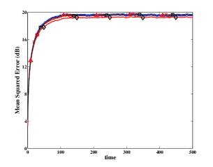
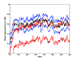
(a) $t\in[0,\;500],\;\delta=1,\;\mu_{t}\equiv 0.8$           (b) $t\in[80,\;500],\;\delta=1,\;\mu_{t}\equiv 0.8$

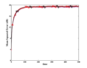
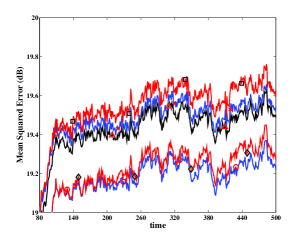
(c) $t\in[0,\;500],\;\delta=1,\;\mu_{t}\equiv 0.95$           (d) $t\in[80,\;500],\;\delta=1,\;\mu_{t}\equiv 0.95$

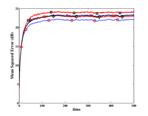
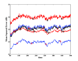
(e) $t\in[0,\;500],\;\delta=10,\;\mu_{t}\equiv 0.8$           (f) $t\in[80,\;500],\;\delta=10,\;\mu_{t}\equiv 0.8$

Figure 1: Empirical Mean Square Errors of Estimations. $-\!\!\!-\!\!\!\!\!\Box\!\!\!\!\!-\!\!\!-$: Kalman filter; $-\!\!\!-\!\!\!\!\!\Diamond\!\!\!\!\!-\!\!\!-$: estimator of [23]; $-\!\!\!-\!\!\!\!\!{\rm X}\!\!\!\!\!-\!\!\!-$: estimator of [27] ; $-\!\!\!-\!\!\!\!\!\triangle\!\!\!\!\!-\!\!\!-$: estimator of [16]; $-\!\!\!-\!\!\!\!\!{\scriptsize\bigcirc}\!\!\!\!\!-\!\!\!-$: estimator of this paper.

Kalman Filter, KFIO of [23], RSE of [27], the RSE with missing measurements (RSEMM) developed in [16], as well as the RSE developed in this paper (RSEIO), are utilized to estimate the plant states. When the Kalman filter, RSE of [27] and RSEMM are utilized, every received $y_{t}$ is regarded as a plant output measurement. Empirical MSE is used to measure estimation accuracy of these methods. More precisely, $5\times 10^{3}$ numerical experiments are performed with the temporal variable $t$ varies from $0$ to $5\times 10^{2}$. Let $x_{t}^{[j]}$ and $\hat{x}_{t}^{[j]}$ represent respectively the actual plant state and its estimate at the time instant $t$ in the $j$-th numerical experiment. Then, the empirical MSE of estimations at this time instant is defined as follows

$$\frac{1}{5\times 10^{3}}\sum_{j=1}^{5\times 10^{3}}[x_{t}^{[j]}-\hat{x}_{t}^{[j]}]^{T}[x_{t}^{[j]}-\hat{x}_{t}^{[j]}]$$

In Figure 1a, simulation results with $\delta=1$ is shown. This case is completely the same as that of [16]. To make the differences among these curves clear when the temporal variable $t$ takes a large value, in Figure 1b, they are re-plotted for the time interval $80\leq t\leq 5\times 10^{2}$. From these simulations, it becomes clear that when modelling errors fall into the interval $[-1,\;1]$, KFIO outperforms RSEIO. This is not a surprise, but only means that for this numerical example, estimation accuracy of the Kalman filter is not very sensitive to modelling errors, and in order to make a better trade-off between nominal performance and accuracy deteriorations, a greater value should be selected for the design parameter $\mu_{t}$ of RSEIO. As a matter of fact, actual computations show that if this design parameter is selected to be $0.95$, then, RSEIO will have a slightly higher estimation accuracy than KFIO. The corresponding results are given in Figures 1c and 1d.

To clarify necessities to take into account of modelling errors in state estimations, as well as influences of the design parameter $\mu_{t}$ on estimation accuracy, simulation results with $\delta=10$ and $\mu_{t}\equiv 0.8$ are also provided in Figures 1e and 1f. Results of these sub-figures clearly show that when the magnitude of modelling errors is large, sensitivity reduction for the innovation process of the Kalman filter is really very helpful in increasing its robustness against parametric modelling errors, and therefore improve its estimation accuracy. It is also clear from these simulation results that an appropriate selection of the estimator design parameter $\mu_{t}$ heavily depends on specific descriptions of modelling errors, such as their variation intervals, etc.

In all these computations, RSEIO has a better estimation accuracy than both RSE of [27] and RSEMM of [16]. This result may imply that information about random measurement droppings is more efficiently utilized by the estimation procedure of this paper, and the cost function $J(x_{t|t+1},\;w_{t|t+1})$ of Equation (5) is more physically reasonable than that adopted in [16] when information is contained in $y_{t+1}$ about whether or not it is a plant output measurement.

These simulation results also show that KFIO outperforms the traditional Kalman filter appreciably, but in comparison with RSE of [27], accuracy improvement by RSEMM is not very significant.

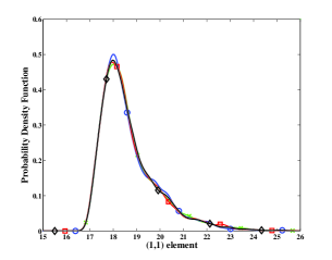
(a) the 1st row 1st column element                   (b) the 1st row 2nd column element

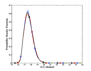
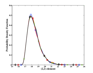
(c) the 2nd row 1st column element                   (d) the 2nd row 2nd column element

Figure 2: Empirical Probability Density Function for Elements of the Pseudo-Covariance Matrix at $t=500$. $-\!\!\!-\!\!\!\!\!{\rm X}\!\!\!\!\!-\!\!\!-$: $P_{0|0}=0.1I_{2}$; $-\!\!\!-\!\!\!\!\!{\scriptsize\bigcirc}\!\!\!\!\!-\!\!\!-$: $P_{0|0}=I_{2}$; $-\!\!\!-\!\!\!\!\!\Box\!\!\!\!\!-\!\!\!-$: $P_{0|0}=10I_{2}$; $-\!\!\!-\!\!\!\!\!\Diamond\!\!\!\!\!-\!\!\!-$: $P_{0|0}=100I_{2}$.

In Figure 2, empirical probability density function (EPDF) is shown for every element of the PCM $P_{t|t}$ at $t=5\times 10^{2}$ with 4 different initial $P_{0|0}$. In computing these EPDFs, $5\times 10^{3}$ independent numerical experiments have been performed for each situation and the Matlab file ksdensity.m is used with default parameters in estimating the EPDF. Moreover, the magnitude bound of modelling errors and the RSEIO design parameter are respectively selected as $\delta=10$ and $\mu_{t}\equiv 0.8$. From this figure, it is clear that although the initial $P_{0|0}$s are significantly distinct from each other, the EPDFs are very close for every element of the final $P_{500|500}$. This confirms the theoretical results on the convergence of the RESIO. On the other hand, it appears that the PDF of every element of the stationary PCM is a continuous function, which is greatly different from the conclusion about KFIO, in which it has been demonstrated in [13] that the stationary distribution has a fractured support. Moreover, the EPDFs of the non-diagonal elements are almost the same. This is due to the symmetry of the PCM.

It is worthwhile to point out that the comparisons of [16], in both its theoretical analyzes and its numerical simulations, are not appropriate, noting that in [25], a one-step recursive robust state predictor is derived, while the problem discussed in [16] is to robustly estimate plant state using current and past observations. In fact, from Figure 1, it is clear that estimation accuracy of RSEMM is even slightly worse than the traditional Kalman filter, in which neither parametric errors nor random measurement droppings are taken into account. However, it is declared in [16] that RSEMM is slightly better than the estimator of [25], while [25] claims its superiority over the traditional Kalman filter in prediction accuracies. These conclusions are apparently contradictory. Moreover, the numerical examples adopted in these two papers are completely different. In addition, time averaging is adopted in [25] for estimation accuracy evaluations, but [16] used ensemble averaging. These differences make the comparisons more unreasonable and the conclusions more confusing. Regretfully, these important things have been overlooked by this author.

V Concluding Remarks

In this paper, the sensitivity penalization based robust state estimation procedure is extended to situations in which plant output measurements may be randomly dropped due to communication failures. A new recursion formula has been derived for the PCM of estimation errors. Necessary and sufficient conditions have been established for the strict contractiveness of an iteration of this recursion. It has been proved that under some controllability and observability conditions, as well as some weak restrictions on the arrival probability of plant output measurements, the gain matrix of the developed RSE converges with probability one to a stationary distribution. Numerical simulations show that this RSE may outperform the well known Kalman filter in estimation accuracy.

While some progress have been made in robust state estimations with random measurement droppings, various important issues ask for further efforts. Among them, more general and less conservative conditions for the convergence of the obtained RSE, explicit expressions for the stationary distribution of the PCM, etc., seem essential in determining required capacity of a communication channel and selecting a suitable estimator design parameter.

Appendix: Proof of Some Technical Results

In order to prove the theoretical results of this paper, the following results are required, which are well known in matrix analysis and linear estimations, and can be straightforwardly proved through algebraic manipulations [11, 10].

Lemma A1. For arbitrary matrices $A,\;B,\;C,\;D$ with compatible dimensions, assume that all the involved matrix inverses exist. Then

$$\left[\begin{array}[]{cc}A&B\\ C&D\end{array}\right]=\left[\begin{array}[]{cc}I&0\\ CA^{-1}&I\end{array}\right]\left[\begin{array}[]{cc}A&0\\ 0&D-CA^{-1}B\end{array}\right]\left[\begin{array}[]{cc}I&A^{-1}B\\ 0&I\end{array}\right]$$ (a.9)

$$\hskip 56.9055pt=\left[\begin{array}[]{cc}I&BD^{-1}\\ 0&I\end{array}\right]\left[\begin{array}[]{cc}A-BD^{-1}C&0\\ 0&D\end{array}\right]\left[\begin{array}[]{cc}I&0\\ D^{-1}C&I\end{array}\right]$$ (a.16)

$$[A+CBD]^{-1}=A^{-1}-A^{-1}C[B^{-1}+DA^{-1}C]^{-1}DA^{-1}$$ (a.17)

$$A(I+BA)^{-1}=(I+AB)^{-1}A$$ (a.18)

Proof of Theorem 1: For brevity, define vectors $\alpha_{t}$ and $\alpha_{t0}$ respectively as $\alpha_{t}={\rm\bf col}\!\{x_{t|t+1},\;w_{t|t+1}\}$ and $\alpha_{t0}={\rm\bf col}\!\{\hat{x}_{t|t},\;0\}$. Moreover, define matrices $\bar{P}_{t|t}$, $\bar{Q}_{t}$, $\bar{B}_{t}(0)$ and $\bar{A}_{t}(0)$ respectively as

$$\bar{P}_{t|t}=(P_{t|t}^{-1}+\lambda_{t}\gamma_{t+1}S_{t}^{T}S_{t})^{-1},\hskip 14.22636pt\bar{Q}_{t}=\left[Q_{t}^{-1}+\lambda_{t}\gamma_{t+1}T_{t}^{T}(I+\lambda_{t}\gamma_{t+1}S_{t}P_{t|t}S_{t}^{T})T_{t}\right]^{-1}$$

$$\bar{B}_{t}(0)=B_{t}(0)-\lambda_{t}\gamma_{t+1}A_{t}(0)\bar{P}_{t|t}S_{t}^{T}T_{t},\hskip 7.11317pt\bar{A}_{t}(0)=[A_{t}(0)-\lambda_{t}\gamma_{t+1}\bar{B}_{t}(0)\bar{Q}_{t}T_{t}^{T}S_{t}][I-\lambda_{t}\gamma_{t+1}\bar{P}_{t|t}S_{t}^{T}S_{t}]$$

Furthermore, abbreviate $A_{t}(0)$, $\bar{A}_{t}(0)$, $B_{t}(0)$, $\bar{B}_{t}(0)$ and $C_{t}(0)$ respectively as $A_{t}$, $\bar{A}_{t}$, $B_{t}$, $\bar{B}_{t}$ and $C_{t}$. Note that for every $k\in\{1,2,\cdots,n\}$, we have

$$\frac{\partial e_{t}(\varepsilon_{t},\;\varepsilon_{t+1})}{\partial\varepsilon_{t,k}}=-C_{t+1}(\varepsilon_{t+1})\frac{\partial A_{t}(\varepsilon_{t})}{\partial\varepsilon_{t,k}}x_{t|t+1}-C_{t+1}(\varepsilon_{t+1})\frac{\partial B_{t}(\varepsilon_{t})}{\partial\varepsilon_{t,k}}w_{t|t+1}$$ (a.19)

$$\frac{\partial e_{t}(\varepsilon_{t},\;\varepsilon_{t+1})}{\partial\varepsilon_{t+1,k}}=-\frac{\partial C_{t+1}(\varepsilon_{t+1})}{\partial\varepsilon_{t+1,k}}A_{t}(\varepsilon_{t})x_{t|t+1}-\frac{\partial C_{t+1}(\varepsilon_{t+1})}{\partial\varepsilon_{t+1,k}}B_{t}(\varepsilon_{t})w_{t|t+1}$$ (a.20)

Then, from the definition of the cost function $J(x_{t|t+1},w_{t|t+1})$, it can be straightforwardly proved that

$$J(\alpha_{t})\!=\!\frac{\mu_{t}}{2}\!\left\{\!\!(\star)^{T}\!\!{\rm\bf diag}\!\left\{\!P_{t|t}^{-1}\!,\;\!Q_{t}^{-1}\!\right\}\!\!(\alpha_{t}\!\!-\!\!\alpha_{t0})\!\!+\!\!\gamma_{t\!+\!1}(\star)^{T}R_{t\!+\!1}^{-1}(C_{t\!+\!1}[A_{t}\;B_{t}]\alpha_{t}\!\!-\!\!y_{t+1})\!\!+\!\!\lambda_{t}\gamma_{t\!+\!1}(\star)^{T}([S_{t}\;T_{t}]\alpha_{t})\!\!\right\}$$ (a.21)

Therefore,

$$\frac{\partial J(\alpha_{t})}{\partial\alpha_{t}}\!\!\!\! = \!\!\!\!\mu_{t}\!\left\{\!\!{\rm\bf diag}\left\{\!P_{t|t}^{-1},\;Q_{t}^{-1}\!\right\}\!\!(\alpha_{t}\!-\!\alpha_{t0})\!+\!\gamma_{t+1}(C_{t+1}[A_{t}\;B_{t}])^{T}R_{t+1}^{-1}(C_{t+1}[A_{t}\;B_{t}]\alpha_{t}\!-\!y_{t+1})\!+\!\right.$$ (a.22)

$$\hskip 241.84842pt\left.\lambda_{t}\gamma_{t+1}[S_{t}\;T_{t}]^{T}[S_{t}\;T_{t}]\alpha_{t}\!\!\right\}$$

$$= \!\!\!\!\mu_{t}\!\left\{\!\!\left(\!\!{\rm\bf diag}\!\left\{\!P_{t|t}^{-1}\!,\;\!Q_{t}^{-1}\!\right\}+\lambda_{t}\gamma_{t\!+\!1}\![S_{t}\;T_{t}]^{T}[S_{t}\;T_{t}]\!+\!\gamma_{t\!+\!1}[A_{t}\;B_{t}]^{T}C_{t\!+\!1}^{T}R_{t\!+\!1}^{-1}C_{t\!+\!1}[A_{t}\;B_{t}]\!\!\right)\!\!\alpha_{t}\!-\right.$$

$$\hskip 113.81102pt\left.{\rm\bf diag}\left\{\!P_{t|t}^{-1},\;Q_{t}^{-1}\!\right\}\alpha_{t0}-\gamma_{t+1}[A_{t}\;B_{t}]^{T}C_{t+1}^{T}R_{t+1}^{-1}y_{t+1}\right\}$$

Note that $J(\alpha_{t})$ is a convex function and $\mu_{t}\neq 0$. It is obvious that the optimal $\alpha_{t}$, denote it by $\hat{\alpha}_{t}$, which minimizes $J(\alpha_{t})$, is given by its first derivative condition. That is,

$$\hat{\alpha}_{t}\!\! = \!\!\left\{\!\!{\rm\bf diag}\left\{\!P_{t|t}^{-1},\;\!Q_{t}^{-1}\!\right\}+\lambda_{t}\gamma_{t+1}[S_{t}\;T_{t}]^{T}[S_{t}\;T_{t}]+\gamma_{t+1}[A_{t}\;B_{t}]^{T}C_{t+1}^{T}R_{t+1}^{-1}C_{t+1}[A_{t}\;B_{t}]\!\!\right\}^{-1}\times$$ (a.23)

$$\hskip 85.35826pt\left\{{\rm\bf diag}\left\{\!P_{t|t}^{-1},\;\!Q_{t}^{-1}\!\right\}\alpha_{t0}+\gamma_{t+1}[A_{t}\;B_{t}]^{T}C_{t+1}^{T}R_{t+1}^{-1}y_{t+1}\right\}$$

On the other hand, direct algebraic manipulations show that

$$T_{t}^{T}T_{t}-\lambda_{t}\gamma_{t+1}T_{t}^{T}S_{t}[P_{t|t}^{-1}+\lambda_{t}\gamma_{t+1}S_{t}^{T}S_{t}]^{-1}S_{t}^{T}T_{t}=T_{t}^{T}[I+\lambda_{t}\gamma_{t+1}S_{t}P_{t|t}S_{t}^{T}]^{-1}T_{t}$$ (a.24)

Then, from Lemma A1 and the definitions of the matrices $\bar{P}_{t|t}$ and $\bar{Q}_{t}$, the following relation can be immediately obtained,

$${\rm\bf diag}\left\{\!P_{t|t}^{-1},\;\!Q_{t}^{-1}\!\right\}\!+\!\lambda_{t}\gamma_{t\!+\!1}[S_{t}\;T_{t}]^{T}[S_{t}\;T_{t}]\!\!=\!\!\left[\!\!\begin{array}[]{cc}I&0\\ \lambda_{t}\gamma_{t\!+\!1}T_{t}^{T}S_{t}\bar{P}_{t|t}&I\end{array}\!\!\right]\!\left[\!\!\begin{array}[]{cc}\bar{P}_{t|t}^{-1}&0\\ 0&\bar{Q}_{t}^{-1}\end{array}\!\!\right]\left[\!\!\begin{array}[]{cc}I&\lambda_{t}\gamma_{t\!+\!1}\bar{P}_{t|t}S_{t}^{T}T_{t}\\ 0&I\end{array}\!\!\right]$$ (a.25)

Substitute this relation into Equation (a.23), it can be further proved that

$$\hat{\alpha}_{t}\!\! = \!\!\left\{\!\!\left[\begin{array}[]{cc}I&0\\ \lambda_{t}\gamma_{t+1}T_{t}^{T}S_{t}\bar{P}_{t|t}&I\end{array}\right]\left[\begin{array}[]{cc}\bar{P}_{t|t}^{-1}&0\\ 0&\bar{Q}_{t}^{-1}\end{array}\right]\left[\begin{array}[]{cc}I&\lambda_{t}\gamma_{t+1}\bar{P}_{t|t}S_{t}^{T}T_{t}\\ 0&I\end{array}\right]+\right.$$

$$\hskip 14.22636pt\left.\gamma_{t+1}[A_{t}\;B_{t}]^{T}C_{t+1}^{T}R_{t+1}^{-1}C_{t+1}[A_{t}\;B_{t}]\!\!\right\}^{-1}\left\{{\rm\bf diag}\left\{\!P_{t|t}^{-1},\;Q_{t}^{-1}\!\right\}\alpha_{t0}+\gamma_{t+1}[A_{t}\;B_{t}]^{T}C_{t+1}^{T}R_{t+1}^{-1}y_{t+1}\right\}$$

$$= \!\!\left[\begin{array}[]{cc}I&-\lambda_{t}\gamma_{t+1}\bar{P}_{t|t}S_{t}^{T}T_{t}\\ 0&I\end{array}\right]\left\{\!\!\left[\begin{array}[]{cc}\bar{P}_{t|t}^{-1}&0\\ 0&\bar{Q}_{t}^{-1}\end{array}\right]+\gamma_{t+1}[A_{t}\;\bar{B}_{t}]^{T}C_{t+1}^{T}R_{t+1}^{-1}C_{t+1}[A_{t}\;\bar{B}_{t}]\!\!\right\}^{-1}\times$$ (a.38)

$$\hskip 85.35826pt\left[{\rm\bf col}\!\!\left\{I,\;\!-\lambda_{t}\gamma_{t+1}T_{t}^{T}S_{t}\bar{P}_{t|t}\right\}P_{t|t}^{-1}\hat{x}_{t|t}+\gamma_{t+1}[A_{t}\;\bar{B}_{t}]^{T}C_{t+1}^{T}R_{t+1}^{-1}y_{t+1}\right]$$

Hence,

$$\hat{x}_{t+1|t+1}\!\! = \!\![A_{t}\;B_{t}]\hat{\alpha}_{t}$$ (a.39)

$$= \!\![A_{t}\;\bar{B}_{t}]\left\{\!\!{\rm\bf diag}\left\{\!\bar{P}_{t|t}^{-1},\;\bar{Q}_{t}^{-1}\right\}+\gamma_{t+1}[A_{t}\;\bar{B}_{t}]^{T}C_{t+1}^{T}R_{t+1}^{-1}C_{t+1}[A_{t}\;\bar{B}_{t}]\!\!\right\}^{-1}\times$$

$$\hskip 85.35826pt\left\{{\rm\bf col}\!\!\left\{I,\;\!-\lambda_{t}\gamma_{t+1}T_{t}^{T}S_{t}\bar{P}_{t|t}\right\}P_{t|t}^{-1}\hat{x}_{t|t}+\gamma_{t+1}[A_{t}\;\bar{B}_{t}]^{T}C_{t+1}^{T}R_{t+1}^{-1}y_{t+1}\right\}$$

$$= \!\![A_{t}\;\bar{B}_{t}]\left\{\!\!I+\gamma_{t+1}{\rm\bf diag}\left\{\!\bar{P}_{t|t},\;\bar{Q}_{t}\right\}[A_{t}\;\bar{B}_{t}]^{T}C_{t+1}^{T}R_{t+1}^{-1}C_{t+1}[A_{t}\;\bar{B}_{t}]\!\right\}^{-1}{\rm\bf diag}\left\{\!\bar{P}_{t|t},\;\bar{Q}_{t}\!\right\}\times$$

$$\hskip 85.35826pt\left\{{\rm\bf col}\!\!\left\{I,\;\!-\lambda_{t}\gamma_{t+1}T_{t}^{T}S_{t}\bar{P}_{t|t}\right\}P_{t|t}^{-1}\hat{x}_{t|t}+\gamma_{t+1}[A_{t}\;\bar{B}_{t}]^{T}C_{t+1}^{T}R_{t+1}^{-1}y_{t+1}\right\}$$

$$= \!\!\left\{\!\!I+\gamma_{t+1}[A_{t}\;\bar{B}_{t}]{\rm\bf diag}\left\{\!\bar{P}_{t|t},\;\bar{Q}_{t}\!\right\}[A_{t}\;\bar{B}_{t}]^{T}C_{t+1}^{T}R_{t+1}^{-1}C_{t+1}\!\!\right\}^{-1}[A_{t}\;\bar{B}_{t}]{\rm\bf diag}\left\{\!\bar{P}_{t|t},\;\bar{Q}_{t}\!\right\}\times$$

$$\hskip 85.35826pt\left\{{\rm\bf col}\!\!\left\{I,\;\!-\lambda_{t}\gamma_{t+1}T_{t}^{T}S_{t}\bar{P}_{t|t}\right\}P_{t|t}^{-1}\hat{x}_{t|t}+\gamma_{t+1}[A_{t}\;\bar{B}_{t}]^{T}C_{t+1}^{T}R_{t+1}^{-1}y_{t+1}\right\}$$

$$= \!\!\left[I+\gamma_{t+1}P_{t+1|t}C_{t+1}^{T}R_{t+1}^{-1}C_{t+1}\right]^{-1}\left\{\bar{A}_{t}\hat{x}_{t|t}+\gamma_{t+1}P_{t+1|t}C_{t+1}^{T}R_{t+1}^{-1}y_{t+1}\right\}$$

in which $P_{t+1|t}=A_{t}\bar{P}_{t|t}A_{t}^{T}+\bar{B}_{t}\bar{Q}_{t}\bar{B}_{t}^{T}$. In the derivation of the last equality of the above equation, the relation $\bar{P}_{t|t}P_{t|t}^{-1}=I-\lambda_{t}\gamma_{t+1}\bar{P}_{t|t}S_{t}^{T}S_{t}$ has been utilized, which is a direct result of the definition of the matrix $\bar{P}_{t|t}$.

Therefore,

$$\hat{x}_{t+1|t+1}\!\! = \!\!\bar{A}_{t}\hat{x}_{t|t}+\gamma_{t+1}\left[I+\gamma_{t+1}P_{t+1|t}C_{t+1}^{T}R_{t+1}^{-1}C_{t+1}\right]^{-1}P_{t+1|t}C_{t+1}^{T}R_{t+1}^{-1}y_{t+1}$$ (a.40)

$$\hskip 56.9055pt-\gamma_{t+1}\left[I+\gamma_{t+1}P_{t+1|t}C_{t+1}^{T}R_{t+1}^{-1}C_{t+1}\right]^{-1}P_{t+1|t}C_{t+1}^{T}R_{t+1}^{-1}C_{t+1}\bar{A}_{t}\hat{x}_{t|t}$$

$$= \!\!\bar{A}_{t}\hat{x}_{t|t}+\gamma_{t+1}\left[P_{t+1|t}^{-1}+\gamma_{t+1}C_{t+1}^{T}R_{t+1}^{-1}C_{t+1}\right]^{-1}C_{t+1}^{T}R_{t+1}^{-1}\left\{y_{t+1}-C_{t+1}\bar{A}_{t}\hat{x}_{t|t}\right\}$$

Comparing this recursive formula for $\hat{x}_{t+1|t+1}$ with that of the Kalman filter given in [12, 11, 22], it is clear that the matrix $[P_{t+1|t}^{-1}+\gamma_{t+1}C_{t+1}^{T}R_{t+1}^{-1}C_{t+1}]^{-1}$ plays the same role as that of the covariance matrix of estimation errors in Kalman filtering. It is therefore reasonable to denote it by $P_{t+1|t+1}$. The proof can now be completed by noting that if $\gamma_{t+1}=0$, then $\bar{A}_{t}=A_{t}(0)$, $\bar{B}_{t}=B_{t}(0)$, $\bar{P}_{t|t}=P_{t|t}$ and $\bar{Q}_{t}=Q_{t}$, as well as that if $\gamma_{t+1}=1$, then $\bar{A}_{t}=\hat{A}_{t}(0)$, $\bar{B}_{t}=\hat{B}_{t}(0)$, $\bar{P}_{t|t}=\hat{P}_{t|t}$ and $\bar{Q}_{t}=\hat{Q}_{t}$. $\Diamond$

Proof of Theorem 2: To simplify mathematical expressions, in this proof, $A_{t}(0)$, $B_{t}(0)$ and $C_{t+1}(0)$ are again respectively abbreviated to be $A_{t}$, $B_{t}$ and $C_{t+1}$. From the proof of Theorem 1, it is clear that when $\gamma_{t+1}=1$,

$$\hat{x}_{t+1|t+1}\!\! = \!\![A_{t}\;B_{t}]\left\{\!\!{\rm\bf diag}\left\{\!P_{t|t}^{-1},\;\!Q_{t}^{-1}\!\right\}+\lambda_{t}[S_{t}\;T_{t}]^{T}[S_{t}\;T_{t}]+[A_{t}\;B_{t}]^{T}C_{t+1}^{T}R_{t+1}^{-1}C_{t+1}[A_{t}\;B_{t}]\!\!\right\}^{-1}\times$$ (a.41)

$$\hskip 85.35826pt\left\{{\rm\bf diag}\!\!\left\{\!P_{t|t}^{-1},\;Q_{t}^{-1}\!\right\}\!{\rm\bf col}\!\!\left\{\hat{x}_{t|t},\;0\right\}+[A_{t}\;B_{t}]^{T}C_{t+1}^{T}R_{t+1}^{-1}y_{t+1}\right\}$$

Moreover, Theorem 1 also declares that under such a situation,

$$\hat{x}_{t+1|t+1}=\hat{A}_{t}\hat{x}_{t|t}+P_{t+1|t+1}C_{t+1}^{T}R_{t+1}^{-1}[y_{t+1}-C_{t+1}\hat{A}_{t}\hat{x}_{t|t}]$$ (a.42)

As Equations (a.41) and (a.42) are just two different expressions for the same state estimate $\hat{x}_{t+1|t+1}$, the coefficient matrices respectively for $\hat{x}_{t|t}$ and $y_{t+1}$ should be equal to each other. A comparison of the coefficient matrices of $y_{t+1}$ show that

$$P_{t+1|t+1}=[A_{t}\;B_{t}]\left\{\!\!{\rm\bf diag}\left\{\!P_{t|t}^{-1},\;\!Q_{t}^{-1}\!\right\}+\lambda_{t}[S_{t}\;T_{t}]^{T}[S_{t}\;T_{t}]+[A_{t}\;B_{t}]^{T}C_{t+1}^{T}R_{t+1}^{-1}C_{t+1}[A_{t}\;B_{t}]\!\!\right\}^{\!-1}\!\!\!\!\![A_{t}\;B_{t}]^{T}$$ (a.43)

On the other hand, direct algebraic operations show that

$$\lambda_{t}S_{t}^{T}S_{t}-\lambda_{t}^{2}S_{t}^{T}T_{t}[Q_{t}^{-1}+\lambda_{t}T_{t}^{T}T_{t}]^{-1}T_{t}^{T}S_{t} = \lambda_{t}S_{t}^{T}\left\{I-\lambda_{t}T_{t}[I+\lambda_{t}Q_{t}T_{t}^{T}T_{t}]^{-1}Q_{t}T_{t}^{T}\right\}S_{t}$$ (a.44)

$$= \lambda_{t}S_{t}^{T}[I+\lambda_{t}T_{t}Q_{t}T_{t}^{T}]^{-1}S_{t}$$

$$= \tilde{S}_{t}^{T}\tilde{S}_{t}$$

Then, from Lemma A1 and the definition of $\check{Q}_{t}$, the following relation can be immediately obtained,

$${\rm\bf diag}\left\{\!P_{t|t}^{-1},\;\!Q_{t}^{-1}\!\right\}\!+\!\lambda_{t}[S_{t}\;T_{t}]^{T}[S_{t}\;T_{t}]\!=\!\left[\!\!\begin{array}[]{cc}I&\lambda_{t}S_{t}^{T}T_{t}\check{Q}_{t}\\ 0&I\end{array}\!\!\right]\!\left[\!\!\begin{array}[]{cc}P_{t|t}^{-1}+\tilde{S}_{t}^{T}\tilde{S}_{t}&0\\ 0&\check{Q}_{t}^{-1}\end{array}\!\!\right]\!\left[\!\!\begin{array}[]{cc}I&0\\ \lambda_{t}\check{Q}_{t}T_{t}^{T}S_{t}&I\end{array}\!\!\right]$$ (a.45)

Substitute Equation (a.45) into Equation (a.43), we have

$$P_{t+1|t+1}\!\! = \!\!\!\!\left(\!\![A_{t}\;B_{t}]\left[\!\!\begin{array}[]{cc}I&0\\ \lambda_{t}\check{Q}_{t}T_{t}^{T}S_{t}&I\end{array}\!\!\right]^{\!\!-1}\!\right)\!\!\left\{\!\!\left[\!\!\begin{array}[]{cc}P_{t|t}^{-1}\!+\!\tilde{S}_{t}^{T}\tilde{S}_{t}&0\\ 0&\check{Q}_{t}^{-1}\end{array}\!\!\right]\!+\!\left(\!\![A_{t}\;B_{t}]\left[\begin{array}[]{cc}I&0\\ \lambda_{t}\check{Q}_{t}T_{t}^{T}S_{t}&I\end{array}\right]^{\!\!-1}\!\right)^{T}\right.\!\!\!\!\times$$

$$\hskip 14.22636pt\left.C_{t+1}^{T}R_{t+1}^{-1}C_{t+1}\left([A_{t}\;B_{t}]\!\!\left[\!\!\begin{array}[]{cc}I&0\\ \lambda_{t}\check{Q}_{t}T_{t}^{T}S_{t}&I\end{array}\!\!\right]^{-1}\!\right)\!\!\right\}^{\!-1}\!\!\!\!\left(\!\![A_{t}\;B_{t}]\!\!\left[\!\!\begin{array}[]{cc}I&0\\ \lambda_{t}\check{Q}_{t}T_{t}^{T}S_{t}&I\end{array}\!\!\right]^{-1}\!\right)^{T}$$

$$= \!\!\!\![\check{A}_{t}\;B_{t}]\!\!\left\{\!\!{\rm\bf diag}\left\{\!P_{t|t}^{-1}\!+\!\tilde{S}_{t}^{T}\tilde{S}_{t},\;\check{Q}_{t}^{-1}\!\right\}\!+\![\check{A}_{t}\;B_{t}]^{T}C_{t+1}^{T}R_{t+1}^{-1}C_{t+1}[\check{A}_{t}\;B_{t}]\!\!\right\}^{-1}\!\![\check{A}_{t}\;B_{t}]^{T}$$

$$= \!\!\!\!\left\{\!\!I\!+\![\check{A}_{t}\;B_{t}]{\rm\bf diag}\left\{\!(P_{t|t}^{-1}\!+\!\tilde{S}_{t}^{T}\tilde{S}_{t})^{-1},\;\check{Q}_{t}\!\right\}\!\![\check{A}_{t}\;B_{t}]^{T}C_{t+1}^{T}R_{t+1}^{-1}C_{t+1}\!\!\right\}^{\!\!-1}\!\!\!\!\times$$

$$\hskip 170.71652pt[\check{A}_{t}\;B_{t}]{\rm\bf diag}\left\{\!(P_{t|t}^{-1}\!+\!\tilde{S}_{t}^{T}\tilde{S}_{t})^{-1},\;\check{Q}_{t}\!\right\}\!\![\check{A}_{t}\;B_{t}]^{T}$$

$$= \!\!\!\!\left\{\left[\check{A}_{t}(P_{t|t}^{-1}\!+\!\tilde{S}_{t}^{T}\tilde{S}_{t})^{-1}\check{A}^{T}_{t}+B_{t}\check{Q}_{t}B_{t}^{T}\right]^{-1}+C_{t+1}^{T}R_{t+1}C_{t+1}\right\}^{-1}$$ (a.58)

When $\check{A}_{t}$ is invertible, from the definition of the matrix $\tilde{B}_{t}$, we have that

$$\check{A}_{t}(P_{t|t}^{-1}\!+\!\tilde{S}_{t}^{T}\tilde{S}_{t})^{-1}\check{A}^{T}_{t}+B_{t}\check{Q}_{t}B_{t}^{T}=\check{A}_{t}\left\{(P_{t|t}^{-1}\!+\!\tilde{S}_{t}^{T}\tilde{S}_{t})^{-1}+\tilde{B}_{t}\check{Q}_{t}\tilde{B}_{t}^{T}\right\}\check{A}^{T}_{t}$$ (a.59)

Note that

$$\left\{(P_{t|t}^{-1}\!+\!\tilde{S}_{t}^{T}\tilde{S}_{t})^{-1}+\tilde{B}_{t}\check{Q}_{t}\tilde{B}_{t}^{T}\right\}^{-1}$$ (a.60)

$$= \!\!\!\!\left\{I+(P_{t|t}^{-1}\!+\!\tilde{S}_{t}^{T}\tilde{S}_{t})\tilde{B}_{t}\check{Q}_{t}\tilde{B}_{t}^{T}\right\}^{-1}(P_{t|t}^{-1}\!+\!\tilde{S}_{t}^{T}\tilde{S}_{t})$$

$$= \!\!\!\!\left\{\tilde{B}_{t}\check{Q}_{t}\tilde{B}_{t}^{T}+P_{t|t}(I+\tilde{S}_{t}^{T}\tilde{S}_{t}\tilde{B}_{t}\check{Q}_{t}\tilde{B}_{t}^{T})\right\}^{-1}(I+P_{t|t}\tilde{S}_{t}^{T}\tilde{S}_{t})$$

$$= \!\!\!\!\left\{\tilde{B}_{t}\check{Q}_{t}\tilde{B}_{t}^{T}+P_{t|t}(I+\tilde{S}_{t}^{T}\tilde{S}_{t}\tilde{B}_{t}\check{Q}_{t}\tilde{B}_{t}^{T})\right\}^{-1}\left\{I+\left[\tilde{B}_{t}\check{Q}_{t}\tilde{B}_{t}^{T}+P_{t|t}(I+\tilde{S}_{t}^{T}\tilde{S}_{t}\tilde{B}_{t}\check{Q}_{t}\tilde{B}_{t}^{T})\right](I+\right.$$

$$\hskip 113.81102pt\left.\tilde{S}_{t}^{T}\tilde{S}_{t}\tilde{B}_{t}\check{Q}_{t}\tilde{B}_{t}^{T})^{-1}\tilde{S}_{t}^{T}\tilde{S}_{t}-\tilde{B}_{t}\check{Q}_{t}\tilde{B}_{t}^{T}(I+\tilde{S}_{t}^{T}\tilde{S}_{t}\tilde{B}_{t}\check{Q}_{t}\tilde{B}_{t}^{T})^{-1}\tilde{S}_{t}^{T}\tilde{S}_{t}\right\}$$

$$= \!\!\!\!\tilde{S}_{t}^{T}(I+\tilde{S}_{t}\tilde{B}_{t}\check{Q}_{t}\tilde{B}_{t}^{T}\tilde{S}_{t}^{T})^{-1}\tilde{S}_{t}+\left\{\tilde{B}_{t}(\check{Q}_{t}+\check{Q}_{t}\tilde{B}_{t}^{T}\tilde{S}_{t}^{T}\tilde{S}_{t}\tilde{B}_{t}\check{Q}_{t})\tilde{B}_{t}^{T}+(I+\tilde{B}_{t}\check{Q}_{t}\tilde{B}_{t}^{T}\tilde{S}_{t}^{T}\tilde{S}_{t})P_{t|t}\!\times\right.$$

$$\hskip 227.62204pt\left.(I+\tilde{B}_{t}\check{Q}_{t}\tilde{B}_{t}^{T}\tilde{S}_{t}^{T}\tilde{S}_{t})^{T}\right\}^{-1}$$

Substitute Equations (a.59) and (a.60) into Equation (a.58), the following recursive expression for $P_{t+1|t+1}$ is obtained for situations when $\check{A}_{t}$ is invertible,

$$P_{t+1|t+1}^{-1}\!\!\!\! = \!\!\!\!\check{A}_{t}^{-T}\left[(P_{t|t}^{-1}\!+\!\tilde{S}_{t}^{T}\tilde{S}_{t})^{-1}+\tilde{B}_{t}\check{Q}_{t}\tilde{B}_{t}^{T}\right]^{-1}\check{A}_{t}^{-1}+C_{t+1}^{T}R_{t+1}C_{t+1}$$ (a.61)

$$= \!\!\!\!\check{A}_{t}^{-T}\!\!\left\{\!\!\tilde{B}_{t}(\check{Q}_{t}\!+\!\check{Q}_{t}\tilde{B}_{t}^{T}\tilde{S}_{t}^{T}\tilde{S}_{t}\tilde{B}_{t}\check{Q}_{t})\tilde{B}_{t}^{T}\!+\!(I\!+\!\tilde{B}_{t}\check{Q}_{t}\tilde{B}_{t}^{T}\tilde{S}_{t}^{T}\tilde{S}_{t})P_{t|t}(I\!+\!\tilde{B}_{t}\check{Q}_{t}\tilde{B}_{t}^{T}\tilde{S}_{t}^{T}\tilde{S}_{t})^{T}\!\right\}^{\!-1}\!\!\check{A}_{t}^{\!-1}\!+$$

$$\hskip 113.81102pt\check{A}_{t}^{-T}\tilde{S}_{t}^{T}(I+\tilde{S}_{t}\tilde{B}_{t}\check{Q}_{t}\tilde{B}_{t}^{T}\tilde{S}_{t}^{T})^{-1}\tilde{S}_{t}\check{A}_{t}^{-1}+C_{t+1}^{T}R_{t+1}C_{t+1}$$

$$= \!\!\!\!\left\{\!\!B_{t}(\check{Q}_{t}\!+\!\check{Q}_{t}\tilde{B}_{t}^{T}\tilde{S}_{t}^{T}\tilde{S}_{t}\tilde{B}_{t}\check{Q}_{t})B_{t}^{T}\!+\!(\check{A}_{t}\!+\!B_{t}\check{Q}_{t}\tilde{B}_{t}^{T}\tilde{S}_{t}^{T}\tilde{S}_{t})P_{t|t}(\check{A}_{t}\!+\!B_{t}\check{Q}_{t}\tilde{B}_{t}^{T}\tilde{S}_{t}^{T}\tilde{S}_{t})^{T}\!\right\}^{\!-1}\!\!\!+$$

$$\hskip 113.81102pt(\tilde{S}_{t}\check{A}_{t}^{-1})^{T}(I+\tilde{S}_{t}\tilde{B}_{t}\check{Q}_{t}\tilde{B}_{t}^{T}\tilde{S}_{t}^{T})^{-1}(\tilde{S}_{t}\check{A}_{t}^{-1})+C_{t+1}^{T}R_{t+1}C_{t+1}$$

$$= \!\!\!\![\tilde{A}_{t}P_{t|t}\tilde{A}_{t}^{T}+B_{t}\tilde{Q}_{t}B_{t}^{T}]^{-1}+\tilde{C}_{t+1}^{T}\tilde{R}_{t+1}^{-1}\tilde{C}_{t+1}$$

This completes the proof. $\Diamond$

Proof of Theorem 3: Define matrix $G_{o}$ as

$$G_{o}=\Phi_{N,11}^{T}\Phi_{N,21}+\sum_{i=N-1}^{1}\left[\left(\prod_{k=N}^{i}\Phi_{k,11}^{T}\right)\Phi_{i,21}\left(\prod_{k=i+1}^{N}\Phi_{k,11}\right)\right]$$

Then, it can be claimed from Lemma 2 that $\prod_{t=1}^{N}\Phi_{t}\in{\cal H}_{l}$ if and only if ${\rm\bf D}_{et}\left\{G_{o}\right\}\neq 0$.

Assume that at the sampling instants $t_{1},\;t_{2},\;\cdots\,\;t_{p}$, with $1\leq t_{1}<t_{2}<\cdots<t_{p}\leq N$, $\gamma_{k}=1$; and at any other sampling instants between $1$ and $N$, $\gamma_{k}=0$. Define $t_{0}$ as $t_{0}=0$. Then, according to the definition of $\Phi_{t}$, the following relation is obtained,

$$G_{o}\!=\!\sum_{j=0}^{p}\!\left[\!\left(\!\prod_{k=t_{j}+1}^{N}\Phi_{k,11}\!\right)^{T}\!\Phi_{t_{j},11}^{T}\Phi_{t_{j},21}\!\left(\!\prod_{k=t_{j}+1}^{N}\Phi_{k,11}\!\right)\!\right]$$ (a.62)

in which $\prod_{k=q}^{N}\Phi_{k,11}$ is defined to be the identity matrix if $q>N$. This situation occurs when $t_{p}=N$.

Note that for every $t_{j}$ with $1\leq j\leq p$,

$$\Phi_{t_{j},11}^{T}\Phi_{t_{j},12}=A^{[1]T}H^{[1]T}H^{[1]}A^{[1]}=(H^{[1]}A^{[1]})^{T}(H^{[1]}A^{[1]})$$ (a.63)

Moreover,

$$\prod_{k=t_{j}+1}^{N}\Phi_{k,11} = \prod_{k=t_{j}+1}^{t_{j+1}-1}\Phi_{k,11}\times\Phi_{t_{j+1},11}\times\prod_{k=t_{j+1}+1}^{t_{j+2}-1}\Phi_{k,11}\times\Phi_{t_{j+2},11}\times\cdots\times\prod_{k=t_{p}+1}^{N}\Phi_{k,11}$$ (a.64)

$$= (A^{[2]})^{t_{j+1}-t_{j}-1}A^{[1]}(A^{[2]})^{t_{j+2}-t_{j+1}-1}A^{[1]}\cdots(A^{[2]})^{N-t_{p}}$$

$$= \left(\prod_{s=j}^{p-1}\left[(A^{[2]})^{t_{s+1}-t_{s}-1}A^{[1]}\right]\right)(A^{[2]})^{N-t_{p}}$$

Substitute Equations (a.63) and (a.64) into Equation (a.62), the following relation is obtained,

$$G_{o}\!\!\!\! = \!\!\!\!\sum_{j=0}^{p}\left\{\!\!\left[\star\right]^{T}(H^{[1]}A^{[1]})^{T}(H^{[1]}A^{[1]})\left[\!\!\left(\prod_{s=j}^{p-1}\left[(A^{[2]})^{t_{s+1}-t_{s}-1}A^{[1]}\right]\right)(A^{[2]})^{N-t_{p}}\right)\right\}$$ (a.69)

$$= \!\!\!\!\sum_{j=0}^{p}\left\{\!\!\left[\star\right]^{T}\left[H^{[1]}A^{[1]}\left(\prod_{s=j}^{p-1}\left[(A^{[2]})^{t_{s+1}-t_{s}-1}A^{[1]}\right]\right)(A^{[2]})^{N-t_{p}}\right)\right\}$$

$$= \!\!\!\!\left[\star\right]^{T}\left[\begin{array}[]{c}H^{[1]}(A^{[2]})^{N-t_{p}}\\ H^{[1]}A^{[1]}(A^{[2]})^{t_{p}-t_{p-1}-1}(A^{[2]})^{N-t_{p}}\\ \vdots\\ H^{[1]}\prod_{j=1}^{p}\left(A^{[1]}(A^{[2]})^{t_{j}-t_{j-1}-1}\right)(A^{[2]})^{N-t_{p}}\end{array}\right]$$

$$= \!\!\!\!(A^{[2]T})^{N-t_{p}}O_{b}^{T}O_{b}(A^{[2]})^{N-t_{p}}$$ (a.70)

Recall that the matrix $A^{[2]}$ is assumed invertible. It is obvious from the above equality that the satisfaction of the inequality ${\rm\bf D}_{et}\left\{G_{o}\right\}\neq 0$ is equivalent to that the matrix $O_{b}$ is of full column rank. This completes the proof. $\Diamond$

Proof of Theorem 4: From Lemma 2, it can be claimed that $\prod_{t=1}^{N}\Phi_{t}\in{\cal H}_{r}$ if and only if ${\rm\bf D}_{et}\left\{G_{c}\right\}\neq 0$, in which

$$G_{c}=\Phi_{1,12}\Phi_{1,11}^{T}+\sum_{i=2}^{N}\left[\left(\prod_{k=1}^{i-1}\Phi_{k,11}\right)\Phi_{i,12}\left(\prod_{k=i}^{1}\Phi_{k,11}^{T}\right)\right]$$

Similar to the proof of Theorem 3, assume that at the sampling instants $t_{1},\;t_{2},\;\cdots\,\;t_{p}$, with $1\leq t_{1}<t_{2}<\cdots<t_{p}\leq N$, $\gamma_{k}=1$; and at any other sampling instants between $1$ and $N$, $\gamma_{k}=0$. Moreover, $t_{0}$ is once again defined as $t_{0}=0$. Furthermore, define $t_{p+1}$ as $t_{p+1}=N+1$.

Define $\prod_{k=1}^{0}\Phi_{k,11}$ as the identity matrix. It can then be easily seen that,

$$G_{c}=\sum_{i=1}^{N}\left[\left(\prod_{k=1}^{i-1}\Phi_{k,11}\right)\Phi_{i,12}\Phi_{i,11}^{T}\left(\prod_{k=1}^{i-1}\Phi_{k,11}\right)^{T}\right]$$ (a.71)

When $i\in\{t_{1},\;t_{2},\;\cdots,\;t_{p}\}$, assume that $i=t_{j}$, $j=1,2,\cdots,p$. We have

$$\Phi_{i,12}\Phi_{i,11}^{T}\!\!\!\! = \!\!\!\!\left[G^{[1]}G^{[1]T}(A^{[1]})^{-T}\right]A^{[1]T}=G^{[1]}G^{[1]T}$$ (a.72)

$$\prod_{k=1}^{i-1}\Phi_{k,11}\!\!\!\! = \!\!\!\!\left(\prod_{k=1}^{t_{1}-1}\Phi_{k,11}\right)\Phi_{t_{1},11}\left(\prod_{k=t_{1}+1}^{t_{2}-1}\Phi_{k,11}\right)\Phi_{t_{2},11}\cdots\left(\prod_{k=t_{j-1}+1}^{t_{j}-1}\Phi_{k,11}\right)$$ (a.73)

$$= \!\!\!\!(A^{[2]})^{t_{1}-1}A^{[1]}(A^{[2]})^{t_{2}-t_{1}-1}A^{[1]}\cdots(A^{[2]})^{t_{j}-t_{j-1}-1}$$

$$= \!\!\!\!(A^{[2]})^{t_{1}-1}\prod_{s=1}^{j-1}\left[A^{[1]}(A^{[2]})^{t_{s+1}-t_{s}-1}\right]$$

When $i\not\in\{t_{1},\;t_{2},\;\cdots,\;t_{p}\}$, assume that $t_{j-1}<i<t_{j}$, $j=1,2,\cdots,p+1$. On the basis of Equation (a.73), we then have

$$\Phi_{i,12}\Phi_{i,11}^{T}\!\!\!\! = \!\!\!\!\left[G^{[2]}G^{[2]T}(A^{[2]})^{-T}\right]A^{[2]T}=G^{[2]}G^{[2]T}$$ (a.74)

$$\prod_{k=1}^{i-1}\Phi_{k,11}\!\!\!\! = \!\!\!\!\left(\prod_{k=1}^{t_{j-1}-1}\Phi_{k,11}\right)\Phi_{t_{j-1},11}\left(\prod_{k=t_{j-1}+1}^{i-1}\Phi_{k,11}\right)$$ (a.75)

$$= \!\!\!\!(A^{[2]})^{t_{1}-1}\left(\prod_{s=1}^{j-2}\left[A^{[1]}(A^{[2]})^{t_{s+1}-t_{s}-1}\right]\right)A^{[1]}(A^{[2]})^{i-t_{j-1}-1}$$

When $1\leq i<t_{1}$, direct algebraic manipulations show that

$$\Phi_{i,12}\Phi_{i,11}^{T}\!\!\!\! = \!\!\!\!\left[G^{[2]}G^{[2]T}(A^{[2]})^{-T}\right]A^{[2]T}=G^{[2]}G^{[2]T}$$ (a.76)

$$\prod_{k=1}^{i-1}\Phi_{k,11}\!\!\!\! = \!\!\!\!\prod_{k=1}^{i-1}A^{[2]}\!=\!\left(A^{[2]}\right)^{i-1}$$ (a.77)

Substitute these relations into Equation (a.71), the following equalities are obtained.

$$G_{c}\!\!\!\! = \!\!\!\!\sum_{i=1}^{t_{1}-1}\left[\left(\prod_{k=1}^{i-1}\Phi_{k,11}\right)\Phi_{i,12}\Phi_{i,11}^{T}\left(\star\right)^{T}\right]+\sum_{j=2}^{p+1}\left\{\left[\left(\prod_{k=1}^{t_{j-1}-1}\Phi_{k,11}\right)\Phi_{t_{j-1},12}\Phi_{t_{j-1},11}^{T}\left(\star\right)^{T}\right]+\right.$$ (a.78)

$$\hskip 170.71652pt\left.\sum_{i=t_{j-1}+1}^{t_{j}-1}\left[\left(\prod_{k=1}^{i-1}\Phi_{k,11}\right)\Phi_{i,12}\Phi_{i,11}^{T}\left(\star\right)^{T}\right]\right\}$$

$$= \!\!\!\!\sum_{i=0}^{t_{1}-2}\left[\left(A^{[2]}\right)^{i}G^{[2]}\right]\left[\star\right]^{T}+(A^{[2]})^{t_{1}-1}\sum_{j=2}^{p+1}\left\{\left(\prod_{s=1}^{j-1}\left[A^{[1]}(A^{[2]})^{t_{s+1}-t_{s}-1}\right]G^{[1]}\right)\left(\star\right)^{T}+\right.$$

$$\hskip 14.22636pt\left.\sum_{i=t_{j-1}+1}^{t_{j}-1}\left(A^{[1]}\prod_{s=1}^{j-2}\left[(A^{[2]})^{t_{s+1}-t_{s}-1}A^{[1]}\right](A^{[2]})^{i-t_{j-1}-1}G^{[2]}\right)\left(\star\right)^{T}\right\}(A^{[2]T})^{t_{1}-1}$$

$$= \!\!\!\!C_{o}C_{o}^{T}$$

Therefore, the inequality ${\rm\bf D}_{et}\left\{G_{c}\right\}\neq 0$ is satisfied, if and only if the matrix $C_{o}$ is of full row rank. This completes the proof. $\Diamond$

Proof of Lemma 3: When $\gamma_{k}|_{k=1}^{\infty}$ is white and has a Bernoulli distribution, we have

$${\rm\bf P}_{r}\left(\Gamma^{[N]}=S_{m}^{[N]}\right) = \prod_{k=N}^{1}{\rm\bf P}_{r}\left(\gamma_{k}=S_{m}^{[N]}(k)\right)$$ (a.79)

$$= \prod_{k=N}^{1}\bar{\gamma}^{S_{m}^{[N]}(k)}(1-\bar{\gamma})^{1-S_{m}^{[N]}(k)}$$

Hence,

$${\rm log}\!\left[{\rm\bf P}_{r}\left(\Gamma^{[N]}=S_{m}^{[N]}\right)\right] = \sum_{i=1}^{N}\left[S_{m}^{[N]}(k){\rm log}\!(\bar{\gamma})+(1-S_{m}^{[N]}(k)){\rm log}\!(1-\bar{\gamma})\right]$$ (a.80)

$$= {\rm log}(\bar{\gamma})\sum_{i=1}^{N}S_{m}^{[N]}(i)+{\rm log}(1-\bar{\gamma})\left(N-\sum_{i=1}^{N}S_{m}^{[N]}(i)\right)$$

When $\gamma_{k}|_{k=1}^{\infty}$ is a Markov chain,

$${\rm\bf P}_{r}\left(\Gamma^{[N]}=S_{m}^{[N]}\right)=\left\{\prod_{k=N}^{2}{\rm\bf P}_{r}\left(\left.\gamma_{k}=S_{m}^{[N]}(k)\right|\gamma_{k-1}=S_{m}^{[N]}(k-1)\right)\right\}{\rm\bf P}_{r}\left(\gamma_{1}=S_{m}^{[N]}(1)\right)$$ (a.81)

Note that

$${\rm\bf P}_{r}\left(\gamma_{1}=S_{m}^{[N]}(1)\right)=\left\{\begin{array}[]{ll}(1-\alpha){\rm\bf P}_{r}(\gamma_{0}=1)+\beta{\rm\bf P}_{r}(\gamma_{0}=0)&S_{m}^{[N]}(1)=0\\ \alpha{\rm\bf P}_{r}(\gamma_{0}=1)+(1-\beta){\rm\bf P}_{r}(\gamma_{0}=0)&S_{m}^{[N]}(1)=1\end{array}\right.$$ (a.82)

It can therefore be concluded from the assumption ${\rm\bf P}_{r}(\gamma_{0}=1)=\bar{\gamma}$ and the fact that ${\rm\bf P}_{r}(\gamma_{0}=0)+{\rm\bf P}_{r}(\gamma_{0}=1)\equiv 1$ that

$${\rm\bf P}_{r}\left(\gamma_{1}=S_{m}^{[N]}(1)\right) = [1-S_{m}^{[N]}(1)]\left[(1-\alpha){\rm\bf P}_{r}(\gamma_{0}=1)+\beta{\rm\bf P}_{r}(\gamma_{0}=0)\right]+$$ (a.83)

$$\hskip 28.45274ptS_{m}^{[N]}(1)\left[\alpha{\rm\bf P}_{r}(\gamma_{0}=1)+(1-\beta){\rm\bf P}_{r}(\gamma_{0}=0)\right]$$

$$= S_{m}^{[N]}(1)\!+\![1\!-\!2S_{m}^{[N]}(1)][\beta\!+\!\bar{\gamma}(1\!-\!\alpha\!-\!\beta)]$$

On the other hand, for an arbitrary $k\in\{2,\;3,\;\cdots,\;N\}$, it can be straightforwardly declared from the definition of a Markov chain and the assumption $0<\alpha,\;\beta<1$ that

$${\rm\bf P}_{r}\left(\left.\gamma_{k}=S_{m}^{[N]}(k)\right|\gamma_{k-1}=S_{m}^{[N]}(k-1)\right)$$

$$= \left\{\begin{array}[]{lll}\alpha,&&S_{m}^{[N]}(k)=1,\;S_{m}^{[N]}(k-1)=1\\ 1-\alpha,&&S_{m}^{[N]}(k)=1,\;S_{m}^{[N]}(k-1)=0\\ \beta,&&S_{m}^{[N]}(k)=0,\;S_{m}^{[N]}(k-1)=1\\ 1-\beta,&&S_{m}^{[N]}(k)=0,\;S_{m}^{[N]}(k-1)=0\end{array}\right.$$

$$= \alpha^{S_{m}^{[N]}(k)S_{m}^{[N]}(k-1)}(1-\alpha)^{(1-S_{m}^{[N]}(k))S_{m}^{[N]}(k-1)}(1-\beta)^{S_{m}^{[N]}(k)(1-S_{m}^{[N]}(k-1))}\beta^{(1-S_{m}^{[N]}(k))(1-S_{m}^{[N]}(k-1))}$$

$$= \beta\left(\frac{1-\alpha}{\beta}\right)^{S_{m}^{[N]}(k-1)}\left(\frac{1-\beta}{\beta}\right)^{S_{m}^{[N]}(k)}\left(\frac{\alpha\beta}{(1-\alpha)(1-\beta)}\right)^{S_{m}^{[N]}(k)S_{m}^{[N]}(k-1)}$$ (a.89)

Substitute Equations (a.83) and (a.89) into Equation (a.81), the following relation is obtained,

$${\rm log}\!\left[{\rm\bf P}_{r}\!\left(\!\Gamma^{[N]}\!=\!S_{m}^{[N]}\right)\!\right]\!\!\!\! = \!\!\!\!\sum_{k=N}^{2}{\rm log}\!\left[{\rm\bf P}_{r}\left(\left.\gamma_{k}=S_{m}^{[N]}(k)\right|\gamma_{k-1}=S_{m}^{[N]}(k-1)\right)\right]+{\rm log}\!\left[{\rm\bf P}_{r}\left(\gamma_{1}=S_{m}^{[N]}(1)\right)\right]$$ (a.90)

$$= \!\!\!\!\sum_{k=N}^{2}\left\{{\rm log}(\beta)+S_{m}^{[N]}(k-1){\rm log}\!\left(\frac{1-\alpha}{\beta}\right)+S_{m}^{[N]}(k){\rm log}\!\left(\frac{1-\beta}{\beta}\right)+\right.$$

$$\hskip 56.9055pt\left.S_{m}^{[N]}(k)S_{m}^{[N]}(k-1){\rm log}\!\left(\frac{\alpha\beta}{(1-\alpha)(1-\beta)}\right)\right\}+$$

$$\hskip 56.9055pt{\rm log}\!\left\{S_{m}^{[N]}(1)\!+\![1\!-\!2S_{m}^{[N]}(1)][\beta\!+\!\bar{\gamma}(1\!-\!\alpha\!-\!\beta)]\right\}$$

$$= \!\!\!\!(N\!-\!1){\rm log}(\beta)\!+\!{\rm log}\!\left(\!\frac{1\!-\!\alpha}{\beta}\!\right)\!\sum_{k=1}^{N-1}\!S_{m}^{[N]}(k)\!+\!{\rm log}\!\left(\!\frac{1}{\beta}\!-\!1\!\right)\!\sum_{k=2}^{N}S_{m}^{[N]}(k)\!+$$

$$\!\!\!\!\hskip 56.9055pt{\rm log}\!\left(\!\frac{\alpha\beta}{(1\!-\!\alpha)(1\!-\!\beta)}\!\right)\!\sum_{k=2}^{N}\!\left[\!S_{m}^{[N]}(k)S_{m}^{[N]}(k\!-\!1)\!\right]\!+$$

$$\!\!\!\!\hskip 56.9055pt{\rm log}\!\left\{\!S_{m}^{[N]}(1)\!+\![1\!-\!2S_{m}^{[N]}(1)][\beta\!+\!\bar{\gamma}(1\!-\!\alpha\!-\!\beta)]\!\right\}$$

This completes the proof. $\Diamond$

Proof of Theorem 5: Assume that there exist two positive integers $m_{1}$ and $m_{2}$ such that the matrix pairs $(A^{[1]}(A^{[2]})^{m_{1}},\;H^{[1]})$ and $((A^{[2]})^{m_{2}}A^{[1]},\;G^{[2]})$ are respectively observable and controllable. Then, the following two matrices $\bar{O}_{b}$ and $\bar{C}_{n}$ are respectively of full column rank and full row rank,

$$\bar{O}_{b}=\left[\begin{array}[]{c}H^{[1]}\\ H^{[1]}A^{[1]}(A^{[2]})^{m_{1}}\\ \vdots\\ H^{[1]}\left(A^{[1]}(A^{[2]})^{m_{1}}\right)^{n-1}\end{array}\right],\hskip 14.22636pt\bar{C}_{n}=\left[G^{[2]}\;\;(A^{[2]})^{m_{2}}A^{[1]}G^{[2]}\cdots\left((A^{[2]})^{m_{2}}A^{[1]}\right)^{n-1}G^{[2]}\right]$$

Define positive integers $N_{*}$ and $N$, as well as a finite binary sequence $R^{[N]}=\{R^{[N]}(t)|_{t=1}^{N}\}$, respectively as $N_{*}=(n-2)(m_{1}+1)+1$, $N=(n-2)(m_{1}+m_{2}+2)+2$, and

$$R^{[N]}(t)=\left\{\begin{array}[]{lll}0&t\in\left(1+(j-1)(m_{1}+1),\;1+j(m_{1}+1)\right)\\ 1&t=1+(j-1)(m_{1}+1)\\ 0&t=N_{*}+(j-1)(m_{2}+1)+1\\ 1&t\in\left(N_{*}+(j-1)(m_{2}+1)+1,\;N_{*}+j(m_{2}+1)+1\right)\end{array}\right.$$ (a.91)

in which $j=1,2,\cdots,n-1$. Then, it can be claimed from Theorems 3 and 4 that when the finite random sequence $\Gamma^{[N]}$ has the realization $R^{[N]}$, the corresponding matrices $\Phi_{R^{[N]}(t)}|_{t=1}^{N}$ simultaneously satisfy $\prod_{t=1}^{N_{*}}\Phi_{R^{[N]}(t)}\in{\cal H}_{l}$ and $\prod_{t=N_{*}+1}^{N}\Phi_{R^{[N]}(t)}\in{\cal H}_{r}$. Hence, according to Lemma 2, $\prod_{t=1}^{N}\Phi_{R^{[N]}(t)}=\prod_{t=1}^{N_{*}}\Phi_{R^{[N]}(t)}\prod_{t=N_{*}+1}^{N}\Phi_{R^{[N]}(t)}$ belongs to both ${\cal H}_{l}$ and ${\cal H}_{r}$, and therefore ${\cal H}_{lr}$. It can therefore be declared from Lemma 2 that with respect to this particular realization of $\gamma_{t}|_{t=1}^{N}$, the corresponding matrix valued function ${\rm\bf H}_{m}\left(\prod_{t=1}^{N}\Phi_{R^{[N]}(t)},\star\right)$, which is defined on the set of $n\times n$ dimensional positive definite matrices, is strictly contractive under the Riemannian distance defined in Equation (LABEL:eqn:10). This means that if during the time interval $[1,\;N]$, the random measurement dropping process $\gamma_{t}|_{t=1}^{\infty}$ has this particular realization, then, ${\rm\bf L}_{ip}\!\left({\rm\bf H}_{m}\!\left(\prod_{t=1}^{N}\Phi_{R^{[N]}(t)},\star\right)\!\right)$ $<1$. From Lemma 1, this inequality is further equivalent to

$${\rm\bf L}_{ip}\left({\rm\bf H}_{m}\left(\Phi_{R^{[N]}(1)},{\rm\bf H}_{m}\left(\Phi_{R^{[N]}(2)},\cdots,{\rm\bf H}_{m}\left(\Phi_{R^{[N]}(N)},\star\right)\cdots\right)\right)\right)<1$$ (a.92)

On the other hand, from the definition of the set ${\cal S}^{[N]}$, it is obvious that $R^{[N]}\in{\cal S}^{[N]}$. Hence, according to Lemma 4, when the measurement dropping process $\gamma_{t}|_{t=1}^{\infty}$ has an independent and identical Bernoulli distribution with a constant positive expectation, the probability of the occurrence of this sequence is certainly greater than $0$.

In addition, from Lemma 2 and the fact that $\Phi_{t}\in{\cal H}$ no matter $\gamma_{t}=1$ or $\gamma_{t}=0$, it can be declared that for every other element $S_{m}^{[N]}$ of the set ${\cal S}^{[N]}$, the random alternative Lyapunov and Riccati recursions corresponding to the particular realization $\Gamma^{[N]}=S_{m}^{[N]}$ of the pseudo-covariance matrix $P_{t|t}$ in RSEIO, satisfies ${\rm\bf L}_{ip}\left({\rm\bf H}_{m}\left(\prod_{t=1}^{N}\Phi_{S_{m}^{[N]}(t)},\star\right)\right)\leq 1$, which is further equivalent to

$${\rm\bf L}_{ip}\left({\rm\bf H}_{m}\left(\Phi_{S_{m}^{[N]}(1)},{\rm\bf H}_{m}\left(\Phi_{S_{m}^{[N]}(2)},\cdots,{\rm\bf H}_{m}\left(\Phi_{S_{m}^{[N]}(N)},\star\right)\cdots\right)\right)\right)\leq 1$$ (a.93)

Therefore,

$${\rm\bf E}_{\{\gamma_{t}|_{t=1}^{N}\}}\left\{{\rm log}{\rm\bf L}_{ip}\!\left({\rm\bf H}_{m}\left(\Phi_{1},{\rm\bf H}_{m}\left(\Phi_{2},\cdots,{\rm\bf H}_{m}\left(\Phi_{N},\star\right)\cdots\right)\right)\right)\right\}$$ (a.94)

$$= {\rm log}{\rm\bf L}_{ip}\!\left({\rm\bf H}_{m}\left(\Phi_{R^{[N]}(1)},{\rm\bf H}_{m}\left(\Phi_{R^{[N]}(2)},\cdots,{\rm\bf H}_{m}\left(\Phi_{R^{[N]}(N)},\star\right)\cdots\right)\right)\right){\rm\bf P}_{r}\left(\Gamma^{[N]}=R^{[N]}\right)+$$

$$\sum_{S_{m}^{[N]}\in{\cal S}^{[N]}\backslash R^{[N]}}\!\!\!\!\!\!\!\!\!\!\!\!{\rm log}{\rm\bf L}_{ip}\!\left({\rm\bf H}_{m}\left(\Phi_{S_{m}^{[N]}(1)},{\rm\bf H}_{m}\left(\Phi_{S_{m}^{[N]}(2)},\cdots,{\rm\bf H}_{m}\left(\Phi_{S_{m}^{[N]}(N)},\star\right)\cdots\right)\right)\right){\rm\bf P}_{r}\left(\Gamma^{[N]}=S_{m}^{[N]}\right)$$

$$< 0$$

It can therefore be declared from Lemma 3 that, if the random measurement dropping process $\gamma_{t}|_{t=1}^{\infty}$ has an independent and identical Bernoulli distribution with a constant positive expectation, and there exist two positive integers $m_{1}$ and $m_{2}$ such that the matrix pair $(A^{[1]}(A^{[2]})^{m_{1}},\;H^{[1]})$ is observable and the matrix pair $((A^{[2]})^{m_{2}}A^{[1]},\;G^{[2]})$ is controllable, then, with the increment of the variable $t$, the pseudo-covariance matrix $P_{t|t}$ of RSEIO converges with probability one to a stationary distribution that is independent of its initial value $P_{0|0}$.

The other situations can be proved using completely similar arguments. The details are therefore omitted.

This completes the proof. $\Diamond$

References

- [1] H.Abou-Kandil, G.Freiling, V.Ionescu and G.Jank, Matrix Riccati Equations in Control and System Theory, Birkhauser Verlag, Basel, 2003.
- [2] M.Barnsley and J.H.Elton, ”A new class of Markov processes for image encoding”, Advances in Applied Probability, Vol.20, No.1, pp.1432, 1998.
- [3] M.Basseville and I.V.Nikiforov, Detection of Abrupt Changes: Theory and Application, PTR Prentice Hall, New Jersey, 1993.
- [4] P.Bougerol, ”Kalman filtering with random coefficients and contractions”, SIAM Journal on Control and Optimization, Vol.31, No.4, pp.942959, 1993.
- [5] A.Censi, ”Kalman filtering with intermittent observations: convergence for semi-Markov chains and an intrinsic performance measure”, IEEE Transactions on Automatic Control, Vol.56, No.2, pp.376381, 2011.
- [6] J.Cortes, ”Distributed kriged Kalman filters for spatial estimation”, IEEE Transactions on Automatic Control, Vol.54,No.12, pp.28162827, 2009.
- [7] A.Doucet, N.de Freitas and N.Gordon, Sequential Monte Carlo Methods in Practice, Springer-Verlag, New York, 2001.
- [8] A.Garulli, A.Vicino and G.Zappa, ”Conditional central algorithms for worst case set-membership identificaion and filtering”, IEEE Transactions on Automatic Control, Vol.45, No.1, pp.1423, 2000.
- [9] J.George, ”Robust Kalman-Bucy filter”, IEEE Transactions on Automatic Control, Vol.58, No.1, pp.174180, 2013.
- [10] R.A.Horn and C.R.Johnson, Topics in Matrix Analysis, Cambridge University Press, 1991.
- [11] T.Kailath, A.H.Sayed and B.Hassibi, Linear Estimation, Prentice Hall, Upper Saddle River, New Jersey, 2000.
- [12] R.E.Kalman, ”A new approach to linear filtering and prediction problems”, Transactions of the American Soceity of Mechanical Engineer-Journal of Basic Engineering, Vol.82(Series D), pp.3445, 1960.
- [13] S.Kar, B.Sinopoli and J.M.F.Moura, ”Kalman filtering with intermittent observations: weak convergence to a stationary distribution”, IEEE Transactions on Automatic Control, Vol.57, No.2, pp.405420, 2012.
- [14] H.Kimura, Chain-Scattering Approach to -Control, Birkhauser, Boston, 1997.
- [15] R.J.Lorentzen and G.Navdal, ”An iterative ensemble Kalman filter”, IEEE Transactions on Automatic Control, Vol.56, No.8, pp.19901995, 2011.
- [16] H.Y.Liang and T.Zhou, ”Robust state estimation for uncertain discrete-time stochastic systems with missing measurements”, Automatica, Vol.47, No.7, pp.1520-1524, 2011.
- [17] Y.L.Mo and B.Sinopoli, ”Kalman filtering with intermittent observations: tail distribution and critical value”, IEEE Transactions on Automatic Control, Vol.57, No.3, pp.677689, 2012.
- [18] S.M.K.Mohamed and S.Nahavandi, ”Robust finite-horizon Kalman filtering for uncertain discrete-time systems”, IEEE Transactions on Automatic Control, Vol.57, No.6, pp.15481552, 2012.
- [19] P.Neveux, E.Blanco and G.Thomas, ”Robust filtering for linear time-invariant continuous systems”, IEEE Transactions on Signal Processing, Vol.55, No.10, pp.47524757, 2007.
- [20] E.Rohr, D.Marelli and M.Y.Fu, ”Kalman filtering with intermittent observations: bounds on the error covariance distribution”, Proceedings of the 50th IEEE Conference on Decision and Control, Orlando, Florida, USA, pp.24162421, December 12-15, 2012.
- [21] L.Shi, M.Epstein and R.M.Murray, ”Kalman filtering over a packet-dropping network: a probabilistic perspective”, IEEE Transactions on Automatic Control, Vol.55, No.3, pp.594604, 2010.
- [22] D.Simon, Optimal State Prediction: Kalman, and Nonlinear Approaches, Wiley-Interscience, A John Wiley & Sons, Inc., Publication, Hoboken, New Jersey, 2006.
- [23] B.Sinopoli, L.Schenato, M.Franceschetti, K.Poolla and S.S.Sastry, ”Kalman filtering with intermittent observations”, IEEE Transactions on Automatic Control, Vol.49, No.9, pp.14531461, 2004.
- [24] O.Stenflo, ”A survey of average contractive iterated function systems”, Journal of Differential Equations and Applications, Vol.18, No.8, pp.13551380, 2012.
- [25] Z.D.Wang, F.W.Yang, W.C.H.Daniel and X.H.Liu, ”Robust finite horizon filtering for stochastic systems with missing measurements”, IEEE Signal Processing Letters, Vol.12, No.6, pp.437440, 2005.
- [26] F.Yang and Y.M.Li, ”Set-membership filtering for discrete-time systems with nonlinear equality constraints”, IEEE Transactions on Automatic Control, Vol.54, No.6, pp.24802486, 2009.
- [27] T.Zhou, ”Sensitivity penalization based robust state estimation for uncertain linear systems”, IEEE Transactions on Automatic Control, Vol.55, No.4, pp.10181024, 2010.
- [28] T.Zhou and H.Y.Liang, ”On asymptotic behaviors of a sensitivity penalization based robust state estimator”, Systems & Control Letters, Vol.60, No.3, pp.174-180, 2011.