A Density Dependence for Protostellar Luminosity in Class I Sources: Collaborative Accretion

Abstract

Class I protostars in three high-mass star-forming regions are found to have correlations among the local projected density of other Class I protostars, the summed flux from these other protostars, and the protostellar luminosity in the WISE $22\mu$m band. Brighter Class I sources form in higher-density and higher-flux regions, while low luminosity sources form anywhere. These correlations depend slightly on the number of neighbors considered (from 2 to 20) and could include a size-of-sample effect from the initial mass function (i.e., larger numbers include rarer and more massive stars). Luminosities seem to vary by neighborhood with nearby protostars having values proportional to each other and higher density regions having higher values. If Class I luminosity is partially related to the accretion rate, then this luminosity correlation is consistent with the competitive accretion model, although it is more collaborative than competitive. The correlation is also consistent with primordial mass segregation, and could explain why the stellar initial mass function resembles the dense core mass function even when cores form multiple stars.

1 Introduction

Stars in a cluster often segregate by mass in the sense that the more massive stars are located closer to the center (e.g., de Grijs et al., 2002; Er et al., 2013). The same is true for loose stellar groups (Kirk & Myers, 2011). This is a natural result of mutual stellar scattering over a relaxation time (Spitzer, 1940), but often mass segregation appears long before this (Hillenbrand & Hartmann, 1998; Bonnell & Davies, 1998; Gouliermis et al., 2004; Gennaro et al., 2011), leading to questions about its origin and whether it reveals processes relevant to the stellar initial mass function (IMF).

One possible cause of mass segregation is that dynamical friction between orbiting protostars or prestellar clumps and gas in the embedded cluster phase causes a greater drag on the more massive objects, bringing them closer to the center (Gorti & Bhatt, 1995; Pelupessy & Portegies Zwart, 2012; Indulekha, 2013). Another possibility is that initial subclusters relax quickly and preserve their mass segregation upon merging into the final cluster (McMillan et al., 2007; Moeckel & Bonnell, 2009; Allison et al., 2010; Maschberger et al., 2010; Yu et al., 2011), although it may take several orbit times for the cluster to show it (Bate, 2009). A third possibility is that stellar mass increases with local density and temperature at the time of formation (Larson, 1982; Bonnell et al., 2001).

Additional processes leading to mass segregation occur in simulations of collapsing clouds (Bonnell et al., 1997; Bonnell & Bate, 2006). Supersonic turbulence forms filaments that channel the collapse into dense cores; the accretion rate is larger in more centralized cores, so they produce more massive stars if they do not fragment (Girichidis et al., 2012). The sharing of gas by protostars in a core is known as competitive accretion (e.g., Zinnecker, 1982).

Coagulation of pre-stellar clumps or protostars also produces more massive stars in central regions (Bonnell & Bate, 2005; Moeckel & Clarke, 2011). Coagulation could be important in the most massive clusters (e.g., Portegies-Zwart & McMillan, 2002). When it operates, the most massive star tends to run away from the others in mass, taking most of the low mass objects in its vicinity (Moeckel & Clarke, 2011). The result is a disjoint IMF, with a gap between the most massive star and the next most massive star in the same core. This could lead to the appearance of isolated massive star formation. Some massive stars apparently do form in relative isolation, which means they do not have the normal proportion of lower mass stars around them (e.g. de Wit et al., 2005; Bressert et al., 2012; Oey et al., 2013). Isolated massive star formation may be viewed as the antithesis of competitive accretion (McKee & Tan, 2003; Zhang et al., 2013), although stochastic variations and coagulation could produce disjoint or top-heavy IMFs in a competitive accretion environment when the number of stars is small.

Mass segregation has recently been measured using a minimum spanning tree. The mean segment length of the minimum spanning tree for each mass interval is found to get longer for lower masses, down to some particular mass (Allison et al., 2009; Olczak et al., 2011; Pang et al., 2013; Goldman et al., 2013). If the dynamical relaxation time at the limiting mass is comparable to the cluster age, then there has been enough time for this cluster to segregate by stellar scattering. The correlation between spanning tree length and mass is not seen for all clusters, however (Parker & Meyer, 2012). The method was applied to young stellar objects by Gutermuth et al. (2009).

Here we measure the projected density as a function of $22\mu$m luminosity for Class I objects in several nearby star-forming regions, using data from the Wide Field Infrared Survey Explorer (WISE) all sky survey (Wright et al., 2010). With typical ages of $<10^{6}$ yrs (Prato et al., 2009; Enoch et al., 2009) and velocities comparable to or less than the turbulent speed of cluster-forming cores ($\sim 1$ km s^-1, Offner et al., 2009), most Class I stars are too young to have moved significantly relative to other stars, so their locations should be a good indicator of where they formed (however, see Heiderman et al., 2010). Their luminosities are dominated by radiation in the far-infrared, which allows their discovery even in highly obscured young clusters. Luminosity is also related to stellar mass through intrinsic and accretion components, although the latter could be variable (Evans et al., 2009).

A similar study by Kryukova et al. (2012) showed that higher luminosity protostars form in regions with higher densities of other protostars, as measured by the distance to the fourth nearest protostar. This appears to be evidence for primordial mass segregation. Krukova et al. also found that regions with more massive stars have more massive protostars, suggesting a regional dependence for the IMF, or a common environment for protostars in a region (Offner & McKee, 2011). We also find here that the most luminous protostars occur in the densest regions. Because denser regions often have larger sample sizes, and larger samples can have more massive stars just by stochastic effects, we check whether the luminosity-density correlation contains a size-of-sample effect. The results suggest that it may: the brightest source in a region satisfies $L_{\rm 22\mu{\rm m}}\sim 6500n_{\rm Class\;I}^{2}N^{0.8}\;L_{\odot}$, for $22\mu$m luminosity $L_{\rm 22\mu{\rm m}}$, projected density $n_{\rm Class\;I}$ in Class I sources pc^-2 and number of sources considered, $N$. The Salpeter IMF has a maximum likely mass $\propto N^{0.74}$.

In addition, we find a correlation between the $22\mu$m magnitude of a Class I source and the summed $22\mu$m flux of other nearby Class I $22\mu$m sources. This correlation seems to suggest that accretion rates, which partially determine the Class I luminosities, vary from region to region with higher or lower rates applying to all of the stars simultaneously in the region. We refer to this process as “collaborative accretion” to emphasize regional co-variations of accretion rates. It could explain mass segregation like the competitive accretion model does, but also predict that final stellar masses in a regional subcluster vary together, possibly making the largest mass in the local IMF proportional to the pre-stellar clump mass. With a proportionality between all of the stellar masses in a clump and the clump mass, the final IMF can resemble the initial clump mass function (Motte et al., 1998) even when multiple stars form in each clump.

2 Data

We searched for young stellar objects in the three richest star-forming regions from the list of 17 regions studied by Koenig et al. (2012, see Table 1). Class I sources were extracted for each region using color prescriptions in the appendix of Koenig et al. (2012), applied to the photometric source catalog extracted by these authors from custom WISE mosaiced images, and then examined by eye to eliminate spurious emission features. The selection criteria to find Class I sources primarily rely on source colors in the three shortest WISE bands, with supplementary criteria that use combined 2MASS and WISE to retrieve candidate young stellar objects in cases of extremely bright backgrounds that mask the band 3 detection. The criteria themselves are based on the colors of known young stars in the Taurus region as cataloged by Rebull et al. (2010).

Figure 1-3 (top left) show sky positions of the Class I sources using color to denote relative magnitudes in the $22\mu$m passband (hereafter, apparent magnitude will be denoted by “w4” and absolute magnitude by “W4”). Objects within 1 magnitude at $22\mu$m of the brightest source in the region are plotted red, between 1 and 2 magnitudes are plotted green, and fainter than 2 magnitudes from the brightest are in blue. The most luminous objects are generally surrounded by the next most luminous, with the low luminosity sources all around.

Some candidate Class I sources could be unresolved clusters. A preliminary look suggests that about half of the sources visible in the Spitzer MIPS $24\mu$ band at twice the angular resolution of WISE are single sources in both, and the rest could be multiple. Still, an analysis of pure MIPS $24\mu$m detections in the W5 region gives about the same correlations as we report here using WISE band 4. Thus the luminosities of unresolved clusters may have the same density and near-neighbor properties as the luminosities of individual protostars. Such similarity may follow from proportional cluster and prototellar accretion rates.

We use $22\mu$m as a measure of bolometric luminosity for our sources because that and the $11.6\mu$m band each contain about half of the total luminosity in the near-infrared range from J-band to $22\mu$m. Dunham et al. (2013) presented bolometric luminosities using near-IR through sub-millimeter photometry for protostars in the c2d survey of nearby star forming clouds. His MIPS $24\mu$m luminosities scale well with the bolometric luminosity for high temperature sources ($T>70$ K), and these are the sources we consider with our Class I selection.

3 Density and Neighborhood Flux around Class I Sources

To quantify the visual impression that object luminosity clusters hierarchically, we measured the average density of the $N$ nearest Class I sources around each Class I source. The top right panels in Figures 1-3 show, as points, the density of neighbors around each Class I source, $n_{i}$, measured out to a fixed number, $N=10$, of neighbors, and plotted versus the absolute magnitude of source $i$ in the $22\mu$m passband, $W4_{i}$. The density for source $i$ is taken to be $n_{i}=N/(\pi R_{N,i}^{2})$ for projected distance $R_{N,i}$ in parsecs to the $N^{th}$ neighbor around source $i$; the density does not include the source itself. Faint Class I sources have a wide variety of densities of other Class I sources around them, but bright Class I sources have only high densities of other Class I sources around them.

The lower limit to the distribution of points in these figures may be viewed as the minimum neighbor density for the occurrence of a Class I source of magnitude $W4$. To calculate the functional form of this lower limit, we bin the magnitudes into intervals of 1 magnitude, and average together the logarithms of the three lowest densities in each interval. Then we fit a linear relationship between this average, $n_{\rm limit}$ and the magnitude, $W4$,

$$\log n_{\rm limit}=A+B\times W4$$ (1)

The fit depends on the number of neighbors, $N$. The crooked solid lines in the top right panels show these minimum log-densities versus $W4$; the dashed lines with the same colors are the fits. The different colors are for different $N$: blue for $N=2$, green for $N=5$, red for $N=10$ and black for $N=20$. The points themselves are for $N=10$, as mentioned above.

The bottom right panels in Figures 1-3 show the total flux at each source $i$ from the $N$ nearest neighbors, versus $W4_{i}$. The flux is calculated from the sum of the fluxes from each of the $N$ sources inside that neighborhood. A convenient measure of flux involves the absolute $W4$ magnitude as representative of stellar luminosity, and the projected distance $R_{ij}$ in parsecs between source $i$ and the $j^{th}$ nearest Class I source:

$$F_{i}=\Sigma_{j=1}^{N}10^{-0.4{\rm W4}_{j}}/R_{ij}^{2}$$ (2)

The average of the three lowest (log) fluxes is shown versus the magnitude as crooked lines, one for each value of $N$. The dashed lines of the same color are the linear fits.

The units of projected density in the figures are Class I sources per square parsec. The units of flux are inverse square parsecs and can be converted to energy fluxes as follows. First, the tabulated magnitudes in the WISE database, e.g., $w4$, are apparent magnitudes for flux density, which can be converted to flux per unit frequency at the Earth using the equation

$$F_{\rm Earth}=8.363\times 10^{-0.4{\rm w4}}\;{\rm Jy}.$$ (3)

In the Figures, the plotted quantity for flux density at $22\mu$m is what would be measured at the location of a Class I source from some other Class I source nearby. In an analogous fashion, we write this neighborhood flux as $L/(4\pi R_{\rm ij}^{2})$ for luminosity $L=4\pi D^{2}\Delta\nu F_{\rm Earth}$, where $R_{\rm ij}$ is the projected distance between sources $i$ and $j$, $D$ is the distance from the Earth, and $\Delta\nu=2.4961\times 10^{12}$ Hz is the $22\mu$m bandwidth. Converting to absolute magnitude and using $D=10$ pc in that case, and dividing out $\Delta\nu$, we obtain for flux density

$$F_{\rm i}=836.3\times\Sigma_{j=1}^{N}10^{-0.4{\rm W4}_{j}}/R_{\rm ij}^{2}\;{\rm Jy}$$ (4)

for $R_{\rm ij}$ in pc as in the figures. Thus the dimensional flux density at source $i$ is $836.3$ Jy times the plotted flux in the Figures.

Figure 4 gives the resultant values of the fitting coefficients for $N=2$, 5, 10 and 20 for the minimum density and minimum flux correlations. The slope, $B$, is written as the derivative, $d\log{\rm density}/d\;{\rm W4}$ or $d\log{\rm Flux}/d\;{\rm W4}$, and the intercept, $A$, is written as the density or flux at an absolute magnitude of $W4=-10$. We pick these values of $N$ because larger $N$ give neighborhoods that are approaching the size of the region, making the densities unrealistic for objects near the edge of the field. Error bars in Figure 4 are 60% uncertainty limits using student-t statistics.

The slope of the correlation between minimum density of class I sources, $n_{\rm Class\;I}$ and $W4$ (Fig. 4a) increases slightly with $N$ and has an average value of $\sim-0.2$ (formally, $-0.19\pm 0.06$). Considering the logarithmic relation between magnitude and luminosity $L_{\rm 22\mu}$, this density slope implies that $L_{\rm 22\mu{\rm m}}\propto n_{\rm Class\;I}^{2}$. The intercept of this correlation (Fig. 4b) decreases slightly with $N$ but averages $\sim-1.5$ (formally, $-1.48\pm 0.19$). Considering the calibration above, this gives $L_{\rm 22\mu{\rm m}}\sim 6500n_{\rm Class\;I}^{2}\;L_{\odot}$ at the minimum density for each $W4$ magnitude.

The decreasing trend in Figure 4b has an average slope of $-0.42\pm 0.18$. The trend may be related to a size-of-sample effect, which gives a slope $-0.37$ as shown by the black line (arbitrarily shifted vertically). That is, for a Salpeter IMF where $N(M)\propto M^{-2.35}$, the number of stars $N$ in a sample scales with the maximum mass as $M_{\rm max}^{1.35}$, on average. If final stellar mass is proportional to Class I luminosity (a big assumption), and the maximum luminosity $L$ is also $\propto n^{2}$ for density $n$ from the top-left panel, then overall $L\propto n^{2}N^{1/1.35}$ in a probabilistic sense. This means that at fixed $L$, $n\propto N^{-1/2.7}$ and that is the black line.

The minimum flux in the neighborhood of a Class I source depends on the number of neighbors (Fig. 4d) because this flux is the sum over the fluxes from each neighbor considered. The correlation itself varies slightly with the region.

The bottom left panels in Figures 1-3 plot the projected separations in parsecs between all Class I sources $i$ and their $N=10$ nearest neighbors, $j$, versus the absolute value of the magnitude difference between sources $i$ and $j$. Symbol color indicates relative brightness for source $i$ as in the top left. The figure shows a triangular distribution of points for each color, which implies that closer neighbors have more similar magnitudes in each brightness interval. This differential correlation is consistent with the positive correlation between neighborhood flux and source luminosity (Figs. 1-3 lower right). What it means is that nearby Class I sources in a region have neighbors with luminosities proportional to each other. Figure 12 in Kryukova et al. (2012) has a similar triangular distribution but it plots magnitude versus distance to the 4th nearest source. Their plot shows that brighter sources occur in denser regions, which we also show here in our top-right panels of Figures 1-3. The two lower panels in Figures 1-3 show that neighbor fluxes correlate with each other over a wide range of luminosities. The top part of the triangle is filled in because different subclusters that are widely separated can have equally bright sources.

4 Discussion

Figures 1-3 show luminosity segregation already at the young age of a Class I source, confirming a similar result by Kryukova et al. (2012). The most luminous sources are primarily in the densest regions, while lower luminosity sources occur anywhere in the field. The most luminous sources also occur in regions with the strongest $22\mu$m fluxes from other Class I sources nearby, while the lower luminosity sources can occur anywhere. Both correlations could be the result of primordial mass segregation if luminosity correlates with mass. In addition, sources near a Class I source have similar luminosities, which implies that protostellar accretion rates may be a property of neighborhoods to the extent that luminosity also correlates with accretion rate. Mass segregation logically follows if accretion rates are higher at higher subcluster densities. This result raises the interesting possibility that accretion may be collaborative, rather than competitive, which means there is mutually enhanced accretion among protostars that lie near each other in dense regions.

The maximum $22\mu$m luminosity in a region is found to scale with the square of the density of Class I sources, and with a power $\sim 0.84$ of the number of sources considered (i.e., double the measured power for the density-number relation). The size-of-sample effect for the IMF predicts approximately this latter power.

Collaborative accretion in subclusters may solve a puzzle related to the similarity between the core mass function and the star mass function. This similarity makes sense if single cores form single stars with proportional mass (e.g., Alves et al., 2007), but it does not make sense if cores form multiple stars with the standard IMF in each. However, if the mass of the core scales with the accretion rate onto the core, and the masses of all of the stars in the core scale with this accretion rate too, then all of the stellar masses in that core become proportional to core mass.

We are grateful to D.T. Leisawitz for discussions about the use of WISE data. R.H. is grateful to Beth Schoenbrun for helpful discussions. XK acknowledges support from NASA ROSES ADAP grant NNX13AF07G. Helpful comments by the referee are appreciated. This publication makes use of data products from the Wide-field Infrared Survey Explorer, which is a joint project of the University of California, Los Angeles, and the Jet Propulsion Laboratory/California Institute of Technology, funded by the National Aeronautics and Space Administration.

Table 1: Star Forming Regions

Name	RA (deg)	DEC (deg)	Dist. (kpc)	$22\mu$m FWHM (pc)	Number of Class I	Class I with $22\mu$m fluxes
W3, W4, W5	34-46	59-63	2.1	0.12	356	184
IC 1396	320-330	55-60	0.9	0.05	245	164
NGC 2175	91.6-93.2	20-21	2.6	0.15	169	86

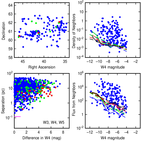
Figure 1: Results for W3, W4 and W5: (top left) Sky view of Class I sources having $22\mu$m fluxes, with color indicating luminosity range: sources within 1 magnitude of the brightest source are red, between 1 and 2 magnitudes are green, and 2 magnitudes or more fainter than the brightest are blue. (top right) Projected density in pc^-2 versus absolute source magnitude in the $22\mu$m band of WISE. Points are for $N=10$ neighbors considered in the density. Crooked lines connect the average of 3 lowest densities in each magnitude interval; dashed lines are linear fits to the crooked lines. (bottom right) Flux at the position of a protostar, measured in pc^-2, versus the absolute magnitude in the $22\mu$m band. Points are for $N=10$; crooked and dashed lines represent averages of the lowest 3 fluxes in each magnitude interval for various $N$. (bottom left) The projected separation, in pc, versus the difference in absolute magnitude, for all sources $j$ within $N=10$ neighbors of each source $i$. Colors mean the same as in the top left panel. The $12^{\prime\prime}$ FWHM at $22\mu$m is indicated by a line on the y-axis.

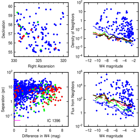
Figure 2: Results for IC 1396, as in figure 1.

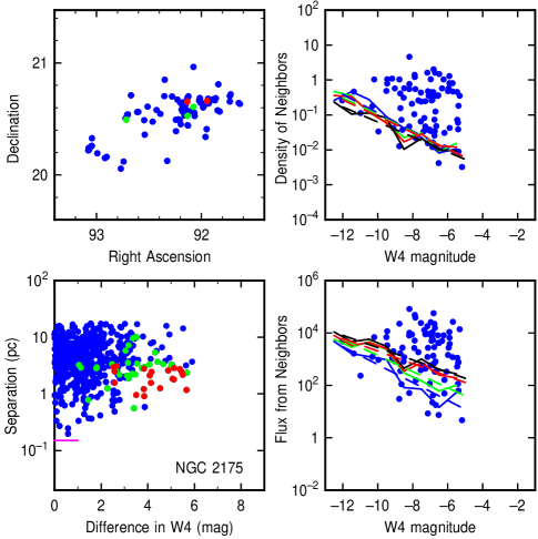
Figure 3: Results for NGC 2175, as in figure 1.

Figure 4: Slope (left) and intercept (right) of the fitted linear correlation between the minimum flux at a protostar and the protostellar absolute magnitude (bottom two panels), and the same for the minimum density (top two panels). The intercept is written as the flux or density (both in units of pc^-2) for a source with an absolute magnitude of $-10$ in the $22\mu$m band. The abscissa in each case is the number of neighboring sources used to determine the local flux or density. The purpose of this figure is to look for size-of-sample effects. The minimum flux increases with $N$ in a trivial way because larger $N$ corresponds to a larger sum of neighbor fluxes. The minimum density decreases slightly with $N$, somewhat parallel to the black line, which is the predicted size-of-sample effect for a Salpeter IMF given the average scaling between density and luminosity in figure (a) and assuming luminosity is proportional to mass.

References

- Allison et al. (2009) Allison, R. J., Goodwin, S. P., Parker, R. J., et al. 2009, MNRAS, 395, 1449
- Allison et al. (2010) Allison, R. J., Goodwin, S. P., Parker, R. J., Portegies Zwart, S. F., & de Grijs, R. 2010, MNRAS, 407, 1098
- Alves et al. (2007) Alves, J., Lombardi, M., & Lada, C. J. 2007, A&A, 462, L17
- Bate (2009) Bate, M.R. 2009, MNRAS, 392 590
- Bonnell et al. (1997) Bonnell, I. A., Bate, M. R., Clarke, C. J., & Pringle, J. E. 1997, MNRAS, 285, 201
- Bonnell & Davies (1998) Bonnell, I.A., & Davies, M.B. 1998, MNRAS, 295, 691
- Bonnell et al. (2001) Bonnell, I. A., Clarke, C. J., Bate, M. R., & Pringle, J. E. 2001, MNRAS, 324, 573
- Bonnell & Bate (2005) Bonnell, I.A., & Bate, M.R. 2005, MNRAS, 362, 915
- Bonnell & Bate (2006) Bonnell, I. A., & Bate, M. R. 2006, MNRAS, 370, 488
- Bressert et al. (2012) Bressert, E., Bastian, N., Evans, C. J., et al. 2012, A&A, 542A, 49
- de Grijs et al. (2002) de Grijs R., Gilmore G. F., Johnson R. A., & Mackey A. D., 2002, MNRAS, 331, 245
- de Wit et al. (2005) de Wit, W.J., Testi, L., Palla, F., & Zinnecker, H. 2005, A&A 437, 247
- Dunham et al. (2013) Dunham, M.M., Arce, H.G., Allen, L. et al. 2013, AJ, 145, 94
- Enoch et al. (2009) Enoch, M.L., Evans, N.J., II, Sargent, A.I., Glenn, J. 2009, ApJ, 692, 973
- Er et al. (2013) Er, X.-Y., Jiang, Z.-B., Fu, Y.-N. 2013, RAA, 13, 277
- Evans et al. (2009) Evans, N.J. II, Dunham, M.M., Jørgensen, J.K., et al. 2009, ApJS, 181, 321
- Gennaro et al. (2011) Gennaro, M., Brandner, W., Stolte, A., & Henning, Th. 2011, MNRAS, 412, 2469
- Girichidis et al. (2012) Girichidis, P., Federrath, C., Banerjee, R., & Klessen, R.S. 2012, MNRAS, 420, 613
- Goldman et al. (2013) Goldman, B., Röser, S., Schilbach, E., et al. 2013, A&A, 559, 43
- Gorti & Bhatt (1995) Gorti U. & Bhatt H. C., 1995, MNRAS, 272, 61
- Gouliermis et al. (2004) Gouliermis D., Keller S. C., Kontizas M., Kontizas E., & Bellas-Velidis I., 2004, A&A, 416, 137
- Gutermuth et al. (2009) Gutermuth, R. A., Megeath, S. T., Myers, P. C., Allen, L. E., Pipher, J. L., & Fazio, G. G. 2009, ApJS, 184, 18
- Heiderman et al. (2010) Heiderman, A., Evans, N.J., II, Allen, L.E., Huard, T., & Heyer, M. 2010, ApJ, 723, 1019
- Hillenbrand & Hartmann (1998) Hillenbrand L. A., & Hartmann L. W., 1998, ApJ, 492, 540
- Indulekha (2013) Indulekha, K. 2013, arXiv1304.1554
- Kirk & Myers (2011) Kirk H., & Myers P. C., 2011, ApJ, 727, 64
- Koenig et al. (2012) Koenig, X.P., Leisawitz, D.T., Benford, D.J., Rebull, L.M., Padgett, D.L., & Assef, R.J. ApJ, 744, 130
- Kryukova et al. (2012) Kryukova, E., Megeath, S. T., Gutermuth, R. A., Pipher, J., Allen, T. S., Allen, L. E., Myers, P. C., & Muzerolle, J. 2012, AJ, 144, 31
- Larson (1982) Larson, R.B. 1982, MNRAS, 200, 159
- Maschberger et al. (2010) Maschberger, Th., Clarke, C. J., Bonnell, I.A., Kroupa, P. 2010, MNRAS, 404, 1061
- McKee & Tan (2003) McKee, C.F., & Tan, J.C. 2003, apJ, 585, 850
- McMillan et al. (2007) McMillan, S. L. W., Vesperini, E., & Portegies Zwart, S. F. 2007, ApJL, 655, L45
- Moeckel & Bonnell (2009) Moeckel, N. & I. A. Bonnell, 2009, MNRAS, 400, 657
- Moeckel & Clarke (2011) Moeckel, N., & Clarke, C.J. 2011, MNRAS, 410, 2799
- Motte et al. (1998) Motte, F., Andre, P., & Neri, R. 1998, A&A, 336, 150
- Oey et al. (2013) Oey, M. S., Lamb, J. B., Kushner, C. T., Pellegrini, E. W., & Graus, A. S. 2013, ApJ, 768, 66, 12 pp
- Offner et al. (2009) Offner, S.S.R.. Hansen, C.E., & Krumholz, M.R. 2009, ApJL, 704, 124
- Offner & McKee (2011) Offner, S.S.R., & McKee, C.F. 2011, ApJ, 736, 53
- Olczak et al. (2011) Olczak, C., Spurzem, R., & Henning, T. 2011, A&A, 532, A119
- Pang et al. (2013) Pang, X., Grebel, E.K., Allison, R.J., Goodwin, S.P., Altmann, M., Harbeck, D., Moffat, A.F.J., & Drissen, L. 2013, ApJ, 764, 73
- Parker & Meyer (2012) Parker, R.J., & Meyer, M. R. 2012, MNRAS, 427, 637
- Pelupessy & Portegies Zwart (2012) Pelupessy, F. I., & Portegies Zwart, S. 2012, MNRAS, 420, 1503
- Portegies-Zwart & McMillan (2002) Portegies-Zwart, S. F., & McMillan, S. L. W. 2002, ApJ, 576, 899
- Prato et al. (2009) Prato, L. Lockhart, K.E., Johns-Krull, C.M., & Rayner, J.T. 2009, AJ, 137, 3931
- Rebull et al. (2010) Rebull, L. M., Padgett, D. L., McCabe, C.-E., et al. 2010, ApJS, 186, 259
- Spitzer (1940) Spitzer, L., Jr. 1940, ApJ, MNRAS, 100, 396
- Wright et al. (2010) Wright, E.L., Eisenhardt, P.R.M., Mainzer, A. et al. 2010, AJ, 140, 1868
- Yu et al. (2011) Yu, J.L., de Grijs, R., & Chen, Li. 2011, ApJ, 732, 16
- Zhang et al. (2013) Zhang, Y., Tan, J.C., De Buizer, J.M., Sandell, G., Beltran, M.T., Churchwell, E., McKee, C.F., Shuping, R., Staff, J.E., Telesco, C., Whitney, B. 2013, ApJ, 767, 58
- Zinnecker (1982) Zinnecker, H. 1982, in Glassgold, A.E. et al. eds., Symposium on the Orion Nebula to Honor Henry Draper. New York Academy of Sciences, New York, p. 226