Exact Post-Selection Inference for Sequential Regression Procedures

Abstract

We propose new inference tools for forward stepwise regression, least angle regression, and the lasso. Assuming a Gaussian model for the observation vector $y$, we first describe a general scheme to perform valid inference after any selection event that can be characterized as $y$ falling into a polyhedral set. This framework allows us to derive conditional (post-selection) hypothesis tests at any step of forward stepwise or least angle regression, or any step along the lasso regularization path, because, as it turns out, selection events for these procedures can be expressed as polyhedral constraints on $y$. The p-values associated with these tests are exactly uniform under the null distribution, in finite samples, yielding exact type I error control. The tests can also be inverted to produce confidence intervals for appropriate underlying regression parameters. The R package selectiveInference, freely available on the CRAN repository, implements the new inference tools described in this paper.
Keywords: forward stepwise regression, least angle regression, lasso, p-value, confidence interval, post-selection inference

1 Introduction

We consider observations $y\in\mathbb{R}^{n}$ drawn from a Gaussian model

$$y=\theta+\epsilon,\;\;\;\epsilon\sim N(0,\sigma^{2}I),$$ (1)

Given a fixed matrix $X\in\mathbb{R}^{n\times p}$ of predictor variables, our focus is to provide inferential tools for methods that perform variable selection and estimation in an adaptive linear regression of $y$ on $X$. Unlike much of the related literature on adaptive linear modeling, we do not assume that the true model is itself linear, i.e., we do not assume that $\theta=X\beta^{*}$ for a vector of true coefficients $\beta^{*}\in\mathbb{R}^{p}$. The particular regression models that we consider in this paper are built from sequential procedures that add (or delete) one variable at a time, such as forward stepwise regression (FS), least angle regression (LAR), and the lasso regularization path. However, we stress that the underpinnings of our approach extends well beyond these cases.

To motivate the basic problem and illustrate our proposed solutions, we examine a data set of 67 observations and 8 variables, where the outcome is the log PSA level of men who had surgery for prostate cancer. The same data set was used to motivate the covariance test in Lockhart et al. (2014). The first two numeric columns of Table 1 show the p-values for regression coefficients of variables that enter the model, across steps of FS. The first column shows the results of applying naive, ordinary t-tests to compute the significance of these regression coefficients. We see that the first four variables are apparently significant at the 0.05 level, but this is suspect, as the p-values do not account for the greedy selection of variables that is inherent to FS. The second column shows our new selection-adjusted p-values for FS, from a truncated Gaussian (TG) test developed in Sections 3 and 4. These do properly account for the greediness: they are conditional on the active set at each step, and now just two variables are significant at the 0.05 level.

	FS, naive	FS, TG		LAR, cov	LAR, spacing	LAR, TG
lcavol	0.000	0.000	lcavol	0.000	0.000	0.000
lweight	0.000	0.027	lweight	0.047	0.052	0.052
svi	0.019	0.184	svi	0.170	0.137	0.058
lbph	0.021	0.172	lbph	0.930	0.918	0.918
pgg45	0.113	0.453	pgg45	0.352	0.016	0.023
lcp	0.041	0.703	age	0.653	0.586	0.365
age	0.070	0.144	lcp	0.046	0.060	0.800
gleason	0.442	0.800	gleason	0.979	0.858	0.933

Table 1: Prostate cancer data example: p-values across steps of the forward stepwise (FS) path, computing using naive $t$-tests that do not account for greedy selection, and our new truncated Gaussian (TG) test for FS; also shown are p-values for the least angle regression (LAR) path, computed using the covariance test of Lockhart et al. (2014), and our new spacing and TG tests for LAR.

The last three numeric columns of Table 1 show analogous results for the LAR algorithm applied to the prostate cancer data (the LAR and lasso paths are identical here, as there were no variable deletions). The covariance test (Lockhart et al., 2014), reviewed in the Section 7, measures the improvement in the LAR fit due to adding a predictor at each step, and the third column shows p-values from its $\mathrm{Exp}(1)$ asymptotic null distribution. Our new framework applied to LAR, described in Section 4, produces the results in the rightmost column. We note that this TG test assumes far less than the covariance test. In fact, our TG p-values for both FS and LAR do not require assumptions about the predictors $X$, or about the true model being linear. They also use a null distribution that is correct in finite samples, rather than asymptotically, under Gaussian errors in (1). The fourth column above shows a computationally efficient approximation to the TG test for LAR, that we call the spacing test. Later, we establish an asymptotic equivalence between our new spacing for LAR and the covariance test, and this is supported by the similarity between their p-values in the table.

The R package selectiveInference provides an implementation of the TG tests for FS and LAR, and all other inference tools described in this paper. This package is available on the CRAN repository, as well as https://github.com/selective-inference/R-software. A Python implementation is also available, at https://github.com/selective-inference/Python-software.

A highly nontrivial and important question is to figure out how to combine p-values, such as those in Table 1, to build a rigorous stopping rule, i.e., a model selection rule. While we recognize its importance, this topic is not the focus of our paper. Our focus is to provide a method for computing proper p-values like those in Table 1 in the first place, which we view as a major step in the direction of answering the model selection problem in a practically and theoretically satisfactory manner. Our future work is geared more toward model selection; we also discuss this problem in more detail in Section 2.3.

1.1 Related work

There is much recent work on inference for high-dimensional regression models. One class of techniques, e.g., by Wasserman & Roeder (2009); Meinshausen & Buhlmann (2010); Minnier et al. (2011) is based on sample-splitting or resampling methods. Another class of approaches, e.g., by Zhang & Zhang (2014); Buhlmann (2013); van de Geer et al. (2014); Javanmard & Montanari (2013a, b) is based on “debiasing” or “denoising” a regularized regression estimator, like the lasso. The inferential targets considered in the aforementioned works are all fixed, and not post-selected, like the targets we study here. As we see it, it is clear (at least conceptually) how to use sample-splitting techniques to accommodate post-selection inferential goals; it is much less clear how to do so with the debiasing tools mentioned above.

Berk et al. (2013) carry out valid post-selection inference (PoSI) by considering all possible model selection procedures that could have produced the given submodel. As the authors state, the inferences are generally conservative for particular selection procedures, but have the advantage that they do not depend on the correctness of the selected submodel. This same advantage is shared by the tests we propose here. Comparisons of our tests, built for specific selection mechanisms, and the PoSI tests, which are much more general, would be interesting to pursue in future work.

Lee et al. (2013), reporting on work concurrent with that of this paper, construct p-values and intervals for lasso coefficients at a fixed value of the regularization parameter $\lambda$ (instead of a fixed number of steps $k$ along the lasso path, as we consider in Section 4). This paper and ours both leverage the same core statistical framework, using truncated Gaussian (TG) distributions, for exact post-selection inference, but differ in the applications pursued with this framework. After our work was completed, there was further progress on the application and development of exact post-selection inference tools, e.g., by Lee & Taylor (2014), Reid et al. (2014), Loftus & Taylor (2014), Choi et al. (2014), Fithian et al. (2014).

1.2 Notation and outline

Our notation in the coming sections is as follows. For a matrix $M\in\mathbb{R}^{n\times p}$ and list $S=[s_{1},\ldots s_{r}]\subseteq[1,\ldots p]$, we write $M_{S}\in\mathbb{R}^{n\times|S|}$ for the submatrix formed by extracting the corresponding columns of $M$ (in the specified order). Similarly for a vector $x\in\mathbb{R}^{p}$, we write $x_{S}$ to denote the relevant subvector. We write $(M^{T}M)^{+}$ for the (Moore-Penrose) pseudoinverse of the square matrix $M^{T}M$, and $M^{+}=(M^{T}M)^{+}M^{T}$ for the pseudoinverse of the rectangular matrix $M$. Lastly, we use $P_{L}$ for the projection operator onto a linear space $L$.

Here is an outline for the rest of this paper. Section 2 gives an overview of our main results. Section 3 describes our general framework for exact conditional inference, with truncated Gaussian (TG) test statistics. Section 4 presents applications of this framework to three sequential regression procedures: FS, LAR, and lasso. Section 5 derives a key approximation to our TG test for LAR, named the spacing test, which is considerably simpler (both in terms of form and computational requirements) than its exact counterpart. Section 6 covers empirical examples, and Section 7 draws connections between the spacing and covariance tests. We finish with a discussion in Section 8.

2 Summary of results

We now summarize our conditional testing framework, that yield the p-values demonstrated in the prostate cancer data example, beginning briefly with the general problem setting we consider. Consider testing the hypothesis

$$H_{0}:\;\,v^{T}\theta=0,$$ (2)

conditional on having observed $y\in\mathcal{P}$, where $\mathcal{P}$ is a given polyhedral set, and $v$ is a given contrast vector. We derive a test statistic $T(y,\mathcal{P},v)$ with the property that

$$T(y,\mathcal{P},v)\overset{\mathbb{P}_{0}}{\sim}\mathrm{Unif}(0,1),$$ (3)

where $\mathbb{P}_{0}(\cdot)=\mathbb{P}_{v^{T}\theta=0}(\,\cdot\,|\,y\in\mathcal{P})$, the probability measure under $\theta$ for which $v^{T}\theta=0$, conditional on $y\in\mathcal{P}$. The assertion is that $T(y,\mathcal{P},v)$ is exactly uniform under the null measure, for any finite $n$ and $p$. This statement assumes nothing about the polyhedron $\mathcal{P}$, and requires only Gaussian errors in the model (1). As it has a uniform null distribution, the test statistic in (3) serves as its own p-value, and so hereafter we will refer to it in both ways (test statistic and p-value).

Why should we concern ourselves with an event $y\in\mathcal{P}$, for a polyhedron $\mathcal{P}$? The short answer: for many regression procedures of interest—in particular, for the sequential algorithms FS, LAR, and lasso—the event that the procedure selects a given model (after a given number of steps) can be represented in this form. For example, consider FS after one step, with $p=3$ variables total: the FS procedure selects variable 3, and assigns it a positive coefficient, if and only if

$$X_{3}^{T}y/\|X_{3}\|_{2} \geq\pm X_{1}^{T}y/\|X_{1}\|_{2},$$

$$X_{3}^{T}y/\|X_{3}\|_{2} \geq\pm X_{2}^{T}y/\|X_{2}\|_{2}.$$

With $X$ considered fixed, these inequalities can be compactly represented as $\Gamma y\geq 0$, where the inequality is meant to be interpreted componentwise, and $\Gamma\in\mathbb{R}^{4\times n}$ is a matrix with rows $X_{3}/\|X_{3}\|_{2}\pm X_{1}/\|X_{1}\|_{2}$, $X_{3}/\|X_{3}\|_{2}\pm X_{2}/\|X_{2}\|_{2}$. Hence if $\hat{j}_{1}(y)$ and $\hat{s}_{1}(y)$ denote the variable and sign selected by FS at the first step, then we have shown that

$$\Big{\{}y:\hat{j}_{1}(y)=3,\,\hat{s}_{1}(y)=1\Big{\}}=\{y:\Gamma y\geq 0\},$$

for a particular matrix $\Gamma$. The right-hand side above is clearly a polyhedron (in fact, it is a cone). To test the significance of the 3rd variable, conditional on it being selected at the first step of FS, we consider the null hypothesis $H_{0}$ as in (2), with $v=X_{3}$, and $\mathcal{P}=\{y:\Gamma y\geq 0\}$. The test statistic that we construct in (3) is conditionally uniform under the null. This can be reexpressed as

$$\mathbb{P}_{X_{3}^{T}\theta=0}\Big{(}T_{1}\leq\alpha\,\Big{|}\,\hat{j}_{1}(y)=3,\,\hat{s}_{1}(y)=1\Big{)}=\alpha,$$ (4)

for all $0\leq\alpha\leq 1$. The conditioning in (4) is important because it properly accounts for the adaptive (i.e., greedy) nature of FS. Loosely speaking, it measures the magnitude of the linear function $v_{3}^{T}y$—not among all $y$ marginally—but among the vectors $y$ that would result in FS selecting variable 3, and assigning it a positive coefficient.

A similar construction holds for a general step $k$ of FS: letting $\hat{A}_{k}(y)=[\hat{j}_{1}(y),\ldots\hat{j}_{k}(y)]$ denote the active list after $k$ steps (so that FS selects these variables in this order) and $\hat{s}_{A_{k}}(y)=[\hat{s}_{1}(y),\ldots\hat{s}_{k}(y)]$ denote the signs of the corresponding coefficients, we have, for any fixed $A_{k}$ and $s_{A_{k}}$,

$$\Big{\{}y:\hat{A}_{k}(y)=A_{k},\,\hat{s}_{A_{k}}(y)=s_{A_{k}}\Big{\}}=\{y:\Gamma y\geq 0\},$$

for another matrix $\Gamma$. With $v=(X_{A_{k}}^{+})^{T}e_{k}$, where $e_{k}$ is the $k$th standard basis vector, the hypothesis in (2) is $e_{k}^{T}X_{A_{k}}^{+}\theta=0$, i.e., it specifies that the last partial regression coefficient is not significant, in a projected linear model of $\theta$ on $X_{A_{k}}$. For $\mathcal{P}=\{y:\Gamma y\geq 0\}$, the test statistic in (3) has the property

$$\mathbb{P}_{e_{k}^{T}X_{A_{k}}^{+}\theta=0}\Big{(}T_{k}\leq\alpha\,\Big{|}\,\hat{A}_{k}(y)=A_{k},\,\hat{s}_{A_{k}}(y)=s_{A_{k}}\Big{)}=\alpha,$$ (5)

for all $0\leq\alpha\leq 1$. We emphasize that the p-value in (5) is exactly (conditionally) uniform under the null, in finite samples. This is true without placing any restrictions on $X$ (besides a general position assumption), and notably, without assuming linearity of the underlying model (i.e., without assuming $\theta=X\beta^{*}$). Further, though we described the case for FS here, essentially the same story holds for LAR and lasso. The TG p-values for FS and LAR in Table 1 correspond to tests of hypotheses as in (5), i.e., tests of $e_{k}^{T}X_{A_{k}}^{+}\theta=0$, over steps of these procedures.

An important point to keep in mind throughout is that our testing framework for the sequential FS, LAR, and lasso procedures is not specific to the choice $v=(X_{A_{k}}^{+})^{T}e_{k}$, and allows for the testing of arbitrary linear contrasts $v^{T}\theta$ (as long as $v$ is fixed by the conditioning event). For concreteness, we will pay close attention to the case $v=(X_{A_{k}}^{+})^{T}e_{k}$, since it gives us a test for the significance of variables as they enter the model, but many other choices of $v$ could be interesting and useful.

2.1 Conditional confidence intervals

A strength of our framework is that our test statistics can be inverted to make coverage statements about arbitrary linear contrasts of $\theta$. In particular, consider the hypothesis test defined by $v=(X_{A_{k}}^{+})^{T}e_{k}$, for the $k$th step of FS (similar results apply to LAR and lasso). By inverting our test statistic in (5), we obtain a conditional confidence interval $I_{k}$ satisfying

$$\mathbb{P}\Big{(}e_{k}^{T}X_{A_{k}}^{+}\theta\in I_{k}\,\Big{|}\,\hat{A}_{k}(y)=A_{k},\,\hat{s}_{A_{k}}(y)=s_{A_{k}}\Big{)}=1-\alpha.$$ (6)

In words, the random interval $I_{k}$ traps with probability $1-\alpha$ the coefficient of the last selected variable, in a regression model that projects $\theta$ onto $X_{A_{k}}$, conditional on FS having selected variables $A_{k}$ with signs $s_{A_{k}}$, after $k$ steps of the algorithm. As (6) is true conditional on $\Gamma y\geq 0$, we can also marginalize this statement to yield

$$\mathbb{P}\Big{(}e_{k}^{T}X_{\hat{A}_{k}}^{+}\theta\in I_{k}\Big{)}=1-\alpha.$$ (7)

Note that $\hat{A}_{k}=\hat{A}_{k}(y)$ denotes the random active list after $k$ FS steps. Written in the unconditional form (7), we call $I_{k}$ a selection interval for the random quantity $e_{k}^{T}X_{\hat{A}_{k}}^{+}\theta$. We use this name to emphasize the difference in interpretation here, versus the conditional case: the selection interval covers a moving target, as both the identity of the $k$th selected variable, and the identities of all the previously selected variables (which play a role in the $k$th partial regression coefficient of $\theta$ on $X_{\hat{A}_{k}}$), are random—they depend on $y$.

We have seen that our intervals can be interpreted conditionally, as in (6), or unconditionally, as in (7). The former is perhaps more aligned with the spirit of post-selection inference, as it guarantees coverage, conditional on the output of our selection procedure. But the latter interpretation is also interesting, and in a way, cleaner. From the unconditional point of view, we can roughly think of the selection interval $I_{k}$ as covering the project population coefficient of the “$k$th most important variable” as deemed by the sequential regression procedure at hand (FS, LAR, or lasso). Figure 1 displays 90% confidence intervals at each step of FS, run on the prostate cancer data set discussed in the introduction.

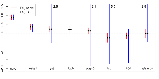
Figure 1: Prostate cancer data example: naive confidence intervals and 90% conditional confidence intervals (or, selection intervals) computed using the TG (truncated Gaussian) statistics, for FS (forward stepwise). Black dots denote the estimated partial regression coefficients for the variable to enter, in a regression on the active submodel. The upper confidence limits for some parameters exceed the range for the y-axis on the plot, and their actual values marked at the appropriate places.

2.2 Marginalization

Similar to the formation of selection intervals in the last subsection, we note that any amount of coarsening, i.e., marginalization, of the conditioning set in (5) results in a valid interpretation for p-values. For example, by marginalizing over all possible sign lists $s_{A_{k}}$ associated with $A_{k}$, we obtain

$$\mathbb{P}_{e_{k}^{T}X_{A_{k}}^{+}\theta=0}\Big{(}T_{k}\leq\alpha\,\Big{|}\,\hat{A}_{k}(y)=A_{k}\Big{)}=\alpha,$$

so that the conditioning event only encodes the observed active list, and not the observed signs. Thus we have another possible interpretation for the statistic (p-value) $T_{k}$: under the null measure, which conditions on FS having selected the variables $A_{k}$ (regardless of their signs), $T_{k}$ is uniformly distributed. The idea of marginalization will be important when we discuss details of the constructed tests for LAR and lasso.

2.3 Model selection

How can the inference tools of this paper be translated into rigorous rules for model selection? This is of course an important (and difficult) question, and we do not yet possess a complete understanding of the model selection problem, though it is the topic of future work. Below we describe three possible strategies for model selection, using the p-values that come from our inference framework. We do not have extensive theory to explain or evaluate them, but all are implemented in the R package selectiveInference.

• Inference from sequential p-values. We have advocated the idea of computing p-values across steps of the regression procedure at hand, as exemplified in Table 1. Here at each step $k$, the p-value tests $e_{k}^{T}X_{A_{k}}^{+}\theta=0$, i.e., tests the significance of the variable to enter the active set $A_{k}$, in a projected linear model of the mean $\theta$ on the variables in $A_{k}$. G’Sell et al. (2015) propose sequential stopping rules using such p-values, including the “ForwardStop” rule, which guarantees false discovery rate (FDR) control at a given level. For example, the ForwardStop rule at a nominal 10% FDR level, applied to the TG p-values from the LAR path for the prostate cancer data (the last column of Table 1), yields a model with 3 predictors. However, it should be noted that the guarantee for FDR control for ForwardStop in G’Sell et al. (2015) assumes that the p-values are independent, and this is not true for the p-values from our inference framework.

• Inference at a fixed step $k$. Instead of looking at p-values across steps, we could instead fix a step $k$, and inspect the p-values corresponding to the hypotheses $e_{j}^{T}X_{A_{j}}^{+}\theta=0$, for $j=1,\ldots k$. This tests the significance of every variable, among the rest in the discovered active set $A_{k}$, and it still fits within our developed framework: we are just utilizing different linear contrasts $v=(X_{A_{j}}^{+})^{T}e_{j}$ of the mean $\theta$, for $j=1,\ldots k$. The results of these tests are genuinely different, in terms of their statistical meaning, than the results from testing variables as they enter the model (since the active set changes at each step). Given the p-values corresponding to all active variables at a given step $k$, we could, e.g., perform a Bonferroni correction, and declare significance at the level $\alpha/k$, in order to select a model (a subset of $A_{k}$) with type I error controlled at the level $\alpha$. For example, when we apply this strategy at step $k=5$ of the LAR path for the prostate cancer data, and examine Bonferroni corrected p-values at the 0.05 level, only two predictors (lweight and pgg45) end up being significant.

• Inference at an adaptively selected step $k$. Lastly, the above scheme for inference could be conducted with a step number $k$ that is adaptively selected, instead of fixed ahead of time, provided the selection event that determines $k$ is a polyhedral set in $y$. A specific example of this is an AIC-style rule, which chooses the step $k$ after which the AIC criterion rises, say, twice in a row. We omit the details, but verifying that such a stopping rule defines a polyhedral constraint for $y$ is straightforward (it follows essentially the same logic as the arguments that show the FS selection event is itself polyhedral, which are given in Section 4.1). Hence, by including all the necessary polyhedral constraints—those that determine $k$, and those that subsequently determine the selected model—we can compute p-values for each of the active variables at an adaptively selected step $k$, using the inference tools derived in this paper. When this method is applied to the prostate cancer data set, the AIC-style rule (which stops once it sees two consecutive rises in the AIC criterion) chooses $k=4$. Examining Bonferroni corrected p-values at step $k=4$, only one predictor (lweight) remains significant at the 0.05 level.

3 Conditional Gaussian inference after polyhedral selection

In this section, we present a few key results on Gaussian contrasts conditional on polyhedral events, which provides a basis for the methods proposed in this paper. The same core development appears in Lee et al. (2013); for brevity, we refer the reader to the latter paper for formal proofs. We assume $y\sim N(\theta,\Sigma)$, where $\theta\in\mathbb{R}^{n}$ is unknown, but $\Sigma\in\mathbb{R}^{n\times n}$ is known. This generalizes our setup in (1) (allowing for a general error covariance matrix). We also consider a generic polyhedron $\mathcal{P}=\{y:\Gamma y\geq u\}$, where $\Gamma\in\mathbb{R}^{m\times n}$ and $u\in\mathbb{R}^{m}$ are fixed, and the inequality is to be interpreted componentwise. For a fixed $v\in\mathbb{R}^{n}$, our goal is to make inferences about $v^{T}\theta$ conditional on $y\in\mathcal{P}$. Next, we provide a helpful alternate representation for $\mathcal{P}$.

Lemma 1 (Polyhedral selection as truncation).

For any $\Sigma,v$ such that $v^{T}\Sigma v\not=0$,

$$\Gamma y\geq u\iff\mathcal{V}^{\mathrm{lo}}(y)\leq v^{T}y\leq\mathcal{V}^{\mathrm{up}}(y),\,\mathcal{V}^{0}(y)\leq 0,$$ (8)

where

$$\mathcal{V}^{\mathrm{lo}}(y) =\max_{j:\rho_{j}>0}\,\frac{u_{j}-(\Gamma y)_{j}+\rho_{j}v^{T}y}{\rho_{j}},$$ (9)

$$\mathcal{V}^{\mathrm{up}}(y) =\min_{j:\rho_{j}<0}\,\frac{u_{j}-(\Gamma y)_{j}+\rho_{j}v^{T}y}{\rho_{j}},$$ (10)

$$\mathcal{V}^{0}(y) =\max_{j:\rho_{j}=0}\,u_{j}-(\Gamma y)_{j},$$ (11)

and $\rho=\Gamma\Sigma v/v^{T}\Sigma v$. Moreover, the triplet $(\mathcal{V}^{\mathrm{lo}},\mathcal{V}^{\mathrm{up}},\mathcal{V}^{0})(y)$ is independent of $v^{T}y$.

Remark 1.

The result in (8), with $\mathcal{V}^{\mathrm{lo}},\mathcal{V}^{\mathrm{up}},\mathcal{V}^{0}$ defined as in (9)–(11), is a deterministic result that holds for all $y$. Only the last independence result depends on normality of $y$.

See Figure 2 for a geometric illustration of this lemma. Intuitively, we can explain the result as follows, assuming for simplicity (and without a loss of generality) that $\Sigma=I$. We first decompose $y=P_{v}y+P_{v^{\perp}}y$, where $P_{v}y=vv^{T}y/\|v\|^{2}_{2}$ is the projection of $y$ along $v$, and $P_{v^{\perp}}y=y-P_{v}y$ is the projection onto the orthocomplement of $v$. Accordingly, we view $y$ as a deviation from $P_{v^{\perp}}y$, of an amount $v^{T}y$, along the line determined by $v$. The quantities $\mathcal{V}^{\mathrm{lo}}$ and $\mathcal{V}^{\mathrm{up}}$ describe how far we can deviate on either side of $P_{v^{\perp}}y$, before $y$ leaves the polyhedron. This gives rise to the inequality $\mathcal{V}^{\mathrm{lo}}\leq v^{T}y\leq\mathcal{V}^{\mathrm{up}}$. Some faces of the polyhedron, however, may be perfectly aligned with $v$ (i.e., their normal vectors may be orthogonal to $v$), and $\mathcal{V}^{0}$ accounts for this by checking that $y$ lies on the correct side of these faces.

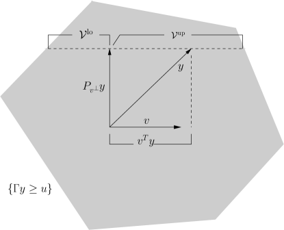
Figure 2: Geometry of polyhedral selection as truncation. For simplicity, we assume that $\Sigma=I$ (otherwise standardize as appropriate). The shaded gray area is the polyhedral set $\{y:\Gamma y\geq u\}$. By breaking up $y$ into its projection onto $v$ and its projection onto the orthogonal complement of $v$, we see that $\Gamma y\geq u$ holds if and only if $v^{T}y$ does not deviate too far from $P_{v^{\perp}}y$, hence trapping it in between bounds $\mathcal{V}^{\mathrm{lo}},\mathcal{V}^{\mathrm{up}}$. Furthermore, these bounds $\mathcal{V}^{\mathrm{lo}},\mathcal{V}^{\mathrm{up}}$ are functions of $P_{v^{\perp}}y$ alone, so under normality, they are independent of $v^{T}y$.

From Lemma 1, the distribution of any linear function $v^{T}y$, conditional on the selection $\Gamma y\geq u$, can be written as the conditional distribution

$$v^{T}y\,\big{|}\,\mathcal{V}^{\mathrm{lo}}(y)\leq v^{T}y\leq\mathcal{V}^{\mathrm{up}}(y),\,\mathcal{V}^{0}(y)\leq 0.$$ (12)

Since $v^{T}y$ has a Gaussian distribution, the above is a truncated Gaussian distribution (with random truncation limits). A simple transformation leads to a pivotal statistic, which will be critical for inference about $v^{T}\theta$.

Lemma 2 (Pivotal statistic after polyhedral selection).

Let $\Phi(x)$ denote the standard normal cumulative distribution function (CDF), and let $F_{\mu,\sigma^{2}}^{[a,b]}$ denote the CDF of a $N(\mu,\sigma^{2})$ random variable truncated to lie in $[a,b]$, i.e.,

$$F_{\mu,\sigma^{2}}^{[a,b]}(x)=\frac{\Phi((x-\mu)/\sigma)-\Phi((a-\mu)/\sigma)}{\Phi((b-\mu)/\sigma)-\Phi((a-\mu)/\sigma)}.$$

For $v^{T}\Sigma v\not=0$, the statistic $F_{v^{T}\theta,v^{T}\Sigma v}^{[\mathcal{V}^{\mathrm{lo}},\mathcal{V}^{\mathrm{up}}]}(v^{T}y)$ is a pivotal quantity conditional on $\Gamma y\geq u$:

$$\mathbb{P}\Big{(}F_{v^{T}\theta,v^{T}\Sigma v}^{[\mathcal{V}^{\mathrm{lo}},\mathcal{V}^{\mathrm{up}}]}(v^{T}y)\leq\alpha\,\Big{|}\,\Gamma y\geq u\Big{)}=\alpha,$$ (13)

for any $0\leq\alpha\leq 1$, where $\mathcal{V}^{\mathrm{lo}}$, $\mathcal{V}^{\mathrm{up}}$ are as defined in (9), (10).

Remark 2.

A referee of this paper astutely noted the connection between Lemma 2 and classic results on inference in an exponential family model (e.g., Chapter 4 of Lehmann & Romano (2005)), in the presence of nuisance parameters. The analogy is, in a rotated coordinate system, the parameter of interest is $v^{T}\theta$, and the nuisance parameters correspond to $P_{v}^{\perp}\theta$. This connection is developed in Fithian et al. (2014).

The pivotal statistic in the lemma leads to valid conditional p-values for testing the null hypothesis $H_{0}:v^{T}\theta=0$, and correspondingly, conditional confidence intervals for $v^{T}\theta$. We divide our presentation into two parts, on one-sided and two-sided inference.

3.1 One-sided conditional inference

The result below is a direct consequence of the pivot in Lemma 2.

Lemma 3 (One-sided conditional inference after polyhedral selection).

Given $v^{T}\Sigma v\not=0$, suppose that we are interested in testing

$$H_{0}:\;\,v^{T}\theta=0\;\;\;\text{against}\;\;\;H_{1}:\;\,v^{T}\theta>0.$$

Define the test statistic

$$T=1-F_{0,v^{T}\Sigma v}^{[\mathcal{V}^{\mathrm{lo}},\mathcal{V}^{\mathrm{up}}]}(v^{T}y),$$ (14)

where we use the notation of Lemma 2 for the truncated normal CDF. Then $T$ is a valid p-value for $H_{0}$, conditional on $\Gamma y\geq u$:

$$\mathbb{P}_{v^{T}\theta=0}(T\leq\alpha\,|\,\Gamma y\geq u)=\alpha,$$ (15)

for any $0\leq\alpha\leq 1$. Further, define $\delta_{\alpha}$ to satisfy

$$1-F_{\delta_{\alpha},v^{T}\Sigma v}^{[\mathcal{V}^{\mathrm{lo}},\mathcal{V}^{\mathrm{up}}]}(v^{T}y)=\alpha.$$ (16)

Then $I=[\delta_{\alpha},\infty)$ is a valid one-sided confidence interval for $v^{T}\theta$, conditional on $\Gamma y\geq u$:

$$\mathbb{P}(v^{T}\theta\geq\delta_{\alpha}\,|\,\Gamma y\geq u)=1-\alpha.$$ (17)

Note that by defining our test statistic in terms of the conditional survival function, as in (14), we are implicitly aligning ourselves to have power against the one-sided alternative $H_{1}:v^{T}\theta>0$. This is because the truncated normal survival function $1-F_{\mu,\sigma^{2}}^{[a,b]}(x)$, evaluated at any fixed point $x$, is monotone increasing in $\mu$. The same fact (monotonicity of the survival function in $\mu$) validates the coverage of the constructed confidence interval in (16), (17).

3.2 Two-sided conditional inference

For a two-sided alternative, we use a simple modification of the one-sided test in Lemma 3.

Lemma 4 (Two-sided conditional inference after polyhedral selection).

Given $v^{T}\Sigma v\not=0$, suppose that we are interested in testing

$$H_{0}:\;\,v^{T}\theta=0\;\;\;\text{against}\;\;\;H_{1}:\;\,v^{T}\theta\not=0.$$

Define the test statistic

$$T=2\cdot\min\Big{\{}F_{0,v^{T}\Sigma v}^{[\mathcal{V}^{\mathrm{lo}},\mathcal{V}^{\mathrm{up}}]}(v^{T}y),\;1-F_{0,v^{T}\Sigma v}^{[\mathcal{V}^{\mathrm{lo}},\mathcal{V}^{\mathrm{up}}]}(v^{T}y)\Big{\}},$$ (18)

where we use the notation of Lemma 2 for the truncated normal CDF. Then $T$ is a valid p-value for $H_{0}$, conditional on $\Gamma y\geq u$:

$$\mathbb{P}_{v^{T}\theta=0}(T\leq\alpha\,|\,\Gamma y\geq u)=\alpha,$$ (19)

for any $0\leq\alpha\leq 1$. Further, define $\delta_{\alpha/2},\delta_{1-\alpha/2}$ to satisfy

$$1-F_{\delta_{\alpha/2},v^{T}\Sigma v}^{[\mathcal{V}^{\mathrm{lo}},\mathcal{V}^{\mathrm{up}}]}(v^{T}y) =\alpha/2,$$ (20)

$$1-F_{\delta_{1-\alpha/2},v^{T}\Sigma v}^{[\mathcal{V}^{\mathrm{lo}},\mathcal{V}^{\mathrm{up}}]}(v^{T}y) =1-\alpha/2.$$ (21)

Then

$$\mathbb{P}(\delta_{\alpha/2}\leq v^{T}\theta\leq\delta_{1-\alpha/2}\,|\,\Gamma y\geq u)=1-\alpha.$$ (22)

The test statistic in (18), defined in terms of the minimum of the truncated normal CDF and survival function, has power against the two-sided alternative $H_{1}:v^{T}\theta\not=0$. The proof of its null distribution in (19) follows from the simple fact that if $U$ is a standard uniform random variable, then so is $2\cdot\min\{U,1-U\}$. The construction of the confidence interval in (20), (21), (22) again uses the monotonicity of the truncated normal survival function in the underlying mean parameter.

4 Exact selection-adjusted tests for FS, LAR, lasso

Here we apply the tools of Section 3 to the case of selection in regression using the forward stepwise (FS), least angle regression (LAR), or lasso procedures. We assume that the columns of $X$ are in general position. This means that for any $k<\min\{n,p\}$, any subset of columns $X_{j_{1}},\ldots X_{j_{k}}$, and any signs $\sigma_{1},\ldots\sigma_{k}\in\{-1,1\}$, the affine span of $\sigma_{1}X_{j_{1}},\ldots\sigma_{k}X_{j_{k}}$ does not contain any of the remaining columns, up to a sign flip (i.e., does not contain any of $\pm X_{j}$, $j\not=j_{1},\ldots j_{k}$). One can check that this implies the sequence of FS estimates is unique. It also implies that the LAR and lasso paths of estimates are uniquely determined (Tibshirani, 2013). The general position assumption is not at all stringent; e.g., if the columns of $X$ are drawn according to a continuous probability distribution, then they are in general position almost surely.

Next, we show that the model selection events for FS, LAR, and lasso can be characterized as polyhedra (indeed, cones) of the form $\{y:\Gamma y\geq 0\}$. After this, we describe the forms of the exact conditional tests and intervals, as provided by Lemmas 1–4, for these procedures, and discuss some important practical issues.

4.1 Polyhedral sets for FS selection events

Recall that FS repeatedly adds the predictor to the current active model that most improves the fit. After each addition, the active coefficients are recomputed by least squares regression on the active predictors. This process ends when all predictors are in the model, or when the residual error is zero.

Formally, suppose that $A_{k}=[j_{1},\ldots j_{k}]$ is the list of active variables selected by FS after $k$ steps, and $s_{A_{k}}=[s_{1},\ldots s_{k}]$ denotes their signs upon entering. That is, at each step $k$, the variable $j_{k}$ and sign $s_{k}$ satisfy

$$\mathrm{RSS}\big{(}y,X_{[j_{1},\ldots j_{k-1},j_{k}]}\big{)} \leq\mathrm{RSS}\big{(}y,X_{[j_{1},\ldots j_{k-1},j]}\big{)}\;\;\;\text{for all $j\not=j_{1},\ldots j_{k}$, and}$$

$$s_{k} ={\mathrm{sign}}\big{(}e_{k}^{T}(X_{[j_{1},\ldots j_{k}]})^{+}y\big{)},$$

where $\mathrm{RSS}(y,X_{S})$ denotes the residual sum of squares from regressing $y$ onto $X_{S}$, for a list of variables $S$.

The set of all observations vectors $y$ that give active list $A_{k}$ and sign list $s_{A_{k}}$ over $k$ steps, denoted

$$\mathcal{P}=\Big{\{}y:\hat{A}_{k}(y)=A_{k},\,\hat{s}_{A_{k}}(y)=s_{A_{k}}\Big{\}},$$ (23)

is indeed a polyhedron of the form $\mathcal{P}=\{y:\Gamma y\geq 0\}$. The proof of this fact uses induction. The case when $k=1$ can be seen directly by inspection, as $j_{1}$ and $s_{1}$ are the variable and sign to be chosen by FS if and only if

$$\Big{\|}\Big{(}I-X_{j_{1}}X_{j_{1}}^{T}/\|X_{j_{1}}\|_{2}^{2}\Big{)}y\Big{\|}_{2}^{2} \leq\Big{\|}\Big{(}I-X_{j}X_{j}^{T}/\|X_{j}\|_{2}^{2}\Big{)}y\Big{\|}_{2}^{2}\;\;\;\text{for all $j\not=j_{1}$, and}$$

$$s_{1} ={\mathrm{sign}}(X_{j_{1}}^{T}y),$$

which is equivalent to

$$s_{1}X_{j_{1}}^{T}y/\|X_{j_{1}}\|_{2}\geq\pm X_{j}^{T}y/\|X_{j}\|_{2}\;\;\;\text{for all $j\not=j_{1}$}.$$

Thus the matrix $\Gamma$ begins with $2(p-1)$ rows of the form $s_{1}X_{j_{1}}/\|X_{j_{1}}\|_{2}\pm X_{j}/\|X_{j}\|_{2}$, for $j\not=j_{1}$. Now assume the statement is true for $k-1$ steps. At step $k$, the optimality conditions for $j_{k},s_{k}$ can be expressed as

$$\Big{\|}\Big{(}I-\tilde{X}_{j_{k}}\tilde{X}_{j_{k}}^{T}/\|\tilde{X}_{j_{k}}\|_{2}^{2}\Big{)}r\Big{\|}_{2}^{2} \leq\Big{\|}\Big{(}I-\tilde{X}_{j}\tilde{X}_{j}^{T}/\|\tilde{X}_{j}\|_{2}^{2}\Big{)}r\Big{\|}_{2}^{2}\;\;\;\text{for all $j\not=j_{1},\ldots j_{k}$, and}$$

$$s_{k} ={\mathrm{sign}}(\tilde{X}_{j_{k}}^{T}r),$$

where $\tilde{X}_{j}$ denotes the residual from regressing $X_{j}$ onto $X_{A_{k-1}}$, and $r$ the residual from regressing $y$ onto $X_{A_{k-1}}$. As in the $k=1$ case, the above is equivalent to

$$s_{k}\tilde{X}_{j_{k}}^{T}r/\|\tilde{X}_{j_{k}}\|_{2}\geq\pm\tilde{X}_{j}^{T}r/\|\tilde{X}_{j}\|_{2}\;\;\;\text{for all $j\not=j_{1},\ldots j_{k}$},$$

or

$$s_{k}X_{j_{k}}^{T}P^{\perp}_{A_{k-1}}y/\|P^{\perp}_{A_{k-1}}X_{j_{k}}\|_{2}\geq\pm X_{j}^{T}P^{\perp}_{A_{k-1}}y/\|P^{\perp}_{A_{k-1}}X_{j}\|_{2}\;\;\;\text{for all $j\not=j_{1},\ldots j_{k}$},$$

where $P^{\perp}_{A_{k-1}}$ denotes the projection orthogonal to the column space of $X_{A_{k-1}}$. Hence we append $2(p-k)$ rows to $\Gamma$, of the form $P^{\perp}_{A_{k-1}}(s_{k}X_{j_{k}}/\|P^{\perp}_{A_{k-1}}X_{j_{k}}\|_{2}\pm X_{j}/\|P^{\perp}_{A_{k-1}}X_{j}\|_{2})$, for $j\not=j_{1},\ldots j_{k}$. In summary, after $k$ steps, the polyhedral set for the FS selection event (23) corresponds to a matrix $\Gamma$ with $2pk-k^{2}-k$ rows.

4.2 Polyhedral sets for LAR selection events

The LAR algorithm (Efron et al., 2004) is an iterative method, like FS, that produces a sequence of nested regression models. As before, we keep a list of active variables and signs across steps of the algorithm. Here is a concise description of the LAR steps. At step $k=1$, we initialize the active variable and sign list with $A=[j_{1}]$ and $s_{A_{1}}=[s_{1}]$, where $j_{1},s_{1}$ satisfy

$$(j_{1},s_{1})=\mathop{\mathrm{argmax}}_{j=1,\ldots p,\,s\in\{-1,1\}}\,sX_{j}^{T}y.$$ (24)

(This is the same selection as made by FS at the first step, provided that $X$ has columns with unit norm.) We also record the first knot

$$\lambda_{1}=s_{1}X_{j_{1}}^{T}y.$$ (25)

For a general step $k>1$, we form the list $A_{k}$ by appending $j_{k}$ to $A_{k-1}$, and form $s_{A_{k}}$ by appending $s_{k}$ to $s_{A_{k-1}}$, where $j_{k},s_{k}$ satisfy

$$(j_{k},s_{k})=\mathop{\mathrm{argmax}}_{j\notin{A_{k-1}},\,s\in\{-1,1\}}\,\frac{X_{j}^{T}P^{\perp}_{A_{k-1}}y}{s-X_{j}^{T}(X_{A_{k-1}}^{+})^{T}s_{A_{k-1}}}\cdot 1\left\{\frac{X_{j}^{T}P^{\perp}_{A_{k-1}}y}{s-X_{j}^{T}(X_{A_{k-1}}^{+})^{T}s_{A_{k-1}}}\leq\lambda_{k-1}\right\}.$$ (26)

Above, $P^{\perp}_{A_{k-1}}$ is the projection orthogonal to the column space of $X_{A_{k-1}}$, $1\{\cdot\}$ denotes the indicator function, and $\lambda_{k-1}$ is the knot value from step $k-1$. We also record the $k$th knot

$$\lambda_{k}=\frac{X_{j_{k}}^{T}P^{\perp}_{A_{k-1}}y}{s_{k}-X_{j_{k}}^{T}(X_{A_{k-1}}^{+})^{T}s_{A_{k-1}}}.$$ (27)

The algorithm terminates after the $k$-step model if $k=p$, or if $\lambda_{k+1}<0$.

LAR is often viewed as “less greedy” than FS. It is also intimately tied to the lasso, as covered in the next subsection. Now, we verify that the LAR selection event

$$\mathcal{P}=\Big{\{}y:\hat{A}_{k}(y)=A_{k},\,\hat{s}_{A_{k}}(y)=s_{A_{k}},\,\hat{S}_{\ell}(y)=S_{\ell},\,\ell=1,\ldots k\Big{\}}$$ (28)

is a polyhedron of the form $\mathcal{P}=\{y:\Gamma y\geq 0\}$. We can see that the LAR event in (28) contains “extra” conditioning, $\hat{S}_{\ell}(y)=S_{\ell}$, $\ell=1,\ldots k$, when compared to the FS event in (23). Explained in words, $S_{\ell}\subseteq\{1,\ldots p\}\times\{-1,1\}$ contains the variable-sign pairs that were “in competition” to become the active variable-sign pair step $\ell$. A subtlety of LAR: it is not always the case that $S_{\ell}=A_{\ell-1}^{c}\times\{-1,1\}$, since some variable-sign pairs are automatically excluded from consideration, as they would have produced a knot value that is too large (larger than the previous knot $\lambda_{\ell-1}$). This is reflected by the indicator function in (26). The characterization in (28) is still perfectly viable for inference, because any conditional statement over $\mathcal{P}$ in (28) translates into a valid one without conditioning on $\hat{S}_{\ell}(y)$, $\ell=1,\ldots k$, by marginalizing over all possible realizations $S_{\ell}$, $\ell=1,\ldots k$. (Recall the discussion of marginalization in Section 2.2.)

The polyhedral representation for $\mathcal{P}$ in (28) again proceeds by induction. Starting with $k=1$, we can express the optimality of $j_{1},s_{1}$ in (24) as

$$c(j_{1},s_{1})^{T}y\geq c(j,s)^{T}y,\;\;\;\text{for all $j\not=j_{1}$, $s\in\{-1,1\}$},$$

where $c(j,s)=sX_{j}$. Thus $\Gamma$ has $2(p-1)$ rows, of the form $c(j_{1},s_{1})-c(j,s)$ for $j\not=j_{1}$, $s\in\{-1,1\}$. (In the first step, $S_{1}=\{1,\ldots p\}\times\{-1,1\}$, and we do not require extra rows of $\Gamma$ to explicitly represent it.) Further, suppose that the selection set can be represented in the desired manner, after $k-1$ steps. Then the optimality of $j_{k},s_{k}$ in (26) can be expressed as

$$c(j_{k},s_{k},A_{k-1},s_{A_{k-1}})^{T}y \geq c(j,s,A_{k-1},s_{A_{k-1}})^{T}y\;\;\;\text{for all $(j,s)\in S_{k}\setminus\{(j_{k},s_{k})\}$},$$

$$c(j_{k},s_{k},A_{k-1},s_{A_{k-1}})^{T}y \geq 0,$$

where $c(j,s,A_{k-1},s_{A_{k-1}})=(P^{\perp}_{A_{k-1}}X_{j})/(s-X_{j}^{T}(X_{A_{k-1}}^{+})^{T}s_{A_{k-1}})$. The set $S_{k}$ is characterized by

$$c(j,s,A_{k-1},s_{A_{k-1}})^{T}y \leq\lambda_{k-1}\;\;\;\text{for $(j,s)\in S_{k}$},$$

$$c(j,s,A_{k-1},s_{A_{k-1}})^{T}y \geq\lambda_{k-1}\;\;\;\text{for $(j,s)\in\big{(}A_{k-1}^{c}\times\{-1,1\}\big{)}\setminus S_{k}$}.$$

Notice that $\lambda_{k-1}=c(j_{k-1},s_{k-1},A_{k-2},s_{A_{k-2}})^{T}y$ is itself a linear function of $y$, by the inductive hypothesis. Therefore, the new $\Gamma$ matrix is created by appending the following $|S_{k}|+2(p-k+1)$ rows to the previous matrix: $c(j_{k},s_{k},A_{k-1},s_{A_{k-1}})-c(j,s,A_{k-1},s_{A_{k-1}})$, for $(j,s)\in S_{k}\setminus\{(j_{k},s_{k})\}$; $c(j_{k},s_{k},A_{k-1},s_{A_{k-1}})$; $c(j_{k-1},s_{k-1},A_{k-2},s_{A_{k-2}})-c(j,s,A_{k-1},s_{A_{k-1}})$, for $(j,s)\in S_{k}$; $c(j,s,A_{k-1},s_{A_{k-1}})-c(j_{k-1},s_{k-1},A_{k-2},s_{A_{k-2}})$ for $(j,s)\in(A_{k-1}^{c}\times\{-1,1\})\setminus S_{k}$. In total, the number of rows of $\Gamma$ at step $k$ of LAR is bounded above by $\sum_{\ell=1}^{k}(|S_{\ell}|+2(p-\ell+1))\leq 3pk-3k^{2}/2+3k/2$.

4.3 Polyhedral sets for lasso selection events

By introducing a step into the LAR algorithm that deletes variables from the active set if their coefficients pass through zero, the modified LAR algorithm traces out the lasso regularization path (Efron et al., 2004). To concisely describe this modification, at a step $k>1$, denote by $(j_{k}^{\mathrm{add}},s_{k}^{\mathrm{add}})$ the variable-sign pair to enter the model next, as defined in (26), and denote by $\lambda_{k}^{\mathrm{add}}$ the value of $\lambda$ at which they would enter, as defined in (27). Now define

$$j_{k}^{\mathrm{del}}=\mathop{\mathrm{argmax}}_{j\in A_{k-1}\setminus\{j_{k-1}\}}\,\frac{e_{j}^{T}X_{A_{k-1}}^{+}y}{e_{j}^{T}(X_{A_{k-1}}^{T}X_{A_{k-1}})^{-1}s_{A_{k-1}}}\cdot 1\left\{\frac{e_{j}^{T}X_{A_{k-1}}^{+}y}{e_{j}^{T}(X_{A_{k-1}}^{T}X_{A_{k-1}})^{-1}s_{A_{k-1}}}\leq\lambda_{k-1}\right\},$$ (29)

the variable to leave the model next, and

$$\lambda_{k}^{\mathrm{del}}=\frac{e_{j_{k}^{\mathrm{del}}}^{T}X_{A_{k-1}}^{+}y}{e_{j_{k}^{\mathrm{del}}}^{T}(X_{A_{k-1}}^{T}X_{A_{k-1}})^{-1}s_{A_{k-1}}},$$ (30)

the value of $\lambda$ at which it would leave. The lasso regularization path is given by executing whichever action—variable entry, or variable deletion—happens first, when seen from the perspective of decreasing $\lambda$. That is, we record the $k$th knot $\lambda_{k}=\max\{\lambda_{k}^{\mathrm{add}},\lambda_{k}^{\mathrm{del}}\}$, and we form $A_{k},s_{A_{k}}$ by either adding $j_{k}^{\mathrm{add}},s_{k}^{\mathrm{add}}$ to $A_{k-1},s_{A_{k-1}}$ if $\lambda_{k}=\lambda_{k}^{\mathrm{add}}$, or by deleting $j_{k}^{\mathrm{del}}$ from $A_{k-1}$ and its sign from $s_{A_{k-1}}$ if $\lambda_{k}=\lambda_{k}^{\mathrm{del}}$.

We show that the lasso selection event

$$\mathcal{P}=\Big{\{}y:\hat{A}_{\ell}(y)=A_{\ell},\,\hat{s}_{A_{\ell}}(y)=s_{A_{\ell}},\,\hat{S}_{\ell}^{\mathrm{add}}(y)=S_{\ell}^{\mathrm{add}},\,\hat{S}_{\ell}^{\mathrm{del}}(y)=S_{\ell}^{\mathrm{del}},\,\ell=1,\ldots k\Big{\}}.$$ (31)

can be expressed in polyhedral form $\{y:\Gamma y\geq 0\}$. A difference between (31) and the LAR event in (28) is that, in addition to keeping track of the set $S^{\mathrm{add}}_{\ell}$ of variable-sign pairs in consideration to become active (to be added) at step $\ell$, we must also keep track of the set $S^{\mathrm{del}}_{\ell}$ of variables in consideration to become inactive (to be deleted) at step $\ell$. As discussed earlier, a valid inferential statement conditional on the lasso event $\mathcal{P}$ in (31) is still valid once we ignore the conditioning on $\hat{S}_{\ell}^{\mathrm{add}}(y)$, $\hat{S}_{\ell}^{\mathrm{del}}(y)$, $\ell=1,\ldots k$, by marginalization.

To build the $\Gamma$ matrix corresponding to (31), we begin the same construction as we laid out for LAR in the last subsection, and simply add more rows. At a step $k>1$, the rows we described appending to $\Gamma$ for LAR now merely characterize the variable-sign pair $(j_{k}^{\mathrm{add}},s_{k}^{\mathrm{add}})$ to enter the model next, as well as the set $S_{k}^{\mathrm{add}}$. To characterize the variable $j_{k}^{\mathrm{del}}$ to leave the model next, we express its optimality in (29) as

$$d(j_{k}^{\mathrm{del}},A_{k-1},s_{A_{k-1}})^{T}y \geq d(j,A_{k-1},s_{A_{k-1}})^{T}y\;\;\;\text{for all $j\in S_{k}^{\mathrm{del}}\setminus\{j_{k}^{\mathrm{del}}\}$},$$

$$d(j_{k}^{\mathrm{del}},A_{k-1},s_{A_{k-1}})^{T}y \geq 0,$$

where $d(j,A_{k-1},s_{A_{k-1}})=((X_{A_{k-1}}^{+})^{T}e_{j})/(e_{j}^{T}(X_{A_{k-1}}^{T}X_{A_{k-1}})^{-1}s_{A_{k-1}})$, and $S_{k}^{\mathrm{del}}$ is characterized by

$$d(j,s,A_{k-1},s_{A_{k-1}})^{T}y \leq\lambda_{k-1}\;\;\;\text{for $(j,s)\in S_{k}^{\mathrm{del}}$},$$

$$d(j,s,A_{k-1},s_{A_{k-1}})^{T}y \geq\lambda_{k-1}\;\;\;\text{for $(j,s)\in A_{k-1}\setminus S_{k}^{\mathrm{del}}$}.$$

Recall that $\lambda_{k-1}=b_{k-1}^{T}y$ is a linear function of $y$, by the inductive hypothesis. If a variable was added at step $k-1$, then $b_{k-1}=c(j_{k-1},s_{k-1},A_{k-2},s_{A_{k-2}})$; if instead a variable was deleted at step $k-1$, then $b_{k-1}=d(j_{k-1},A_{k-2},s_{A_{k-2}})$. Lastly, we must characterize step $k$ as either witnessing a variable addition or deletion. The former case is represented by

$$c(j_{k}^{\mathrm{add}},s_{k}^{\mathrm{add}},A_{k-1},s_{A_{k-1}})^{T}\geq d(j_{k}^{\mathrm{del}},A_{k-1},s_{A_{k-1}})^{T}y,$$

the latter case reverses the above inequality. Hence, in addition to those described in the previous subsection, we append the following $|S_{k}^{\mathrm{del}}|+|A_{k-1}|+1$ rows to $\Gamma$: $d(j_{k}^{\mathrm{del}},A_{k-1},s_{A_{k-1}})-d(j,A_{k-1},s_{A_{k-1}})$ for $(j,s)\in S_{k}^{\mathrm{del}}\setminus\{j_{k}^{\mathrm{del}}\}$; $d(j_{k}^{\mathrm{del}},A_{k-1},s_{A_{k-1}})$; $b_{k-1}-d(j,A_{k-1},s_{A_{k-1}})$ for $(j,s)\in S_{k}^{\mathrm{del}}$; $d(j,A_{k-1},s_{A_{k-1}})-b_{k-1}$ for $(j,s)\in A_{k-1}\setminus S_{k}^{\mathrm{del}}$; and either $c(j_{k}^{\mathrm{add}},s_{k}^{\mathrm{add}},A_{k-1},s_{A_{k-1}})-d(j_{k}^{\mathrm{del}},A_{k-1},s_{A_{k-1}})$, or the negative of this quantity, depending on whether a variable was added or deleted at step $k$. Altogether, the number of rows of $\Gamma$ at step $k$ is at most $\sum_{\ell=1}^{k}(|S_{\ell}^{\mathrm{add}}|+|S_{\ell}^{\mathrm{del}}|+2|A_{\ell-1}^{c}|+|A_{\ell-1}|+1)\leq 3pk+k$.

4.4 Details of the exact tests and intervals

Given a number of steps $k$, after we have formed the appropriate $\Gamma$ matrix for the FS, LAR, or lasso procedures, as derived in the last three subsections, computing conditional $p$-values and intervals is straightforward. Consider testing a generic null hypothesis $H_{0}:v^{T}\theta=0$ where $v$ is arbitrary. First we compute, as prescribed by Lemma 1, the quantities

$$\mathcal{V}^{\mathrm{lo}} =\max_{j:(\Gamma v)_{j}>0}\,-(\Gamma y)_{j}\cdot\|v\|_{2}^{2}/(\Gamma v)_{j}+v^{T}y,$$

$$\mathcal{V}^{\mathrm{up}} =\min_{j:(\Gamma v)_{j}<0}\,-(\Gamma y)_{j}\cdot\|v\|_{2}^{2}/(\Gamma v)_{j}+v^{T}y.$$

Note that the number of operations needed to compute $\mathcal{V}^{\mathrm{lo}},\mathcal{V}^{\mathrm{up}}$ is $O(mn)$, where $m$ is the number of rows of $\Gamma$. For testing against a one-sided alternative $H_{1}:v^{T}\theta>0$, we form the test statistic

$$T_{k}=1-F_{0,\sigma^{2}\|v\|_{2}^{2}}^{[\mathcal{V}^{\mathrm{lo}},\mathcal{V}^{\mathrm{up}}]}(v^{T}y)=\frac{\Phi\left(\frac{\mathcal{V}^{\mathrm{up}}}{\sigma\|v\|_{2}}\right)-\Phi\left(\frac{v^{T}y}{\sigma\|v\|_{2}}\right)}{\Phi\left(\frac{\mathcal{V}^{\mathrm{up}}}{\sigma\|v\|_{2}}\right)-\Phi\left(\frac{\mathcal{V}^{\mathrm{lo}}}{\sigma\|v\|_{2}}\right)}.$$

By Lemma 3, this serves as valid p-value, conditional on the selection. That is,

$$\mathbb{P}_{v^{T}\theta=0}\Big{(}T_{k}\leq\alpha\,\Big{|}\,\hat{A}_{k}(y)=A_{k},\,\hat{s}_{A_{k}}(y)=s_{A_{k}}\Big{)}=\alpha,$$ (32)

for any $0\leq\alpha\leq 1$. Also by Lemma 3, a conditional confidence interval is derived by first computing $\delta_{\alpha}$ that satisfies

$$1-F_{\delta_{\alpha},\sigma^{2}\|v\|_{2}^{2}}^{[\mathcal{V}^{\mathrm{lo}},\mathcal{V}^{\mathrm{up}}]}(v^{T}y)=\alpha.$$

Then we let $I_{k}=[\delta_{\alpha},\infty)$, which has the proper conditional coverage, in that

$$\mathbb{P}\Big{(}v^{T}\theta\in I_{k}\,\Big{|}\,\hat{A}_{k}(y)=A_{k},\,\hat{s}_{A_{k}}(y)=s_{A_{k}}\Big{)}=1-\alpha.$$ (33)

For testing against a two-sided alternative $H_{1}:v^{T}\theta\not=0$, we instead use the test statistic

$$T_{k}^{\prime}=2\cdot\min\{T_{k},1-T_{k}\},$$

and by Lemma 4, the same results as in (32), (33) follow, but with $T_{k}^{\prime}$ in place of $T_{k}$, and $I_{k}^{\prime}=[\delta_{\alpha/2},\delta_{1-\alpha/2}]$ in place of $I_{k}$.

Recall that the case when $v=(X_{A_{k}}^{+})^{T}e_{k}$, and the null hypothesis is $H_{0}:e_{k}^{T}X_{A_{k}}^{+}\theta=0$, is of particular interest, as discussed in Section 2. Here, we are testing whether the coefficient of the last selected variable, in the population regression of $\theta$ on $X_{A_{k}}$, is equal to zero. For this problem, the details of the p-values and intervals follow exactly as above with the appropriate substitution for $v$. However, as we examine next, the one-sided variant of the test must be handled with care, in order for the alternative to make sense.

4.5 One-sided or two-sided tests?

Consider testing the partial regression coefficient of the variable to enter, at step $k$ of FS, LAR, or lasso, in a projected linear model of $\theta$ on $X_{A_{k}}$. With the choice $v=(X_{A_{k}}^{+})^{T}e_{k}$, the one-sided setup $H_{0}:v^{T}\theta=0$ versus $H_{1}:v^{T}\theta>0$ is not inherently meaningful, since there is no reason to believe ahead of time that the $k$th population regression coefficient $e_{k}^{T}X_{A_{k}}^{+}\theta$ should be positive. By defining $v=s_{k}(X_{A_{k}}^{+})^{T}e_{k}$, where recall $s_{k}$ is the sign of the $k$th variable as it enters the (FS, LAR, or lasso) model, the null $H_{0}:s_{k}e_{k}^{T}X_{A_{k}}^{+}\theta=0$ is unchanged, but the one-sided alternative $H_{1}:s_{k}e_{k}^{T}X_{A_{k}}^{+}\theta>0$ now has a concrete interpretation: it says that the population regression coefficient of the last selected variable is nonzero, and has the same sign as the coefficient in the fitted (sample) model.

Clearly, the one-sided test here will have stronger power than its two-sided version when the described one-sided alternative is true. It will lack power when the appropriate population regression coefficient is nonzero, and has the opposite sign as the coefficient in the sample model. However, this is not really of concern, because the latter alternative seems unlikely to be encountered in practice, unless the size of the population effect is very small (in which case the two-sided test would not likely reject, as well). For these reasons, we often prefer the one-sided test, with $v=s_{k}(X_{A_{k}}^{+})^{T}e_{k}$, for pure significance testing of the variable to enter at the $k$th step. The p-values in Table 1, e.g., were computed accordingly.

With confidence intervals, the story is different. Informally, we find one-sided (i.e., half-open) intervals, which result from a one-sided significance test, to be less desirable from the perspective of a practitioner. Hence, for coverage statements, we often prefer the two-sided version of our test, which leads to two-sided conditional confidence intervals (selection intervals). The intervals in Figure 1, for example, were computed in this way.

4.6 Models with intercept

Often, we run FS, LAR, or lasso by first beginning with an intercept term in the model, and then adding predictors. Our selection theory can accommodate this case. It is easiest to simply consider centering $y$ and the columns of $X$, which is equivalent to including an intercept term in the regression. After centering, the covariance matrix of $y$ is $\Sigma=\sigma^{2}(I-\mathds{1}\mathds{1}^{T}/n)$, where $\mathds{1}$ is the vector of all $1$s. This is fine, because the polyhedral theory from Section 3 applies to Gaussian random variables with an arbitrary (but known) covariance. With the centered $y$ and $X$, the construction of the polyhedral set ($\Gamma$ matrix) carries over just as described in Sections 4.1, 4.2, or 4.3. The conditional tests and intervals also carry over as in Section 4.4, except with the general contrast vector $v$ replaced by its own centered version. Note that when $v$ lies in the column space of $X$, e.g., when $v=(X_{A_{k}}^{+})^{T}e_{k}$, no changes at all are needed.

4.7 How much to condition on?

In Sections 4.1, 4.2, and 4.3, we saw in the construction of the polyhedral sets in (23), (28), (31) that it was convenient to condition on different quantities in order to define the FS, LAR, and lasso selection events, respectively. All three of the polyhedra in (23), (28), (31) condition on the active signs $s_{A_{k}}$ of the selected model, and the latter two condition on more (loosely, the set of variables that were eligible to enter or leave the active model at each step). The decisions here, about what to condition on, were driven entirely by computational convenience. It is important to note that—even though any amount of extra conditioning will still lead to valid inference once we marginalize out part of the conditioning set (recall Section 2.2)—a greater degree of conditioning will generally lead to less powerful tests and wider intervals. This not only refers to the extra conditioning in the LAR and lasso selection events, but also to the specification of active signs $s_{A_{k}}$ common to all three events. At the price of increased computation, one can eliminate unnecessary conditioning by considering a union of polyhedra (rather than a single one) as determining a selection event. This is done in Lee et al. (2013) and Reid et al. (2014). In FS regression, one can condition only on the sufficient statistics for the nuisance parameters, and obtain the most powerful selective test. Details are in Fithian et al. (2014, 2015).

5 The spacing test for LAR

A computational challenge faced by the FS, LAR, and lasso tests described in the last section is that the matrices $\Gamma$ computed for the polyhedral representations $\{y:\Gamma y\geq 0\}$ of their selection events can grow very large; in the FS case, the matrix $\Gamma$ will have $2pk$ after $k$ steps, and for LAR and lasso, it will have roughly $3pk$ rows. This makes it cumbersome to form $\mathcal{V}^{\mathrm{lo}},\mathcal{V}^{\mathrm{up}}$, as the computational cost for these quantities scales linearly with the number of rows of $\Gamma$. In this section, we derive a simple approximation to the polyhedral representations for the LAR events, which remedies this computational issue.

5.1 A refined characterization of the polyhedral set

We begin with an alternative characterization for the LAR selection event, after $k$ steps. The proof draws heavily on results from Lockhart et al. (2014), and is given in Appendix A.1.

Lemma 5.

Suppose that the LAR algorithm produces the list of active variables $A_{k}$ and signs $s_{A_{k}}$ after $k$ steps. Define $c(j,s,A_{k-1},s_{A_{k-1}})=(P^{\perp}_{A_{k-1}}X_{j})/(s-X_{j}^{T}(X_{A_{k-1}}^{+})^{T}s_{A_{k-1}})$, with the convention $A_{0}=s_{A_{0}}=\emptyset$, so that $c(j,s,A_{0},s_{A_{0}})=c(j,s)=sX_{j}$. Consider the following conditions:

$$c(j_{1},s_{1},A_{0},s_{A_{0}})^{T}y \geq c(j_{2},s_{2},A_{1},s_{A_{1}})^{T}y\geq\ldots\geq c(j_{k},s_{k},A_{k-1},s_{A_{k-1}})^{T}y\geq 0,$$ (34)

$$c(j_{k},s_{k},A_{k-1},s_{A_{k-1}})^{T}y \geq M^{+}_{k}\Big{(}j_{k},s_{k},c(j_{k-1},s_{k-1},A_{k-2},s_{A_{k-2}})^{T}y\Big{)},$$ (35)

$$c(j_{\ell},s_{\ell},A_{\ell-1},s_{A_{\ell-1}})^{T}y \leq M^{-}_{\ell}\Big{(}j_{\ell},s_{\ell},c(j_{\ell-1},s_{\ell-1},A_{\ell-2},s_{A_{\ell-2}})^{T}y\Big{)},\;\;\;\text{for $\ell=1,\ldots k$},$$ (36)

$$0 \geq M^{0}_{\ell}\Big{(}j_{\ell},s_{\ell},c(j_{\ell-1},s_{\ell-1},A_{\ell-2},s_{A_{\ell-2}})^{T}y\Big{)},\;\;\;\text{for $\ell=1,\ldots k$},$$ (37)

$$0 \leq M^{S}_{\ell}\,y,\;\;\;\text{for $\ell=1,\ldots k$}.$$ (38)

(Note that for $\ell=1$ in (36), (37), we are meant to interpret $c(j_{0},s_{0},A_{-1},s_{A_{-1}})^{T}y=\infty$.) The set of all $y$ satisfying the above conditions is the same as the set $\mathcal{P}$ in (28).

Moreover, the quantity $M^{+}_{k}$ in (35) can be written as a maximum of linear functions of $y$, each $M^{-}_{\ell}$ in (36) can be written as a minimum of linear functions of $y$, each $M^{0}_{\ell}$ in (37) can be written as a maximum of linear functions of $y$, and each $M^{S}_{\ell}$ in (38) is a matrix. Hence (34)–(38) can be expressed as $\Gamma y\geq 0$ for a matrix $\Gamma$. The number of rows of $\Gamma$ is bounded above by $4pk-2k^{2}-k$.

At first glance, Lemma 5 seems to have done little for us over the polyhedral characterization in Section 4.2: after $k$ steps, we are now faced with a $\Gamma$ matrix that has on the order of $4pk$ rows (even more than before!). Meanwhile, at the risk of stating the obvious, the characterization in Lemma 5 is far more succinct (i.e., the $\Gamma$ matrix is much smaller) without the conditions in (36)–(38). Indeed, in certain special cases (e.g., orthogonal predictors) these conditions are vacuous, and so they do not contribute to the formation of $\Gamma$. Even outside of such cases, we have found that dropping the conditions (36)–(38) yields an accurate (and computationally efficient) approximation of the LAR selection set in practice. This is discussed next.

5.2 A simple approximation of the polyhedral set

It is not hard to see from their definitions in Appendix A.1 that when $X$ is orthogonal (i.e., when $X^{T}X=I$), we have $M^{-}_{\ell}=\infty$ and $M^{0}_{\ell}=-\infty$, and furthermore, the matrix $M_{\ell}^{S}$ has zero rows, for each $\ell$. This means that the conditions (36)–(38) are vacuous. The polyhedral characterization in Lemma 5, therefore, reduces to $\{y:\Gamma y\geq U\}$, where $\Gamma$ has only $k+1$ rows, defined by the $k+1$ constraints (34), (35), and $U$ is a random vector with components $U_{1}=\ldots=U_{k}=0$, and $U_{k+1}=M^{+}_{k}(j_{k},s_{k},c(j_{k-1},s_{k-1},A_{k-2},s_{A_{k-2}})^{T}y)$.

For a general (nonorthogonal) $X$, we might still consider ignoring the conditions (36)–(38) and using the compact representation $\{y:\Gamma y\geq U\}$ induced by (34), (35). This is an approximation to the exact polyhedral characterization in Lemma 5, but it is a computationally favorable one, since $\Gamma$ has only $k+1$ rows (compared to about $4pk$ rows per the construction of the lemma). Roughly speaking, the constraints in (36)–(38) are often inactive (loose) among the full collection (34)–(38), so dropping them does not change the geometry of the set. Though we do not pursue formal arguments to this end (beyond the orthogonal case), empirical evidence suggests that this approximation is often justified.

Thus let us suppose for the moment that we are interested in the polyhedron $\{y:\Gamma y\geq U\}$ with $\Gamma,U$ as defined above, either serving an exact representation, or an approximate one, reducing the full description in Lemma 5. Our focus is the application of our polyhedral inference tools from Section 3 to $\{y:\Gamma y\geq U\}$. Recall that the established polyhedral theory considers sets of the form $\{y:\Gamma y\geq u\}$, where $u$ is fixed. As the equivalence in (8) is a deterministic rather than a distributional result, it holds whether $U$ is random or fixed. But the independence of the constructed $\mathcal{V}^{\mathrm{lo}},\mathcal{V}^{\mathrm{up}},\mathcal{V}^{0}$ and $v^{T}y$ is not as immediate. The quantities $\mathcal{V}^{\mathrm{lo}},\mathcal{V}^{\mathrm{up}},\mathcal{V}^{0}$ are now functions of $y$ and $U$, both of which are random. A important special case occurs when $v^{T}y$ and the pair $((I-\Sigma vv^{T}/v^{T}\Sigma v)y,U)$ are independent. In this case $\mathcal{V}^{\mathrm{lo}},\mathcal{V}^{\mathrm{up}},\mathcal{V}^{0}$—which only depend on the latter pair above—are clearly independent of $v^{T}y$. To be explicit, we state this result as a corollary.

Corollary 1 (Polyhedral selection as truncation, random $U$).

For any fixed $y,\Gamma,U,v$ with $v^{T}\Sigma v\not=0$,

$$\Gamma y\geq U\iff\mathcal{V}^{\mathrm{lo}}(y,U)\leq v^{T}y\leq\mathcal{V}^{\mathrm{up}}(y,U),\,\mathcal{V}^{0}(y,U)\leq 0,$$

where

$$\mathcal{V}^{\mathrm{lo}}(y,U) =\max_{j:\rho_{j}>0}\,\frac{U_{j}-(\Gamma y)_{j}+\rho_{j}v^{T}y}{\rho_{j}},$$

$$\mathcal{V}^{\mathrm{up}}(y,U) =\min_{j:\rho_{j}<0}\,\frac{U_{j}-(\Gamma y)_{j}+\rho_{j}v^{T}y}{\rho_{j}},$$

$$\mathcal{V}^{0}(y,U) =\max_{j:\rho_{j}=0}\,U_{j}-(\Gamma y)_{j},$$

and $\rho=\Gamma\Sigma v/v^{T}\Sigma v$. Moreover, assume that $y$ and $U$ are random, and that

$$U\;\,\text{is a function of}\;\,(I-\Sigma vv^{T}/v^{T}\Sigma v)y,$$ (39)

so $v^{T}y$ and the pair $((I-\Sigma vv^{T}/v^{T}\Sigma v)y,U)$ are independent. Then the triplet $(\mathcal{V}^{\mathrm{lo}},\mathcal{V}^{\mathrm{up}},\mathcal{V}^{0})(y,U)$ is independent of $v^{T}y$.

Under the condition (39) on $U$, the rest of the inferential treatment proceeds as before, as Corollary 1 ensures that we have the required alternate truncated Gaussian representation of $\Gamma y\geq U$, with the random truncation limits $\mathcal{V}^{\mathrm{lo}},\mathcal{V}^{\mathrm{up}}$ being independent of the univariate Gaussian $v^{T}y$. In our LAR problem setup, $U$ is a given random variate (as described in the first paragraph of this subsection). The relevant question is of course: when does (39) hold? Fortunately, this condition holds with only very minor assumptions on $v$: this vector must lie in the column space of the LAR active variables at the current step.

Lemma 6.

Suppose that we have run $k$ steps of LAR, and represent the conditions (34), (35) in Lemma 5 as $\Gamma y\geq U$. Under our running regression model $y\sim N(\theta,\sigma^{2}I)$, if $v$ is in the column space of the active variables $A_{k}$, written $v\in\mathrm{col}(X_{A_{k}})$, then the condition in (39) holds, so inference for $v^{T}\theta$ can be carried out with the same set of tools as developed in Section 3, conditional on $\Gamma y\geq U$.

The proof is given in Appendix A.2. For example, if we choose the contrast vector to be $v=(X_{A_{k}}^{+})^{T}e_{k}$, a case we have revisited throughout the paper, then this satisfies the conditions of Lemma 6. Hence, for testing the significance of the projected regression coefficient of the latest selected LAR variable, conditional on $\Gamma y\geq U$, we may use the p-values and intervals derived in Section 3. We walk through this usage in the next subsection.

5.3 The spacing test

The (approximate) representation of the form $\{y:\Gamma y\geq U\}$ derived in the last subsection (where $\Gamma$ is small, having $k+1$ rows), can only be used to conduct inference over $v^{T}\theta$ for certain vectors $v$, namely, those lying in the span of current active LAR variables. The particular choice of contrast vector

$$v=c(j_{k},s_{k},A_{k-1},s_{A_{k-1}})=\frac{P^{\perp}_{A_{k-1}}X_{j_{k}}}{s_{k}-X_{j_{k}}^{T}(X_{A_{k-1}}^{+})^{T}s_{A_{k-1}}},$$ (40)

paired with the compact representation $\{y:\Gamma y\geq U\}$, leads to a very special test that we name the spacing test. From the definition (40), and the well-known formula for partial regression coefficients, we see that the null hypothesis being considered is

$$H_{0}:\;\,v^{T}\theta=0\iff H_{0}:\;\,e_{k}^{T}X_{A_{k}}^{+}\theta=0,$$

i.e., the spacing test is a test for the $k$th coefficient in the regression of $\theta$ on $X_{A_{k}}$, just as we have investigated all along under the equivalent choice of contrast vector $v=(X_{A_{k}}^{+})^{T}e_{k}$. The main appeal of the spacing test lies in its simplicity. Letting

$$\omega_{k}=\big{\|}(X_{A_{k}}^{+})^{T}s_{A_{k}}-(X_{A_{k-1}}^{+})^{T}s_{A_{k-1}}\big{\|}_{2},$$ (41)

the spacing test statistic is defined by

$$T_{k}=\frac{\Phi(\lambda_{k-1}\frac{\omega_{k}}{\sigma})-\Phi(\lambda_{k}\frac{\omega_{k}}{\sigma})}{\Phi(\lambda_{k-1}\frac{\omega_{k}}{\sigma})-\Phi(M^{+}_{k}\frac{\omega_{k}}{\sigma})}.$$ (42)

Above, $\lambda_{k-1}$ and $\lambda_{k}$ are the knots at steps $k-1$ and $k$ in the LAR path, and $M^{+}_{k}$ is the random variable from Lemma 5. The statistic in (42) is one-sided, implicitly aligned against the alternative $H_{1}:v^{T}\theta>0$, where $v$ is as in (40). Since $v^{T}y=\lambda_{k}\geq 0$, the denominator in (40) must have the same sign as $X_{j_{k}}^{T}P^{\perp}_{A_{k-1}}y$, i.e., the same sign as $e_{k}^{T}X_{A_{k}}^{+}y$. Hence

$$H_{1}:\;\,v^{T}\theta>0\iff H_{1}:\;\,{\mathrm{sign}}(e_{k}^{T}X_{A_{k}}^{+}y)\cdot e_{k}^{T}X_{A_{k}}^{+}\theta>0,$$

i.e., the alternative hypothesis $H_{1}$ is that the population regression coefficient of the last selected variable is nonzero, and shares the sign of the sample regression coefficient of the last variable. This is a natural setup for a one-sided alternative, as discussed in Section 4.5.

The spacing test statistic falls directly out of our polyhedral testing framework, adapted to the case of a random $U$ (Corollary 1 and Lemma 6). It is a valid p-value for testing $H_{0}:v^{T}\theta=0$, and has exact conditional size. We emphasize this point by stating it in a theorem.

Theorem 1 (Spacing test).

Suppose that we have run $k$ steps of LAR. Represent the conditions (34), (35) in Lemma 5 as $\Gamma y\geq U$. Specifically, we define $\Gamma$ to have the following $k+1$ rows:

$$\Gamma_{1}=c(j_{1},s_{1},A_{0},s_{A_{0}})-c(j_{2},s_{2},A_{1},s_{A_{1}}),$$

$$\Gamma_{2}=c(j_{2},s_{2},A_{1},s_{A_{1}})-c(j_{3},s_{3},A_{2},s_{A_{2}}),$$

$$\ldots$$

$$\Gamma_{k-1}=c(j_{k-1},s_{k-1},A_{k-2},s_{A_{k-2}})-c(j_{k},s_{k},A_{k-1},s_{A_{k-1}}),$$

$$\Gamma_{k}=\Gamma_{k+1}=c(j_{k},s_{k},A_{k-1},s_{A_{k-1}}),$$

and $U$ to have the following $k+1$ components:

$$U_{1}=U_{2}=\ldots=U_{k}=0,$$

$$U_{k+1}=M^{+}_{k}\Big{(}j_{k},s_{k},c(j_{k-1},s_{k-1},A_{k-2},s_{A_{k-2}})^{T}y\Big{)}.$$

For testing the null hypothesis $H_{0}:e_{k}^{T}X_{A_{k}}^{+}\theta=0$, the spacing statistic $T_{k}$ defined in (41), (42) serves as an exact p-value conditional on $\Gamma y\geq U$:

$$\mathbb{P}_{e_{k}^{T}X_{A_{k}}^{+}\theta=0}\Big{(}T_{k}\leq\alpha\,\Big{|}\,\Gamma y\geq U\Big{)}=\alpha,$$

for any $0\leq\alpha\leq 1$.

Remark 3.

The p-values from our polyhedral testing theory depend on the truncation limits $\mathcal{V}^{\mathrm{lo}},\mathcal{V}^{\mathrm{up}}$, and in turn these depend on the polyhedral representation. For the special polyhedron $\{y:\Gamma y\geq U\}$ considered in the theorem, it turns out that $\mathcal{V}^{\mathrm{lo}}=M_{k}^{+}$ and $\mathcal{V}^{\mathrm{up}}=\lambda_{k-1}$, which is fortuitous, as it means that no extra computation is needed to form $\mathcal{V}^{\mathrm{lo}},\mathcal{V}^{\mathrm{up}}$ (beyond that already needed for the path and $M_{k}^{+}$). Furthermore, for the contrast vector $v$ in (40), it turns out that $\|v\|_{2}=1/\omega_{k}$. These two facts completely explain the spacing test statistic (42), and the proof of Theorem 1, presented in Appendix A.3, reduces to checking these facts.

Remark 4.

The event $\Gamma y\geq U$ is not exactly equivalent to the LAR selection event at the $k$th step. Recall that, as defined, this only encapsulates the first part (34), (35) of a longer set of conditions (34)–(38) that provides the exact characterization, as explained in Lemma 5. However, in practice, we have found that (34), (35) often provide a very reasonable approximation to the LAR selection event. In most examples, the spacing p-values are either close to those from the exact test for LAR, or exhibit even better power.

Remark 5.

A two-sided version of the spacing statistic in (42) is given by $T_{k}^{\prime}=2\cdot\min\{T_{k},1-T_{k}\}$. The result in Theorem 1 holds for this two-sided version, as well.

5.4 Conservative spacing test

The spacing statistic in (42) is very simple and concrete, but it still does depend on the random variable $M_{k}^{+}$. The quantity $M_{k}^{+}$ is computable in $O(p)$ operations (see Appendix A.1 for its definition), but it is not an output of standard software for computing the LAR path (e.g., the R package lars). To further simplify matters, therefore, we might consider replacing $M_{k}^{+}$ by the next knot in the LAR path, $\lambda_{k+1}$. The motivation is that sometimes, but not always, $M_{k}^{+}$ and $\lambda_{k+1}$ will be equal. In fact, as argued in Appendix A.4, it will always be true that $M_{k}^{+}\leq\lambda_{k+1}$, leading us to a conservative version of the spacing test.

Theorem 2 (Conservative spacing test).

After $k$ steps along the LAR path, define the modified spacing test statistic

$$\tilde{T}_{k}=\frac{\Phi(\lambda_{k-1}\frac{\omega_{k}}{\sigma})-\Phi(\lambda_{k}\frac{\omega_{k}}{\sigma})}{\Phi(\lambda_{k-1}\frac{\omega_{k}}{\sigma})-\Phi(\lambda_{k+1}\frac{\omega_{k}}{\sigma})}.$$ (43)

Here, $\omega_{k}$ is as defined in (41), and $\lambda_{k-1},\lambda_{k},\lambda_{k+1}$ are the LAR knots at steps $k-1,k,k+1$ of the path, respectively. Let $\Gamma y\geq U$ denote the compact polyhedral representation of the spacing selection event step $k$ of the LAR path, as described in Theorem 1. Then $\tilde{T}_{k}$ is conservative, when viewed as a conditional p-value for testing the null hypothesis $H_{0}:e_{k}^{T}X_{A_{k}}^{+}\theta=0$:

$$\mathbb{P}_{e_{k}^{T}X_{A_{k}}^{+}\theta=0}\Big{(}\tilde{T}_{k}\leq\alpha\,\Big{|}\,\Gamma y\geq U\Big{)}\leq\alpha,$$

for any $0\leq\alpha\leq 1$.

Remark 6.

It is not hard to verify that the modified statistic in (43) is a monotone decreasing function of $\lambda_{k}-\lambda_{k+1}$, the spacing between LAR knots at steps $k$ and $k+1$, hence the name “spacing” test. Similarly, the exact spacing statistic in (42) measures the magnitude of the spacing $\lambda_{k}-M_{k}^{+}$.

6 Empirical examples

6.1 Conditional size and power of FS and LAR tests

We examine the conditional type I error and power properties of the truncated Gaussian (TG) tests for FS and LAR, as well as the spacing test for LAR, and the covariance test for LAR. We generated i.i.d. standard Gaussian predictors $X$ with $n=50$, $p=100$, and then normalized each predictor (column of $X$) to have unit norm. We fixed true regression coefficients $\beta^{*}=(5,-5,0,\ldots 0)$, and we set $\sigma^{2}=1$. For a total of 1000 repetitions, we drew observations according to $y\sim N(X\beta^{*},\sigma^{2}I)$, ran FS and LAR, and computed p-values across the first 3 steps. Figure 3 displays the results in the form of QQ plots. The first plot in the figure shows the p-values at step 1, conditional on the algorithm (FS or LAR) having made a correct selection (i.e., having selected one of the first two variables). The second plot shows the same, but at step 2. The third plot shows p-values at the step 3, conditional on the algorithm having made an incorrect selection.

At step 1, all p-values display very good power, about 73% at a 10% nominal type I error cutoff. There is an interesting departure between the tests at step 2: we see that the covariance and spacing tests for LAR actually yield much better power than the exact TG tests for FS and LAR: about 82% for the former versus 35% for the latter, again at a nominal 10% type I error level. At step 3, the TG and spacing tests produce uniform p-values, as desired; the covariance test p-values are super-uniform, showing the conservativeness of this method in the null regime.

Why do the methods display such differences in power at step 2? A rough explanation is as follows. The spacing test, recall, is defined by removing a subset of the polyhedral constraints for the conditioning event for LAR, thus its p-values are based on less conditioning than the exact TG p-values for LAR. Because it conditions on less, i.e., it uses a larger portion of the sample space, it can deliver better power; and though it (as well as the covariance test) is not theoretically guaranteed to control type I error in finite samples, it certainly appears to do so empirically, seen in the third panel of Figure 3. The covariance test is believed to behave more like the spacing test than the exact TG test for LAR; this is based on an asymptotic equivalence between the covariance and spacing tests, given in Section 7, and it explains their similarities in the plots.

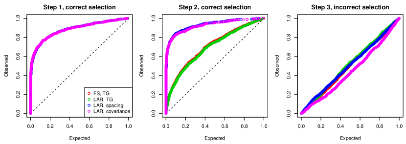
Figure 3: Simulated data with $n=50$, $p=100$, and two true active variables. Shown are p-values from the first 3 steps of FS and LAR, computed using the TG tests of Section 4, the spacing test of Section 5, and the covariance test of Lockhart et al. (2014), across 1000 repetitions (draws of $y$ from the simulation model).

6.2 Coverage of LAR conditional confidence intervals

In the same setup as the previous subsection, we computed conditional confidence intervals over the first 3 steps of LAR, at a 90% coverage level. Figure 4 shows these intervals across the first 100 repetitions. Each interval here is designed to cover the partial regression coefficient of a particular variable, in a population regression of the mean $\theta=X\beta^{*}$ on the variables in the current active set. These population coefficients are drawn as black dots, and the colors of the intervals reflect the identities of the variables being tested: red for variable 1, green for variable 2, and blue for all other variables. Circles around population coefficients indicate that these particular coefficients are not covered by their corresponding intervals. The miscoverage proportion is 12/100 in step 1, 11/100 in step 2, and 11/100 in step 3, all close to the nominal miscoverage level of 10%. An important remark: here we are counting marginal coverage of the intervals. Our theory actually further guarantees conditional coverage, for each model selection event; for example, among the red intervals at step 1, the miscoverage proportion is 7/52, and among green intervals, it is 5/47, both close to the nominal 10% level.

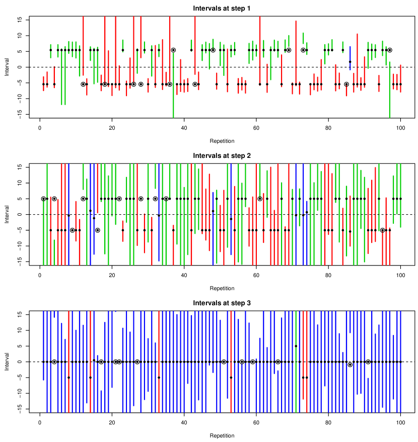
Figure 4: Using the same setup as in Figure 3, shown are 90% confidence intervals for the selections made over the first 3 steps of LAR, across 100 repetitions (draws of $y$ from the simulation model). The colors assigned to the intervals reflect the identities of the variables whose partial regression coefficients are being tested: red for variable 1, green for variable 2, and blue for all others. The black dots are the true population coefficients, and circles around these dots denote miscoverages. The upper confidence limits for some of the parameters exceed the range for the y-axes on the plots (especially at step 3).

6.3 Comparison to the max-$|t|$-test

The last two subsections demonstrated the unique properties of the exact TG tests for FS and LAR. For testing the significance of variables entered by FS, Buja & Brown (2014) proposed what they call the max-$|t|$-test. Here is a description. At the $k$th step of FS, where $A_{k-1}$ is the current active list (with $k-1$ active variables), let

$$t_{\max}(y)=\max_{j\notin A_{k-1}}\,\frac{|X_{j}^{T}P_{A_{k-1}}^{\perp}y|}{\sigma\|P_{A_{k-1}}^{\perp}X_{j}\|_{2}}.$$

As the distribution of $t_{\max}(y)$ is generally intractable, we simulate $\epsilon\sim N(0,\sigma^{2}I)$, and use this to estimate null probability that $t_{\max}(\epsilon)>t_{\max}(y)$, which forms our p-value.

We used the same setup as in the previous two subsections, but with an entirely null signal, i.e., we set the mean to be $\theta=X\beta^{*}=0$, in order to demonstrate the following point. As we step farther into the null regime (as we take more and more steps with FS), the max-$|t|$-test becomes increasingly conservative, whereas the exact TG test for FS continues to produce uniform p-values, as expected. The reason is that the TG test for FS at step $k$ properly accounts for all selection events up to and including step $k$, but the the max-$|t|$-test at step $k$ effectively ignores all selections occurring before this step, creating a conservative bias in the p-value. See Appendix A.5 for the plots.

7 Relationship to the covariance test

There is an interesting connection between the LAR spacing test and the covariance test of Lockhart et al. (2014). We first review the covariance test and then discuss this connection.

After $k$ steps of LAR, let $A_{k}$ denote the list of active variables and $s_{A_{k}}$ denote the sign list, the same notation as we have been using thus far. The covariance test provides a significance test for the $k$th step of LAR. More precisely, it assumes an underlying linear model $\theta=X\beta^{*}$, and tests the null hypothesis

$$H_{0}:\;\,A_{k-1}\supseteq\mathrm{supp}(\beta^{*}),$$

where $\mathrm{supp}(\beta^{*})$ denotes the support of set of $\beta^{*}$ (the true active set). In words, this tests simultaneously the significance of any variable entered at step $k$ and later.

Though its original definition is motivated from a difference in the (empirical) covariance between LAR fitted values, the covariance statistic can be written in an equivalent form that is suggestive of a connection to the spacing test. This form, at step $k$ of the LAR path, is

$$C_{k}=\omega_{k}^{2}\cdot\lambda_{k}(\lambda_{k}-\lambda_{k+1})/\sigma^{2},$$ (44)

where $\lambda_{k},\lambda_{k+1}$ are the LAR knots at steps $k$ and $k+1$ of the path, and $\omega_{k}$ is the weight in (41). (All proofs characterizing the null distribution of the covariance statistic in Lockhart et al. (2014) use this equivalent definition.) The main result (Theorem 3) in Lockhart et al. (2014) is that, under correlation restrictions on the predictors $X$ and other conditions, the covariance statistic (44) has a conservative $\mathrm{Exp}(1)$ limiting distribution under the null hypothesis. Roughly, they show that

$$\lim_{n,p\rightarrow\infty}\mathbb{P}_{A_{k-1}\supseteq\mathrm{supp}(\beta^{*})}\Big{(}C_{k}>t\,\Big{|}\,\hat{A}_{k}(y)=A_{k},\,\hat{s}_{A_{k}}(y)=s_{A_{k}}\Big{)}\leq e^{-t},$$

for all $t\geq 0$.

A surprising result, perhaps, is that the covariance test in (44) and the spacing test in (43) are asymptotically equivalent. The proof for this equivalence uses relatively straightforward calculations with Mills’ inequalities, and is deferred until Appendix A.6.

Theorem 3 (Asymptotic equivalence between spacing and covariance tests).

After a fixed number $k$ steps of LAR, the spacing p-value in (43) and the covariance statistic in (44) are asymptotically equivalent, in the following sense. Assume an asymptotic regime in which

$$\omega_{k}\lambda_{k+1}\overset{P}{\rightarrow}\infty,\;\;\;\text{and}$$

$$\omega_{k}^{2}\cdot\lambda_{k-1}(\lambda_{k-1}-\lambda_{k})\overset{P}{\rightarrow}\infty,$$

denoting convergence in probability. The spacing statistic, transformed by the inverse $\mathrm{Exp}(1)$ survival function, satisfies

$$-\log\Bigg{(}\frac{\Phi(\lambda_{k-1}\frac{\omega_{k}}{\sigma})-\Phi(\lambda_{k}\frac{\omega_{k}}{\sigma})}{\Phi(\lambda_{k-1}\frac{\omega_{k}}{\sigma})-\Phi(\lambda_{k+1}\frac{\omega_{k}}{\sigma})}\Bigg{)}=\frac{\omega_{k}^{2}}{\sigma^{2}}\lambda_{k}(\lambda_{k}-\lambda_{k+1})+o_{P}(1).$$

Said differently, the asymptotic p-value of the covariance statistic, under the $\mathrm{Exp}(1)$ limit, satisfies

$$\exp\bigg{(}-\frac{\omega_{k}^{2}}{\sigma^{2}}\lambda_{k}(\lambda_{k}-\lambda_{k+1})\bigg{)}=\Bigg{(}\frac{\Phi(\lambda_{k-1}\frac{\omega_{k}}{\sigma})-\Phi(\lambda_{k}\frac{\omega_{k}}{\sigma})}{\Phi(\lambda_{k-1}\frac{\omega_{k}}{\sigma})-\Phi(\lambda_{k+1}\frac{\omega_{k}}{\sigma})}\Bigg{)}(1+o_{P}(1)).$$

Above, we use $o_{P}(1)$ to denote terms converging to zero in probability.

Remark 7.

The asymptotic equivalence described in this theorem raises an interesting and unforeseen point about the one-sided nature of the covariance test. That is, the covariance statistic is seen to be asymptotically tied to the spacing p-value in (43), which, recall, we can interpret as testing the null $H_{0}:e_{k}^{T}X_{A_{k}}^{+}\theta=0$ against the one-sided alternative $H_{1}:{\mathrm{sign}}(e_{k}^{T}X_{A_{k}}^{+}y)\cdot e_{k}^{T}X_{A_{k}}^{+}\theta>0$. The covariance test in (44) is hence implicitly aligned to have power when the selected variable at the $k$th step has a sign that matches that of the projected population effect of this variable.

8 Discussion

In a regression model with Gaussian errors, we have presented a method for exact inference, conditional on a polyhedral constraint on the observations $y$. Since the FS, LAR, and lasso algorithms admit polyhedral representations for their model selection events, our framework produces exact p-values and confidence intervals post model selection for any of these adaptive regression procedures. One particularly special and simple case arises when we use our framework to test the significance of the projected regression coefficient, in the population, of the latest selected variable at a given step of LAR. This leads to the spacing test, which is asymptotically equivalent to the covariance test of Lockhart et al. (2014). An R language package selectiveInference, that implements the proposals in this paper, is freely available on the CRAN repository, as well as https://github.com/selective-inference/R-software. A Python implementation is also available, at https://github.com/selective-inference/Python-software.

Acknowledgements

We would like to thank Andreas Buja, Max Grazier G’Sell, Alessandro Rinaldo, and Larry Wasserman for helpful comments and discussion. We would also like to thank the editors and referees whose comments led to a complete overhaul of this paper! Richard Lockhart was supported by the Natural Sciences and Engineering Research Council of Canada; Jonathan Taylor was supported by NSF grant DMS 1208857 and AFOSR grant 113039; Ryan Tibshirani was supported by NSF grant DMS-1309174; Robert Tibshirani was supported by NSF grant DMS-9971405 and NIH grant N01-HV-28183.

Appendix A Proofs

A.1 Proof of Lemma 5

We first consider an alternative characterization for the optimality of a pair $(j_{k},s_{k})$ at an iteration $k$ of LAR. This characterization is already proved in Lemma 7 of Lockhart et al. (2014), and we present it here for reference.

Lemma 7 (Lemma 7 of Lockhart et al. 2014).

Consider an iteration $\ell$ of LAR, and define

$$\Sigma_{j,j^{\prime}}=c(j,s,A_{\ell-1},s_{A_{\ell-1}})^{T}c(j^{\prime},s^{\prime},A_{\ell-1},s_{A_{\ell-1}}),$$

for variables $j,j^{\prime}\notin A_{\ell-1}$ and signs $s,s^{\prime}$. (Note that $\Sigma_{j,j^{\prime}}$ actually depends on $s,s^{\prime}$, but we suppress this notationally for brevity.) Also define

$$S_{\ell}^{+}(j,s,\rho) =\Big{\{}(j^{\prime},s^{\prime}):j^{\prime}\notin A\cup\{j\},\;1-\Sigma_{j,j^{\prime}}/\Sigma_{jj}>0,\;c(j^{\prime},s^{\prime},A_{\ell-1},s_{A_{\ell-1}})^{T}y\leq\rho\Big{\}}$$

$$S_{\ell}^{-}(j,s,\rho) =\Big{\{}(j^{\prime},s^{\prime}):j^{\prime}\notin A\cup\{j\},\;1-\Sigma_{j,j^{\prime}}/\Sigma_{jj}<0,\;c(j^{\prime},s^{\prime},A_{\ell-1},s_{A_{\ell-1}})^{T}y\leq\rho\Big{\}}$$

$$S_{\ell}^{0}(j,s,\rho) =\Big{\{}(j^{\prime},s^{\prime}):j^{\prime}\notin A\cup\{j\},\;1-\Sigma_{j,j^{\prime}}/\Sigma_{jj}=0,\;c(j^{\prime},s^{\prime},A_{\ell-1},s_{A_{\ell-1}})^{T}y\leq\rho\Big{\}},$$

and

$$M_{\ell}^{+}(j,s,\rho)=\max_{(j^{\prime},s^{\prime})\in S_{\ell}^{+}(j,s,\rho)}\,\frac{c(j^{\prime},s^{\prime},A_{\ell-1},s_{A_{\ell-1}})^{T}y-(\Sigma_{j,j^{\prime}}/\Sigma_{j,j})\cdot c(j,s,A_{\ell-1},s_{A_{\ell-1}})^{T}y}{1-(\Sigma_{j,j^{\prime}}/\Sigma_{j,j})}$$

$$M_{\ell}^{-}(j,s,\rho)=\min_{(j^{\prime},s^{\prime})\in S_{\ell}^{-}(j,s,\rho)}\,\frac{c(j^{\prime},s^{\prime},A_{\ell-1},s_{A_{\ell-1}})^{T}y-(\Sigma_{j,j^{\prime}}/\Sigma_{j,j})\cdot c(j,s,A_{\ell-1},s_{A_{\ell-1}})^{T}y}{1-(\Sigma_{j,j^{\prime}}/\Sigma_{j,j})}$$

$$M_{\ell}^{0}(j,s,\rho)=\max_{(j^{\prime},s^{\prime})\in S_{\ell}^{0}(j,s,\rho)}\,c(j^{\prime},s^{\prime},A_{\ell-1},s_{A_{\ell-1}})^{T}y-(\Sigma_{j,j^{\prime}}/\Sigma_{j,j})\cdot c(j,s,A_{\ell-1},s_{A_{\ell-1}})^{T}y.$$

Then LAR selects $j_{\ell}$ and $s_{\ell}$ at iteration $\ell$ if and only if

$$c(j_{\ell},s_{\ell},A_{\ell-1},s_{A_{\ell-1}})^{T}y \leq\lambda_{\ell-1},$$ (45)

$$c(j_{\ell},s_{\ell},A_{\ell-1},s_{A_{\ell-1}})^{T}y \geq 0,$$ (46)

$$c(j_{\ell},s_{\ell},A_{\ell-1},s_{A_{\ell-1}})^{T}y \geq M_{\ell}^{+}(j_{\ell},s_{\ell},\lambda_{\ell-1}),$$ (47)

$$c(j_{\ell},s_{\ell},A_{\ell-1},s_{A_{\ell-1}})^{T}y \leq M_{\ell}^{-}(j_{\ell},s_{\ell},\lambda_{\ell-1}),$$ (48)

$$0 \geq M_{\ell}^{0}(j_{\ell},s_{\ell},\lambda_{\ell-1}).$$ (49)

Further, the triplet $(M_{\ell}^{+}(j_{\ell},s_{\ell}),M_{\ell}^{-}(j_{\ell},s_{\ell}),M_{\ell}^{0}(j_{\ell},s_{\ell}))$ is independent of $c(j_{\ell},s_{\ell},A_{\ell-1},s_{A_{\ell-1}})^{T}y$, for fixed $j_{\ell},s_{\ell}$.

We now recall another result of Lockhart et al. (2014) that is important in our context.

Lemma 8 (Lemma 9 of Lockhart et al. 2014).

At any iteration $\ell$ of LAR, we have

$$M_{\ell}^{+}(j_{\ell},s_{\ell},\lambda_{\ell-1})\leq c(j_{\ell+1},s_{\ell+1},A_{\ell},s_{A_{\ell}})^{T}y.$$

Finally, then, to build a list of constraints that are equivalent to the LAR algorithm selecting variables $A_{k}$ and signs $s_{A_{k}}$ through step $k$, we intersect conditions (45)–(49) from Lemma 7 over $\ell=1,\ldots k$. Notice that for each $\ell<k$, the inequality in (47) can be dropped, because it is implied by (45) and the result of Lemma 8,

$$c(j_{\ell},s_{\ell},A_{\ell-1},s_{A_{\ell-1}})^{T}y\geq c(j_{\ell+1},s_{\ell+1},A_{\ell},s_{A_{\ell}})^{T}y\geq M^{+}\Big{(}j_{\ell},s_{\ell},c(j_{\ell},s_{\ell},A_{\ell-1},s_{A_{\ell-1}})^{T}y\Big{)}.$$

This gives rise to conditions (34)–(37) in Lemma 5. The last condition (38) is needed to specify the sets $S_{\ell}$, $\ell=1,\ldots k$, and its construction follows that given in Section 4.2.

A.2 Proof of Lemma 6

One can see from its definition in Lemma 7 that $M_{k}^{+}$ is a maximum over linear functions of $y$ that are orthogonal to $\mathrm{col}(X_{A_{k}})$, the span of active variables. Hence, when $v\in\mathrm{col}(A_{k})$, we see that $M_{k}^{+}$ is a function of $(I-vv^{T}/\|v\|_{2}^{2})y$, certifying condition (39).

A.3 Proof of Theorem 1

As pointed out in Remark 3 after the theorem, we only need to prove that $\mathcal{V}^{\mathrm{lo}}=M_{k}^{+}$, $\mathcal{V}^{\mathrm{up}}=\lambda_{k-1}$, and $\|v\|_{2}=1/\omega_{k}$, and the result will then follow from Corollary 1 and the polyhedral inference lemmas from Section 3. Well, $\mathcal{V}^{\mathrm{lo}}$ and $\mathcal{V}^{\mathrm{up}}$ are the maximum and minimum of the quantities

$$\big{(}U_{j}-(\Gamma y)_{j}\big{)}\cdot\frac{\|v\|_{2}^{2}}{(\Gamma v)_{j}}+\lambda_{k},$$ (50)

over $j$ such that $(\Gamma v)_{j}>0$ and $(\Gamma v)_{j}<0$, respectively. In the above, we have used the fact that $v^{T}y=\lambda_{k}$, per its definition in (40).

Now, since $v$ proportional to $P_{A_{k-1}}^{\perp}X_{j_{k}}$, the first $k-1$ rows of $\Gamma$ are contained in $\mathrm{col}(X_{A_{k-1}})$, so $(\Gamma v)_{j}=0$ for $j=1,\ldots k-2$. For the $(k-1)$st row, we have $(\Gamma v)_{k-1}=-\|v\|_{2}^{2}$, and for the $k$th and $(k+1)$st row, we have $(\Gamma v)_{k}=(\Gamma v)_{k+1}=\|v\|_{2}^{2}$. The quantity $\mathcal{V}^{\mathrm{up}}$, therefore, is singularly defined in terms of the $(k-1)$st row. As $U_{k-1}=0$ and $(\Gamma y)_{k-1}=\lambda_{k-1}-\lambda_{k}$, we can see from (50) that $\mathcal{V}^{\mathrm{up}}=\lambda_{k-1}$. The quantity $\mathcal{V}^{\mathrm{lo}}$, meanwhile, is defined in by the $k$th and $(k+1)$st rows. As $U_{k}=0$, $U_{k+1}=M_{k}^{+}$, and $(\Gamma y)_{k}=(\Gamma y)_{k+1}=\lambda_{k}$, we can see from (50) that $\mathcal{V}^{\mathrm{lo}}=M_{k}^{+}$.

Lastly, the result $\|v\|_{2}=1/\omega_{k}$ can be seen by direct calculation, and is given in Lemma 10 of Lockhart et al. (2014).

A.4 Proof of Theorem 2

By Lemma 8 of Appendix A.1 (which recites Lemma 9 of Lockhart et al. (2014)) we know that $\lambda_{k+1}\geq M^{+}_{k}$. As the truncated Gaussian survival function is monotone increasing in its lower truncation limit, we have the relationship $\tilde{T}_{k}\geq T_{k}$, for the modified and original spacing statistics at step $k$. The fact that the latter is uniform under the null implies that the former is super-uniform under the null, establishing the result.

A.5 Plots for max-$|t|$-test comparison

Figure 5 displays the p-values from the TG test and the max-$|t|$-test over 6 steps of FS, and 1000 repetitions (draws of $y$ from an entirely null model, with mean zero). Both tests look good at step 1, but the max-$|t|$-test becomes more and more conservative for later steps. The reason is that TG test for FS conditions on all selection events up to and including that at step $k$—the same is true for the TG test for LAR, and its p-values would look exactly the same here. The max-$|t|$-test, however, does not do this. To be more explicit, the max-$|t|$-test at step 2 ignores the fact that the observed $t_{\max}(y)$ is the second largest value of the statistic in the data, and erroneously compares it to a reference distribution of largest $t_{\max}(\epsilon)$ values over a smaller set. This creates a conservative bias in the p-value. Remarkably, the exact TG test for FS (and LAR) is able carry out full conditioning on past selection events exactly.

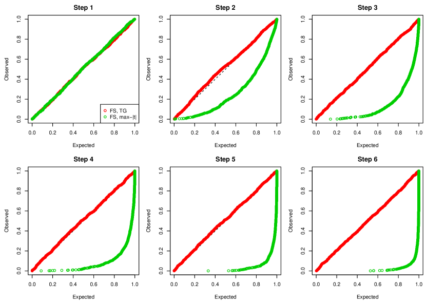
Figure 5: Using the same setup as in Figure 3, but with the mean being $\theta=X\beta^{*}=0$, shown are p-values from the first 6 steps of FS, using the TG test and the max-$|t|$-test, across 1000 repetitions (draws of $y$ from the simulation model).

A.6 Proof of Theorem 3

We begin with a helpful lemma based on Mills’ inequalities.

Lemma 9.

Suppose that $x,y\rightarrow\infty$ and $y(y-x)\rightarrow\infty$. Then, for $\Phi$ the standard normal CDF and $\phi$ the standard normal density,

$$\big{(}\Phi(y)-\Phi(x)\big{)}\cdot\frac{x}{\phi(x)}\rightarrow 1.$$

Proof.

Write

$$\Phi(y)-\Phi(x)=1-\Phi(x)-\big{(}1-\Phi(y)\big{)},$$

and apply Mills’ inequality to each of the survival terms individually, yielding

$$\frac{\phi(x)}{x}\frac{1}{1+1/x^{2}}-\frac{\phi(y)}{y}\leq\Phi(y)-\Phi(x)\leq\frac{\phi(x)}{x}-\frac{\phi(y)}{y}\frac{1}{1+1/y^{2}}.$$

Multiplying through by $x/\phi(x)$, and noting that

$$\frac{\phi(y)}{\phi(x)}=\exp(-(y+x)(y-x)/2)\leq\exp(-y(y-x)/2)\rightarrow 0,$$

we have established the result. ∎

Now consider

$$\tilde{T}_{k}=\frac{\Phi(\lambda_{k-1}\frac{\omega_{k}}{\sigma})-\Phi(\lambda_{k}\frac{\omega_{k}}{\sigma})}{\Phi(\lambda_{k-1}\frac{\omega_{k}}{\sigma})-\Phi(\lambda_{k+1}\frac{\omega_{k}}{\sigma})}.$$

We assume $\omega_{k}\lambda_{k+1}\overset{P}{\rightarrow}\infty$ (which implies the same of $\omega_{k}\lambda_{k}$, $\omega_{k}\lambda_{k-1}$), and $\omega_{k}^{2}\lambda_{k-1}(\lambda_{k-1}-\lambda_{k})\overset{P}{\rightarrow}\infty$ (which implies the same of $\omega_{k}^{2}\lambda_{k+1}(\lambda_{k-1}-\lambda_{k+1})$), hence we can use Lemma 9 to write

$$\tilde{T}_{k}=(1+o_{P}(1))\cdot\frac{\phi(\lambda_{k}\frac{\omega_{k}}{\sigma})}{\phi(\lambda_{k+1}\frac{\omega_{k}}{\sigma})}\cdot\frac{\lambda_{k+1}}{\lambda_{k}},$$

where $o_{P}(1)$ denotes a term converging to zero in probability. Thus

$$-\log(\tilde{T}_{k}) =\frac{\omega_{k}^{2}}{\sigma^{2}}\frac{\lambda_{k}^{2}-\lambda_{k+1}^{2}}{2}-\log\Big{(}\frac{\lambda_{k+1}}{\lambda_{k}}\Big{)}+o_{P}(1)$$

$$=\frac{\omega_{k}^{2}}{\sigma^{2}}\frac{\lambda_{k}(\lambda_{k}-\lambda_{k+1})}{2}+\frac{\omega_{k}^{2}}{\sigma^{2}}\frac{\lambda_{k+1}(\lambda_{k}-\lambda_{k+1})}{2}-\log\Big{(}\frac{\lambda_{k+1}}{\lambda_{k}}\Big{)}+o_{P}(1).$$

Using the assumption that $\lambda_{k}/\lambda_{k+1}\rightarrow 1$ in probability, this becomes

$$-\log(\tilde{T}_{k})=\frac{\omega_{k}^{2}}{\sigma^{2}}\lambda_{k}(\lambda_{k}-\lambda_{k+1})+o_{P}(1),$$

as desired.

References

• (1)
• Berk et al. (2013) Berk, R., Brown, L., Buja, A., Zhang, K. & Zhao, L. (2013), ‘Valid post-selection inference’, Annals of Statistics 41(2), 802–837.
• Buhlmann (2013) Buhlmann, P. (2013), ‘Statistical significance in high-dimensional linear models’, Bernoulli 19(4), 1212–1242.
• Buja & Brown (2014) Buja, A. & Brown, L. (2014), ‘Discussion: A significance test for the lasso’, Annals of Statistics 42(2), 509–517.
• Choi et al. (2014) Choi, Y., Taylor, J. & Tibshirani, R. (2014), Selecting the number of principal components: estimation of the true rank of a noisy matrix. arXiv: 1410.8260.
• Efron et al. (2004) Efron, B., Hastie, T., Johnstone, I. & Tibshirani, R. (2004), ‘Least angle regression’, Annals of Statistics 32(2), 407–499.
• Fithian et al. (2014) Fithian, W., Sun, D. & Taylor, J. (2014), Optimal inference after model selection. arXiv: 1410.2597.
• Fithian et al. (2015) Fithian, W., Taylor, J., Tibshirani, R. J. & Tibshirani, R. (2015), Adaptive sequential model selection. In preparation.
• G’Sell et al. (2015) G’Sell, M., Wager, S., Chouldechova, A. & Tibshirani, R. (2015), ‘Sequential selection procedures and false discovery rate control’, Journal of the Royal Statistical Society: Series B . To appear.
• Javanmard & Montanari (2013a) Javanmard, A. & Montanari, A. (2013a), Confidence intervals and hypothesis testing for high-dimensional regression. arXiv: 1306.3171.
• Javanmard & Montanari (2013b) Javanmard, A. & Montanari, A. (2013b), Hypothesis testing in high-dimensional regression under the gaussian random design model: Asymptotic theory. arXiv: 1301.4240.
• Lee et al. (2013) Lee, J., Sun, D., Sun, Y. & Taylor, J. (2013), Exact post-selection inference with the lasso. arXiv: 1311.6238.
• Lee & Taylor (2014) Lee, J. & Taylor, J. (2014), ‘Exact post model selection inference for marginal screening’, Advances in Neural Information Processing Systems 27.
• Lehmann & Romano (2005) Lehmann, E. & Romano, J. (2005), Testing Statistical Hypotheses, Springer, New York. Third edition.
• Lockhart et al. (2014) Lockhart, R., Taylor, J., Tibshirani, R. J. & Tibshirani, R. (2014), ‘A significance test for the lasso’, Annals of Statistics 42(2), 413–468.
• Loftus & Taylor (2014) Loftus, J. & Taylor, J. (2014), A significance test for forward stepwise model selection. arXiv: 1405.3920.
• Meinshausen & Buhlmann (2010) Meinshausen, N. & Buhlmann, P. (2010), ‘Stability selection’, Journal of the Royal Statistical Society: Series B 72(4), 417–473.
• Minnier et al. (2011) Minnier, J., Tian, L. & Cai, T. (2011), ‘A perturbation method for inference on regularized regression estimates’, Journal of the American Statistical Association 106(496), 1371–1382.
• Reid et al. (2014) Reid, S., Taylor, J. & Tibshirani, R. (2014), Post-selection point and interval estimation of signal sizes in Gaussian samples. arXiv: 1405.3340.
• Tibshirani (2013) Tibshirani, R. J. (2013), ‘The lasso problem and uniqueness’, Electronic Journal of Statistics 7, 1456–1490.
• van de Geer et al. (2014) van de Geer, S., Buhlmann, P., Ritov, Y. & Dezeure, R. (2014), ‘On asymptotically optimal confidence regions and tests for high-dimensional models’, Annals of Statistics 42(3), 1166–1201.
• Wasserman & Roeder (2009) Wasserman, L. & Roeder, K. (2009), ‘High-dimensional variable selection’, Annals of Statistics 37(5), 2178–2201.
• Zhang & Zhang (2014) Zhang, C.-H. & Zhang, S. (2014), ‘Confidence intervals for low dimensional parameters in high dimensional linear models’, Journal of the Royal Statistical Society: Series B 76(1), 217–242.