Jack–Laurent symmetric functions for special values of parameters

Abstract.

We consider the Jack–Laurent symmetric functions for special values of parameters $p_{0}=n+k^{-1}m,$ where $k$ is not rational and $m$ and $n$ are natural numbers. In general, the coefficients of such functions may have poles at these values of $p_{0}.$ The action of the corresponding algebra of quantum Calogero-Moser integrals $\mathcal{D}(k,p_{0})$ on the space of Laurent symmetric functions defines the decomposition into generalised eigenspaces. We construct a basis in each generalised eigenspace as certain linear combinations of the Jack–Laurent symmetric functions, which are regular at $p_{0}=n+k^{-1}m,$ and describe the action of $\mathcal{D}(k,p_{0})$ in these eigenspaces.

1. Introduction

The Jack symmetric functions $P_{\lambda}^{(k)}$ can be considered as one-parameter generalisation of Schur symmetric functions [5, 6] and play an important role in many areas of mathematics and theoretical physics. They can be also defined as the eigenfunctions of an infinite-dimensional version of the Calogero-Moser-Sutherland (CMS) operators [2].

In paper [7] we introduced and studied a Laurent version of Jack symmetric functions - Jack–Laurent symmetric functions $P^{(k,p_{0})}_{\alpha}$ as certain elements of $\Lambda^{\pm}$ labelled by bipartitions $\alpha=(\lambda,\mu)$, which are pairs of the usual partitions $\lambda$ and $\mu.$ Here $\Lambda^{\pm}$ is freely generated by $p_{a}$ with $a\in\mathbb{Z}\setminus\{0\}$ being both positive and negative. The variable $p_{0}$ plays a special role and is considered as an additional parameter. The usual Jack symmetric functions $P_{\lambda}^{(k)}$ are particular cases of $P^{(k,p_{0})}_{\alpha}$ corresponding to empty second partition $\mu.$ The simplest example of Jack–Laurent symmetric function corresponding to two one-box Young diagrams is given by

$$P^{(k,p_{0})}_{1,1}=p_{1}p_{-1}-\frac{p_{0}}{1+k-kp_{0}}.$$

We proved the existence of $P^{(k,p_{0})}_{\alpha}$ for all $k\notin\mathbb{Q}$ and $p_{0}\neq n+k^{-1}m,\,m,n\in\mathbb{Z}_{>0}$ (see Theorem 4.1 in [7]). The coefficients of $P^{(k,p_{0})}_{\alpha}$ as functions of $p_{0}$ are rational and may have poles at $p_{0}=n+k^{-1}m$ with natural $m,n,$ so the corresponding Jack–Laurent symmetric function may not exist (as one can see in the example above). This is related to the fact that the spectrum of the algebra of the corresponding quantum CMS integrals $\mathcal{D}(k,p_{0})$ is not simple, which leads to the decomposition of $\Lambda^{\pm}$ into generalised eigenspaces.

In this paper we fix a non-rational value of $k$ and study the analytic properties of Jack–Laurent symmetric functions as functions of $p_{0}$ at the special values $p_{0}=n+k^{-1}m$. The main result is the construction of a basis in each generalised eigenspace of $\mathcal{D}(k,p_{0})$ as certain linear combinations of the Jack–Laurent symmetric functions, which are regular at $p_{0}=n+k^{-1}m$.

The structure of the paper is as follows. In the next section we introduce the equivalence relation on the set of bipartitions induced by the action of the algebra $\mathcal{D}(k,p_{0})$ and study it in detail. In particular, we show that each equivalence class $E$ consists of $2^{r}$ elements, which can be explicitly described in terms of geometry of the corresponding Young diagrams (see Fig. 1 below).

In the third section we construct the linear combinations of Jack–Laurent symmetric functions

$$Q^{(k,p_{0})}_{\alpha}=\sum_{\beta\in E,\,\,\beta\subset\alpha}a_{\beta\alpha}(k,p_{0})P^{(k,p_{0})}_{\beta},$$

which are regular at $p_{0}=n+k^{-1}m$ and give a basis in the corresponding generalised eigenspace. Here $E$ is the equivalence class of bipartition $\alpha$ and $a_{\beta\alpha}(k,p_{0})$ are some rational functions of $p_{0}$ with poles at $p_{0}=n+k^{-1}m$ of known order (see Theorem 3.6 below). As a corollary we describe the order of the pole of $P^{(k,p_{0})}_{\alpha}$ at $p_{0}=n+k^{-1}m$ in terms of the geometry of the corresponding bipartition $\alpha.$ We are using the technique similar to the translation functors in the representation theory [1, 8] and based on the Pieri formula for Jack–Laurent symmetric functions derived in [7].

In the last section we describe the action of the algebra $\mathcal{D}(k,p_{0})$ with $p_{0}=n+k^{-1}m$ in each generalised eigenspace $V_{E}$. More precisely, we show that provided $k$ is non-algebraic the image of $\mathcal{D}(k,p_{0})$ in $End\,V_{E}$ is isomorphic to the tensor product of $r$ copies of dual numbers $\mathfrak{A}_{r}=\mathbb{C}[\varepsilon]^{\otimes r}$, $\varepsilon^{2}=0$ and the corresponding action of $\mathfrak{A}_{r}$ in $V_{E}$ is the regular representation of $\mathfrak{A}_{r}$.

2. Equivalence relation

We start with the following result from our paper [7] about the quantum CMS integrals at infinity.

Let us assume at the beginning that $k$ is not rational and $p_{0}\neq n+k^{-1}m,\,m,n\in\mathbb{Z}_{>0}$ and consider the corresponding Jack-Laurent symmetric function $P^{(k,p_{0})}_{\alpha}$ indexed by bipartition $\alpha=(\lambda,\mu)$ (see [7] for the precise definition). We will use the standard representation of the partitions as Young diagrams [6].

Theorem 2.1.

[7] There exist quantum CMS integrals $\mathcal{B}^{(r)}:\Lambda^{\pm}\rightarrow\Lambda^{\pm}$ polynomially depending on $p_{0}$ such that

$$\mathcal{B}^{(r)}P^{(k,p_{0})}_{\alpha}=b_{r}(\alpha,k,p_{0})P^{(k,p_{0})}_{\alpha},$$ (1)

where

$$b_{r}(\alpha,k,p_{0})=\left(\sum_{x\in\lambda}c(x,0)^{r-1}+(-1)^{r}\sum_{x\in\mu}c(x,1+k-kp_{0})^{r-1}\right)$$ (2)

and the content $c(x,a)$ of the box $x=(ij)$ is defined by

$$c(x,a)=(j-1)+k(i-1)+a.$$

The algebra of CMS integrals $\mathcal{D}(k,p_{0})$ is generated by these operators.

Let us introduce the following equivalence relation $\mathcal{E}$ on bipartitions, depending on parameters $k,p_{0}.$ We say that $\alpha=(\lambda,\mu)$ is $\mathcal{E}$-equivalent to $\tilde{\alpha}=(\tilde{\lambda},\tilde{\mu})$ if and only if for all $r\geq 1$ we have

$$b_{r}(\alpha,k,p_{0})=b_{r}(\tilde{\alpha},k,p_{0}),$$

or, more explicitly,

$$\sum_{x\in\lambda}c(x,0)^{r-1}+(-1)^{r}\sum_{y\in\mu}c(y,1+k-kp_{0})^{r-1}$$ (3)

$$=\sum_{x\in\tilde{\lambda}}c(x,0)^{r-1}+(-1)^{r}\sum_{y\in\tilde{\mu}}c(y,1+k-kp_{0})^{r-1}.$$

If parameters $k,p_{0}$ are non-special, then this equivalence relation is trivial. More precisely, we have the following result [7].

Proposition 2.2.

If $k$ is not rational and $p_{0}\neq n+k^{-1}m,\,m,n\in\mathbb{Z}_{>0},$ then $\alpha$ is $\mathcal{E}$-equivalent to $\tilde{\alpha}$ if and only if $\alpha=\tilde{\alpha}.$

Proof.

If (3) is true for all $r\geq 1$ then the sequences

$$(c(x,0),-c(y,1+k-kp_{0}))_{x\in\lambda,y\in\tilde{\mu}},\quad(c(x,0),-c(y,1+k-kp_{0}))_{x\in\tilde{\lambda},y\in\mu}$$

coincide up to a permutation. Therefore we have for every $x\in\lambda$ two possibilities: $c(x,0)=c(\tilde{x},0)$ for some $\tilde{x}\in\tilde{\lambda}$, or $c(x,0)=-c(\tilde{y},1+k-kp_{0})$ for some $\tilde{y}\in\mu$. In the first case we have for $x=(ij),\,\tilde{x}=(\tilde{i}\tilde{j})$ the relation $j-\tilde{j}+k(i-\tilde{i})=0$, so $j=\tilde{j},\,i=\tilde{i}$ since $k$ is not rational.

In the second case we have for $\tilde{y}=(\tilde{i}\tilde{j})$ that

$$kp_{0}=j+\tilde{j}-1+k(i+\tilde{i}-1),$$ (4)

which contradicts to our assumption, since both $j+\tilde{j}-1$ and $i+\tilde{i}-1$ are positive integers. ∎

Consider now the case of special values of parameters when

$$p_{0}=n+k^{-1}m$$

for some $n,m\in\mathbb{Z}_{>0},$ still assuming that $k$ is not rational. Denote by $\pi(n,m)$ the rectangular Young diagram of size $n\times m$ and the corresponding bipartition $\pi=(\pi(n,m),\pi(n,m))$. Define the central symmetry transformation $\theta$ acting on $(ij)\in\pi(n,m)$ by

$$\theta(ij)=(n-i+1,m-j+1).$$

Inclusion of the Young diagrams induces the following partial order on bipartitions. We say that $\alpha\subset\tilde{\alpha}$ if and only if $\lambda\subset\tilde{\lambda}$ and $\mu\subset\tilde{\mu}$, where the Young diagrams are understood as the subsets of the plane. We will use the same convention for all set-theoretical operations for bipartitions.

Proposition 2.3.

Bipartition $\alpha=(\lambda,\mu)$ is $\mathcal{E}$-equivalent to $\tilde{\alpha}=(\tilde{\lambda},\tilde{\mu})$ if and only if

$$\alpha\setminus\pi=\tilde{\alpha}\setminus\pi$$ (5)

and

$$\theta(\lambda\setminus\tilde{\lambda})=\mu\setminus\tilde{\mu},\quad\theta(\tilde{\lambda}\setminus\lambda)=\tilde{\mu}\setminus\mu.$$ (6)

Proof.

We will use the notations from the proof of the previous proposition. If $\alpha$ is equivalent to $\tilde{\alpha},$ then for any $x=(ij)\in\lambda\setminus\pi(n,m)$ there is only the first possibility and therefore $x\in\tilde{\lambda}\setminus\pi(n,m).$ Thus $\lambda\setminus\pi(n,m)\subset\tilde{\lambda}\setminus\pi(n,m),$ and by symmetry $\lambda\setminus\pi(n,m)=\tilde{\lambda}\setminus\pi(n,m).$ Similarly we have $\mu\setminus\pi(n,m)=\tilde{\mu}\setminus\pi(n,m)$ and (5).

From (5) it follows that $\lambda\setminus\tilde{\lambda}$ is contained in $\pi(n,m).$ For $x=(ij)\in\lambda\setminus\tilde{\lambda}$ there exists only second possibility, which means that there exists $\tilde{y}=(\tilde{i}\tilde{j})\in\mu$ such that $j+\tilde{j}-1+k(i+\tilde{i}-1)=kp_{0}=n+km.$ Since $k$ is not rational, this implies that

$$j+\tilde{j}-1=n,\quad i+\tilde{i}-1=m,$$

which means that $\theta(x)\in\mu\setminus\tilde{\mu}.$ Similarly we have $\theta(\mu\setminus\tilde{\mu})\subset\lambda\setminus\tilde{\lambda}.$ Since $\theta$ is an involution, this implies

$$\theta(\lambda\setminus\tilde{\lambda})=\mu\setminus\tilde{\mu}.$$

By symmetry we have $\theta(\tilde{\lambda}\setminus\lambda)=\tilde{\mu}\setminus\mu.$

Conversely, assume that we have the relations (5), (6). We have to show that the sequences

$$(c(x,0),-c(y,1+k-kp_{0}))_{x\in\lambda,y\in\tilde{\mu}},\quad(c(x,0),-c(y,1+k-kp_{0}))_{x\in\tilde{\lambda},y\in\mu}$$

coincide up to a permutation. We have the disjoint unions

$$\lambda=(\lambda\setminus\pi(n,m))\cup(\lambda\setminus\tilde{\lambda})\cup(\lambda\cap\tilde{\lambda}\cap\pi(n,m)),$$

$$\tilde{\mu}=(\tilde{\mu}\setminus\pi(n,m))\cup(\tilde{\mu}\setminus\mu)\cup(\tilde{\mu}\cap\mu\cap\pi(n,m)),$$

$$\tilde{\lambda}=(\tilde{\lambda}\setminus\pi(n,m))\cup(\tilde{\lambda}\setminus\lambda)\cup(\lambda\cap\tilde{\lambda}\cap\pi(n,m)),$$

$$\mu=(\mu\setminus\pi(n,m))\cup(\mu\setminus\tilde{\mu})\cup(\mu\cap\tilde{\mu}\cap\pi(n,m)).$$

Using this, the relations (5), (6) and the identity

$$c(\theta(x),1+k-kp_{0})=(m+kn-kp_{0})-c(x,0),\,\,x\in\pi(n,m)$$ (7)

we can identify the corresponding contributions in these sequences and have the result. ∎

Consider the set $\mathcal{P}_{n,m}$ of bipartitions $\alpha\subset\pi=(\pi(n,m),\pi(n,m)).$ For such partitions the equivalence relation can be described in the following simple way. Introduce the involution $\omega:\mathcal{P}_{n,m}\rightarrow\mathcal{P}_{n,m}$ such that for $\alpha=(\lambda,\mu)$

$$\omega(\alpha)=(\lambda,\pi(n,m)\setminus\theta(\mu)).$$ (8)

Introduce now another equivalence relation $\mathcal{R}$ on bipartitions. We say that $\alpha=(\lambda,\mu)$ is $\mathcal{R}$-equivalent $\tilde{\alpha}=(\tilde{\lambda},\tilde{\mu})$ if

$$\lambda\cap\mu=\tilde{\lambda}\cap\tilde{\mu},\,\,\,\lambda\cup\mu=\tilde{\lambda}\cup\tilde{\mu}.$$ (9)

Theorem 2.4.

On the set $\mathcal{P}_{n,m}$ the involution (8) transforms the equivalence relation $\mathcal{E}$ into $\mathcal{R}.$

Proof.

Let $\alpha=(\lambda,\mu)$ be $\mathcal{E}$-equivalent to $\tilde{\alpha}=(\tilde{\lambda},\tilde{\mu}).$ It is enough to prove that

$$\lambda\cup(\pi(n,m)\setminus\theta(\mu))=\tilde{\lambda}\cup(\pi(n,m)\setminus\theta(\tilde{\mu}))$$ (10)

and

$$\lambda\cap(\pi(n,m)\setminus\theta(\mu))=\tilde{\lambda}\cap(\pi(n,m)\setminus\theta(\tilde{\mu})).$$ (11)

Let’s prove (11). Let $x\in\lambda\cap(\pi(n,m)\setminus\theta(\mu)),$ then $x\in\lambda$ and $x\notin\theta(\mu).$

Assume that $x\notin\tilde{\lambda}$, then from (6) it follows that $\theta(x)\in\mu$ and thus $x\in\theta(\mu).$ Contradiction means that $x\in\tilde{\lambda}.$

Assume now that $x\notin\pi(n,m)\setminus\theta(\tilde{\mu}),$ which means that $x\in\theta(\tilde{\mu}).$ Since $x\notin\theta(\mu)$ we have $x\in\theta(\tilde{\mu}\setminus\mu).$ Using the second part of (6) we see that $x\in\tilde{\lambda}\setminus\lambda$ and hence $x\notin\lambda$, which is a contradiction. Now (11) follows from the symmetry between $\alpha$ and $\tilde{\alpha}.$ The proof of (10) is similar.

This proves that $\mathcal{E}$-equivalence implies $\mathcal{R}$-equivalence for $\omega$-transformed bipartitions. The converse claim can be proved in a similar way. ∎

This can be used to describe the structure of $\mathcal{E}$-equivalence classes of bipartitions from $\mathcal{P}_{n,m}$.

Theorem 2.5.

Let $\alpha\in\mathcal{P}_{n,m}$ and $E$ be its $\mathcal{E}$-equivalence class. Then the following holds true:

$1)$ $E\subset\mathcal{P}_{n,m}.$

$2)$ $E$ contains the minimal and maximal bipartitions $\alpha_{m},\,\alpha_{M}$ such that

$$\alpha_{m}\subset\alpha\subset\alpha_{M}$$

for any bipartition $\alpha\in E$. They can be characterised by the properties $\lambda\cap\theta(\mu)=\emptyset$ and by $\lambda\cup\theta(\mu)=\pi(n,m)$ respectively.

$3)$ Let $\alpha_{m}=(\lambda_{m},\mu_{m}),\,\alpha_{M}=(\lambda_{M},\mu_{M})$ and

$$\lambda_{M}\setminus\lambda_{m}=\nu_{1}\cup\nu_{2}\cup\dots\cup\nu_{r},\,\,\mu_{M}\setminus\mu_{m}=\tau_{1}\cup\tau_{2}\cup\dots\cup\tau_{s}$$ (12)

be the decomposition of the corresponding skew diagrams into connected components. Then $\nu_{i},\tau_{j}\subset\pi(n,m)$, $r=s$ and, after a reordering,

$$\theta(\nu_{i})=\tau_{i},\,\,i=1,2,\dots,r.$$

$4)$ Every element $\alpha$ from $E$ can be represented uniquely in the form

$$\alpha=\alpha_{m}\cup(\nu_{a_{1}},\tau_{a_{1}})\cup(\nu_{a_{2}},\tau_{a_{2}})\cup\dots\cup(\nu_{a_{l}},\tau_{a_{l}}),$$ (13)

where $\{a_{1},\,a_{2},\dots,a_{l}\}$ is a subset of $\{1,\,2,\dots,r\}.$ Any set of this form is a bipartition from $E,$ so the equivalence class $E$ contains $2^{r}$ elements.

Proof.

The first part follows immediately from (5). Applying the involution $\omega$ and the previous theorem we have the remaining claims using simple geometric analysis of the corresponding Young diagrams (see Fig. 1). ∎

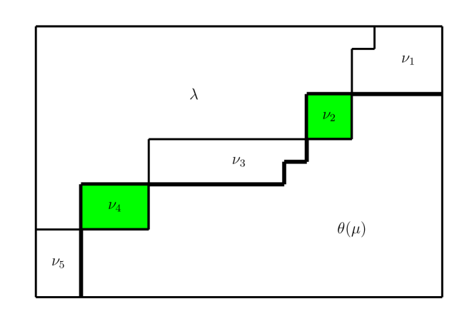
Figure 1. Intersection of $\lambda$ and $\theta(\mu)$ (shaded) in the rectangle $\pi((n,m)$ and the corresponding connected components $\nu_{i}.$ The boundary of $\theta(\mu)$ is shown in bold.

To describe $\mathcal{E}$-equivalence class for general bipartition $\alpha=(\lambda,\mu)$ denote by $\alpha_{\pi}$ the bipartition $\alpha_{\pi}=\alpha\cap\pi=(\lambda_{\pi},\mu_{\pi}):$

$$(\lambda_{\pi},\mu_{\pi})=(\lambda\cap\pi(n,m),\mu\cap\pi(n,m)).$$

Corollary 2.6.

Let $E(\alpha_{\pi})$ be the $\mathcal{E}$-equivalence class of $\alpha_{\pi}$. Then $\mathcal{E}$-equivalence class of $\alpha$ can be described as

$$E(\alpha)=\{\gamma=\beta\cup(\alpha\setminus\pi)\in\mathcal{P}\times\mathcal{P}\mid\beta\in E(\alpha_{\pi})\}.$$

$E(\alpha)$ contains the minimal and maximal bipartitions $\alpha_{m},\,\alpha_{M}$ such that

$$\alpha_{m}\subset\alpha\subset\alpha_{M}$$

with parts $3)$ and $4)$ of theorem 2.5 remaining valid for any bipartition $\alpha.$

Note that $E(\alpha)\cap\mathcal{P}_{n,m}\subset E(\alpha_{\pi})$ in general does not coincide with $E(\alpha_{\pi}).$

3. Translation functors and regular basis

In [7] we have introduced the Jack-Laurent symmetric functions $P_{\alpha}=P^{(k,p_{0})}_{\alpha}\in\Lambda^{\pm}$ indexed by bipartition $\alpha=(\lambda,\mu).$ As we have shown they are well defined provided $k$ is not rational and $p_{0}\neq n+k^{-1}m$ with $n,m\in\mathbb{Z}_{>0}.$ Equivalently, we can consider $P_{\alpha}$ as elements of $\Lambda^{\pm}_{p_{0}}=\Lambda^{\pm}\otimes\mathbb{C}(p_{0})$, where $\mathbb{C}(p_{0})$ is the field of rational functions of $p_{0}.$

Now we are going to study what happens when $p_{0}=n+k^{-1}m$ assuming that $k,n,m$ are fixed with $k$ not rational and $n,m\in\mathbb{Z}_{>0}.$ Then $P_{\alpha}^{(k,p_{0})}$ as functions of $p_{0}$ may have pole at $p_{0}=n+k^{-1}m$ depending on the choice of bipartition $\alpha.$

The aim of this section is to construct a basis in $\Lambda^{\pm}$ which is regular at $p_{0}=n+k^{-1}m$. More precisely, we will define the Laurent symmetric functions $Q_{\alpha}=Q^{(k,p_{0})}_{\alpha}\in\Lambda^{\pm}$, which are regular at $p_{0}=n+k^{-1}m$, such that for any $\alpha$

$$Q_{\alpha}=\sum_{\beta\in E(\alpha),\,\beta\subset\alpha}a_{\beta\alpha}P_{\beta}$$

with some coefficients $a_{\beta\alpha}=a_{\beta\alpha}(k,p_{0})$ which are rational functions of $p_{0}.$

In order to do this we are going to produce some family of linear transformations $\mathcal{F}_{E,F}$ acting on $\Lambda^{\pm}_{p_{0}}$ which are similar to the translation functors in the representation theory [1, 8].

Let $E$ be an $\mathcal{E}$-equivalence class of bipartitions and $V_{E}\subset\Lambda^{\pm}_{p_{0}}$ be the linear span over $\mathbb{C}(p_{0})$ of $P_{\alpha}$ with $\alpha\in E.$ We have the decomposition of vector spaces over $\mathbb{C}(p_{0})$

$$\Lambda^{\pm}_{p_{0}}=\bigoplus_{E}V_{E},$$

where the sum is taken over all $\mathcal{E}$-equivalence classes of bipartitions.

Denote by $Pr_{E}$ the projector onto the subspace $V_{E}$ with respect to this decomposition and define for any $\mathcal{E}$-equivalence classes $E$ and $F$ the linear map

$$\mathcal{F}_{E,F}(f):=Pr_{F}(p_{1}f),\,f\in V_{E}.$$ (14)

The next result is quite simple but very important.

Proposition 3.1.

Let $f\in V_{E}$ and suppose that $f$ has no pole at $p_{0}=n+k^{-1}m$. Then for any $\mathcal{E}$-equivalence class $F$ the function $\mathcal{F}_{E,F}(f)$ also has no pole at $p_{0}=n+k^{-1}m$.

Proof.

We have

$$p_{1}V_{E}\subset V_{F}\oplus V_{E_{1}}\oplus\dots\oplus V_{E_{L}}$$ (15)

where $F,\,E_{1},\dots,E_{L}$ are different classes of equivalence. First we will construct linear operator $\mathcal{C}_{1}$ which polynomially depends on CMS integrals $\mathcal{B}^{(r)}$ with coefficients having no poles at $p_{0}=n+k^{-1}m$ and such that

$$\mathcal{C}_{1}(V_{E_{1}})=0,\,\,\mathcal{C}_{1}(v)=v,\,\,v\in V_{F}$$

Let $\alpha_{1},\dots,\alpha_{N}$ be all bipartitions in $F$ and $\beta_{1},\dots,\beta_{M}$ all bipartitions in $E_{1}$. Then by definition of the equivalence classes there is $r_{1}\in\mathbb{Z}_{>0}$ such that

$$b_{r_{1}}(\alpha_{1},k,p_{0})\neq b_{r_{1}}(\beta_{j},k,p_{0}),\,\,\,j=1,\dots,M$$

when $p_{0}=n+k^{-1}m.$ Let

$$f_{1}(t)=\prod_{j=1}^{M}(t-b_{r_{1}}(\beta_{j},k,p_{0})),$$

then operator $\mathcal{D}_{1}=f_{1}(\mathcal{B}^{(r_{1})})$, where $\mathcal{B}^{(r)}$ are the CMS integrals from Theorem 2.1, acts as zero in $V_{E_{1}}$ and in $V_{F}$ as a diagonal operator

$$\mathcal{D}_{1}P_{\alpha_{i}}=g_{1}(\alpha_{i},k,p_{0})P_{\alpha_{i}},\,\,i=1,\dots,N,$$

where $g_{1}(\alpha_{i},k,p_{0})=f_{1}(b_{r_{1}}(\alpha_{i},k,p_{0})).$ Now having in mind Cayley-Hamilton theorem we can define

$$\mathcal{C}_{1}=(-1)^{N+1}\frac{1}{\sigma_{N}}\left(\mathcal{D}_{1}^{N}-\sigma_{1}\mathcal{D}_{1}^{N-1}+\dots+(-1)^{N-1}\sigma_{N-1}\mathcal{D}_{1}\right)$$

where $\sigma_{1},\dots,\sigma_{N}$ stand for the elementary symmetric polynomials in

$$g_{1}(\alpha_{1},k,p_{0}),\,\dots\,,g_{1}(\alpha_{N},k,p_{0}).$$

From our assumptions we see that $\sigma_{N}=g_{1}(\alpha_{1},k,p_{0})\dots g_{1}(\alpha_{N},k,p_{0})\neq 0$ when $p_{0}=k^{-1}n+m.$ We see that $\mathcal{C}_{1}(V_{E_{1}})=0$ and by the Cayley-Hamilton theorem $\mathcal{C}_{1}$ acts as the identity in $V_{F}$.

In the same way we can construct operators $\mathcal{C}_{2},\dots\mathcal{C}_{L}$ and define

$$\mathcal{C}=\mathcal{C}_{1}\mathcal{C}_{2}\dots\mathcal{C}_{L}.$$

Let $p_{1}f=g+g_{1}+\dots+g_{L}$ be the decomposition according to (15). Applying to both sides of this equality the operator $\mathcal{C}$ we get

$$\mathcal{C}(p_{1}f)=g=Pr_{F}(p_{1}f).$$

But, since $\mathcal{B}^{(r)}$ are polynomial in $p_{0},$ $\mathcal{C}$ is a differential operator with coefficients that have no poles at $p_{0}=n+k^{-1}m$, so both sides must be regular at this point. ∎

The following definition is motivated by the Pieri formula for Jack–Laurent symmetric functions [7]. Let $\alpha=(\lambda,\mu)\in\mathcal{P}_{n,m}$ be a bipartition inside $\pi.$

For any box $x\in\pi(n,m)$ define the set of bipartitions $S_{x}(\alpha)$ as

$$S_{x}(\alpha)=\{(\lambda\cup x,\mu),\,(\lambda,\mu\setminus\theta(x))\}$$

assuming that $x\notin\lambda$ and $\lambda\cup x$ is a Young diagram, and that $\theta(x)\in\mu$ and $\mu\setminus\theta(x)$ is a Young diagram (otherwise the corresponding element is dropped from the set).

Let us denote by $X(\alpha)$ the set of all bipartitions in the right hand side of the Pieri formula (see formula (56) from [7]): $X(\alpha)$ is the set of all bipartions $\beta=(\tilde{\lambda},\tilde{\mu})$ such that $\alpha$ can be obtained from $\beta$ by deleting a box from $\tilde{\lambda}$ or adding a box to $\tilde{\mu}.$

Proposition 3.2.

Let $E$ be an $\mathcal{E}$-equivalence class and suppose that there is $\alpha\in E$ such that $S_{x}(\alpha)$ is not empty. Then there exists a unique $\mathcal{E}$-equivalence class $E_{x}$ different from $E$ such that for any $\alpha\in E$

$$X(\alpha)\cap E_{x}=S_{x}(\alpha).$$

Proof.

Let us prove first that if $\alpha$ is $\mathcal{E}$-equivalent to $\tilde{\alpha}$ then $S_{x}(\alpha)$ and $S_{x}(\tilde{\alpha})$ belong to the same $\mathcal{E}$-equivalence class. Applying the involution $\omega$ we reduce this to the following statement. Let $\omega(\alpha)=(\lambda,\mu),\omega(\tilde{\alpha})=(\tilde{\lambda},\tilde{\mu})$ and

$$\lambda\cup\mu=\tilde{\lambda}\cup\tilde{\mu},\,\lambda\cap\mu=\tilde{\lambda}\cap\tilde{\mu}.$$

Without loss of generality we can assume that the box $x$ can be added to $\lambda$ and $\tilde{\lambda}$. We need to prove that

$$(\lambda\cup x)\cup\mu=(\tilde{\lambda}\cup x)\cup\tilde{\mu},\,\,\,(\lambda\cup x)\cap\mu=(\tilde{\lambda}\cup x)\cap\tilde{\mu}.$$

The first equality is obvious. To prove the second consider two cases: $x\notin\mu$ and $x\in\mu.$

If $x\notin\mu$ then $x\notin\lambda\cup\mu=\tilde{\lambda}\cup\tilde{\mu},$ hence $x\notin\tilde{\mu},$ which implies that $(\lambda\cup x)\cap\mu=(\tilde{\lambda}\cup x)\cap\tilde{\mu}.$

If $x\in\mu$ then $x\in\lambda\cup\mu=\tilde{\lambda}\cup\tilde{\mu},$ and hence $x\in\tilde{\mu}.$ Therefore

$$(\lambda\cup x)\cap\mu=\lambda\cap\mu=\tilde{\lambda}\cap\tilde{\mu}=(\tilde{\lambda}\cup x)\cap\tilde{\mu}.$$

Hence there exists a unique equivalence class $E_{x}$ containing the union of $S_{x}(\alpha),\,\alpha\in E.$ The relation $X(\alpha)\cap E_{x}=S_{x}(\alpha)$ is easy to check.

We only left to prove that these equivalence classes $E$ and $E(x)$ are different. Suppose that $(\lambda,\mu)$ and $(\lambda\cup x,\mu)$ are $\mathcal{R}$-equivalent. Then we have

$$\lambda\cup\mu=\lambda\cup x\cup\mu,\,\,\lambda\cap\mu=(\lambda\cup x)\cap\mu,$$

implying that $x\in\lambda,$ which is a contradiction. ∎

For any box $x\in\pi(n,m)$ define now the set of bipartitions $S^{x}(\alpha)$ as

$$S^{x}(\alpha)=\{(\lambda\setminus x,\mu),\,(\lambda,\mu\cup\theta(x))\}.$$

In the same way as in proposition 3.2 it can be proven that there exists a unique $\mathcal{E}$-equivalence class $E^{x}$, which contains $S^{x}(\alpha)$ for any $\alpha\in E.$

Let $x\in\pi(n,m)$. Denote by $\mathcal{F}_{x}$ the linear transformation defined by

$$\mathcal{F}_{x}=\mathcal{F}_{E,E_{x}}.$$

The following proposition is based on the Pieri formula for Jack-Laurent symmetric functions [7]. Introduce the following functions for bipartition $\alpha=(\lambda,\mu)$ and box $x=(ij)$:

$$U(x,\alpha;p_{0})=U_{1}(x,\alpha)U_{2}(x,\alpha;p_{0})U_{3}(x,\alpha;p_{0}),$$ (16)

$$U_{1}(x,\alpha)=\prod_{r=i+1}^{l(\mu)}\frac{c_{\mu}(jr,1+k)c_{\mu}(jr,-k)}{c_{\mu}(jr,1)c_{\mu}(jr,0)},$$ (17)

$$U_{2}(x,\alpha;p_{0})=\prod_{r=1}^{l(\lambda)}\frac{c_{\alpha}(jr,-1-k(p_{0}+2))c_{\alpha}(jr,-kp_{0})}{c_{\alpha}(jr,-1-k(p_{0}+1))c_{\alpha}(jr,-k(p_{0}+1))},$$ (18)

$$U_{3}(x,\alpha;p_{0})=\frac{(j-1+k(l(\lambda)+\mu^{\prime}_{j}-p_{0}-1))(j+k(\mu^{\prime}_{j}-l(\mu)))}{(j+k(l(\lambda)+\mu^{\prime}_{j}-p_{0}))(j-1+k(\mu^{\prime}_{j}-l(\mu)-1))},$$ (19)

where

$$c_{\lambda}(jr,a)=\lambda_{r}-j-k(\lambda^{\prime}_{j}-r)+a,\;\;$$

$$c_{\alpha}(jr,a)=\lambda_{r}+j+k(\mu^{\prime}_{j}+r)+a,$$

and $\lambda^{\prime}$ as before is the Young diagram conjugated (transposed) to $\lambda$.

Proposition 3.3.

The action of $\mathcal{F}_{x}$ on Jack-Laurent symmetric functions can be described by

$$\mathcal{F}_{x}(P_{\lambda,\mu})=V(x,\lambda,\mu)P_{\lambda\cup x,\mu}+U(\theta(x),\lambda,\mu;p_{0})P_{\lambda,\mu\setminus\theta(x)},$$ (20)

where

$$V(x,\lambda,\mu)=\prod_{r=i+1}^{l(\mu)}\frac{c_{\mu}(jr,1+k)c_{\mu}(jr,-k)}{c_{\mu}(jr,1)c_{\mu}(jr,0)},\,\,x=(ij)$$ (21)

and $U(x,\lambda,\mu;p_{0})$ is defined by (16).

Proof.

This follows immediately from proposition 3.2 and Pieri formula for Jack–Laurent symmetric functions [7]. ∎

Lemma 3.4.

Let us assume that the box $\theta(x)=(n-i+1,\,m-j+1),\,x=(ij)$ can be removed from $\mu,$ then the following hold true:

$1)$ If $\lambda_{i-1}=j-1$, or $\lambda_{i+1}=j$ then the numerator of the function $U(\theta(x),\lambda,\mu;p_{0})$ has zero of the first order at $p_{0}=n+k^{-1}m$;

$2)$ If $\lambda_{i}=j$, or $\lambda_{i}=j-1$, or $j=1,\,i=l(\lambda)+1$, then the denominator of the function $U(\theta(x),\lambda,\mu;p_{0})$ has zero of the first order at $p_{0}=k^{-1}n+m.$

In all other cases neither numerator nor denominator of $U(\theta(x),\lambda,\mu;p_{0})$ has zero at $p_{0}=k^{-1}n+m.$

Proof.

Note that $U_{1}$ does not depend on $p_{0}.$ Introduce the new variable $\delta=n+km-kp_{0}.$ Since the box $\theta(x)=(i^{\prime}j^{\prime})$ can be removed from $\mu$ we have $\mu^{\prime}_{j^{\prime}}=i^{\prime}=n-i+1$ and

$$c_{\alpha}(j^{\prime}r,a-kp_{0})=\lambda_{r}+j^{\prime}+k(\mu^{\prime}_{j^{\prime}}+r)+a-kp_{0}=\lambda_{r}-j-k(i-1-r)+\delta+1+a.$$

The second factor $c_{\alpha}(jr,-kp_{0})$ in the numerator of $U_{2}$ corresponds to $a=0$ and thus equals to $\lambda_{r}-j-k(i-1-r)+\delta+1.$ Since $k$ is assumed not rational the condition $\delta=0$ gives $r=i-1$ and $\lambda_{r}=j-1$ and thus $\lambda_{i-1}=j-1$, which is the first condition in case $1)$. Similarly one can check the rest. ∎

Let $E$ be an $\mathcal{E}$-equivalence class consisting of more than one element and $(\lambda_{M},\mu_{M})$, $(\lambda_{m},\mu_{m})$ be the maximal and the minimal bipartitions in it. Let us choose $x\in\lambda_{M}\setminus\lambda_{m}$ such that $\lambda_{M}\setminus x$ is a partition and let $\nu$ be the connected component containing $x$. Let $\alpha=(\lambda,\mu)\in E$ then it is easy to check that $\mu\cup\theta(x)$ is a partition if and only if $\lambda\cap\nu=\emptyset$. Therefore for any $\alpha\in E$ we can define a map $\psi:E\rightarrow E^{x}$ by

$$\psi(\alpha)=\begin{cases}(\lambda\setminus x,\mu),\,\,\nu\subset\lambda\\ (\lambda,\mu\cup\theta(x)),\,\,\nu\cap\lambda=\emptyset.\end{cases}$$ (22)

It is easy to see that $\psi$ preserves the inclusions of bipartitions.

Lemma 3.5.

The following statements hold true:

$(1)$ If $\nu\setminus x$ is nonempty and connected then $\psi$ is a bijection and for any $\alpha\in E$

$$\mathcal{F}_{x}(P_{\psi(\alpha)})=d(x,p_{0},\alpha)P_{\alpha},$$

where $d(x,p_{0},\alpha)$ is nonzero rational function in $p_{0}$ which has neither zero nor pole at $p_{0}=n+k^{-1}m$.

$(2)$ If $\nu\setminus x=\nu_{1}\cup\nu_{2}$ is nonempty and not connected then $\psi$ is injective and for any $\alpha\in E$

$$\mathcal{F}_{x}(P_{\psi(\alpha)})=d(x,p_{0},\alpha)P_{\alpha},$$

where $d(x,p_{0}\alpha)$ has zero of the first order at $p_{0}=n+k^{-1}m$ if $\lambda\cap\nu=\emptyset$ and $d(x,p_{0},\alpha)$ has neither zero nor pole at $p_{0}=n+k^{-1}m$ if $\lambda\supset\nu$. If $\gamma\in E^{x}$ and $\gamma\notin Im\,\psi$ then $\mathcal{F}_{x}(P_{\gamma})=0.$

$(3)$ If $\nu\setminus x=\emptyset$ is empty then $\psi$ is surjective such that for any $\gamma\in E^{x}$

$$\psi^{-1}(\gamma)=\{\alpha,\alpha\cup(x,\theta(x))\}$$

and

$$\mathcal{F}_{x}(P_{\gamma})=d(x,p_{0},\alpha\cup x)P_{\alpha\cup(x,\theta(x))}+d(x,p_{0},\alpha)P_{\alpha},$$

where $d(x,p_{0},\alpha\cup x)$ has neither zero nor pole and $d(x,p_{0},\alpha)$ has a pole of the first order at $p_{0}=n+k^{-1}m.$

Proof.

Let $x=(ij).$ Consider the case $(1).$ If $\psi(\alpha)=(\lambda\setminus x,\mu)$ then $d(x,p_{0})=V(x,\psi(\alpha))$ and the claim follows. If $\psi(\alpha)=(\lambda,\mu\cup\theta(x))$ then $d(x,p_{0})=U(\theta(x),\psi(\alpha);p_{0}).$ We claim that $U(\theta(x),\psi(\alpha);p_{0})$ has no zero or pole at $p_{0}=k^{-1}n+m.$ Indeed, according to lemma (3.4) we should show that none of the relations in the lemma are satisfied. The last relation $j=1,\,i=l(\lambda)+1$ is impossible since $\nu\setminus x$ is nonempty. To check the rest note that since $\nu\cap\lambda=\emptyset$ we have $j=\lambda_{i}+\nu_{i}.$ If $\lambda_{i}=j$ then $\nu_{i}=0$ which is impossible. If $\lambda_{i+1}=j$ we have $\lambda_{i}\geq\lambda_{i+1}=j,$ which implies $\nu_{i}\leq 0$, which is also impossible. If $\lambda_{i}=j-1$ and $\lambda_{i-1}=j-1$ simultaneously then the zero in the denominator cancels the zero in the numerator and we have the claim. If at the least one of these relations are not valid then we have the strict inequality $\lambda_{i-1}>\lambda_{i}.$ Let $\lambda_{i-1}=j-1$, then $\lambda_{i-1}=\lambda_{i}+\nu_{i}-1,$ which implies that $\nu_{i}>1$. It is easy to see that this contradicts to the connectivity assumption of $\nu\setminus x.$ The last case to check is when $\lambda_{i}=j-1,\lambda_{i-1}>\lambda_{i}.$ This case contradicts to the connectivity of $\nu.$ This proves the lemma in case (1). The remaining cases can be proved in the same way. ∎

Theorem 3.6.

Let $\alpha\in\mathcal{P}_{n,m}$ and $E$ be the $\mathcal{E}$-equivalence class containing $\alpha$, $k\notin\mathbb{Q}$ be fixed. Then there are rational functions $a_{\beta\alpha}(p_{0})$ with $\beta\in E,\,\,\beta\subset\alpha$ such that $a_{\alpha\alpha}=1$ and $a_{\beta\alpha}(p_{0})$ has a pole at $p_{0}=n+k^{-1}m$ of order, which is equal to the number of connected components in $\alpha\setminus\beta,$ and such that the linear combination of Jack-Laurent symmetric functions

$$Q_{\alpha}=\sum_{\beta\in E,\,\,\beta\subset\alpha}a_{\beta\alpha}(p_{0})P_{\beta}$$

is regular at $p_{0}=n+k^{-1}m.$

Proof.

Let us prove theorem by induction on $|\lambda\setminus\lambda_{m}|$.

If $|\lambda\setminus\lambda_{m}|=0$ then $\alpha=\alpha_{m}=(\lambda,\mu)$ and in this case the theorem states that $P_{\alpha_{m}}$ is regular at $p_{0}=k^{-1}n+m.$ By part $2)$ of theorem 2.5 we have $\lambda\cap\theta(\mu)=\emptyset$. Let $x_{1},\dots,x_{N}$ be all boxes of the diagram $\lambda$ beginning from the first box of the first row and ending by the last box of the last row. Consider the following function

$$Q=\mathcal{F}_{x_{N}}\dots\mathcal{F}_{x_{1}}(P_{\emptyset,\mu}).$$

We have $P_{\emptyset,\mu}=P^{*}_{\mu}$ is dual to Jack symmetric function and thus does not depend on $p_{0}$. Therefore by proposition 3.1 $Q$ has no poles at $p_{0}=n+k^{-1}m.$ Moreover, since $\lambda\cap\theta(\mu)=\emptyset$ by proposition 3.3 and lemma 3.4 we have

$$Q=V_{N}\dots V_{1}P_{\alpha_{m}},$$

where $V_{i},\,i=1,\dots,N$ do not depend on $p_{0}$, and thus $P_{\alpha_{m}}$ is regular at $p_{0}=n+k^{-1}m.$

Now suppose that $\alpha\in E$ and $\alpha\neq\alpha_{m}$. Therefore there exists a connected component $\nu\subset\lambda_{M}\setminus\lambda_{m},\,\nu\subset\lambda$. Let us pick $x\in\nu$ such that $\lambda\setminus x$ is a Young diagram. It is easy to see that $\lambda_{M}\setminus x$ is also a Young diagram.

Consider three different possibilities as in lemma 3.5. In all three cases

$$\psi(\alpha)=(\lambda\setminus x,\mu),\quad\psi(\alpha_{m})=(\lambda_{m},\mu\cup\theta(x))$$

and $\lambda_{m}\cap(\theta(\mu)\cup x)=\emptyset$. Therefore $\psi(\alpha_{m})$ is the minimal element in $E^{x}$ and $\mid(\lambda\setminus x)\setminus\lambda_{m}\mid=\mid\lambda\setminus\lambda_{m}\mid-1$ and we can apply inductive assumption. After applying $\mathcal{F}_{x}$ to $Q_{\psi(\alpha)}$ and using lemma 3.5 we get

$$\mathcal{F}_{x}(Q_{\psi(\alpha)})=\sum_{\beta\in E,\,\,\beta\subset\alpha}\tilde{a}_{\beta\alpha}(p_{0})P_{\beta}$$

with some coefficients $a_{\beta\alpha}(p_{0})$ which are rational functions in $p_{0}$. By proposition 3.1 $\mathcal{F}_{x}(Q_{\psi(\alpha)})$ is non-singular at $p_{0}=n+k^{-1}m$ and $d(x,p_{0},\alpha)$ is also non-singular and non-vanishing by lemma 3.5 in all three cases. Define

$$Q_{\alpha}=\frac{1}{d(x,p_{0},\alpha)}\mathcal{F}_{x}(Q_{\psi(\alpha)})=\sum_{\beta\in E,\,\,\beta\subset\alpha}a_{\beta\alpha}(p_{0})P_{\beta}$$

with $a_{\beta\alpha}(p_{0})=\tilde{a}_{\beta\alpha}(p_{0})/d(x,p_{0},\alpha).$

Now let us prove that the coefficients $a_{\beta\alpha}(p_{0})$ have the analytic properties stated in the theorem. We have in all cases

$$a_{\alpha\alpha}=\frac{\tilde{a}_{\alpha\alpha}}{d(x,p_{0},\alpha)}=\frac{d(x,p_{0},\alpha)}{d(x,p_{0},\alpha)}=1.$$

Let $\beta\neq\alpha$. Then again in all three cases from lemma 3.5 one can see that

$$a_{\beta\alpha}=\frac{d(x,p_{0},\beta)}{d(x,p_{0},\alpha)}a_{\psi(\beta)\psi(\alpha)}.$$

Now consider three different cases separately.

$1)$ If $\nu\setminus x$ is non empty and connected then by the first statement of lemma 3.5 $d(x,p_{0},\beta)$ is regular at $p_{0}=n+k^{-1}m$ and the number of connected components $\alpha\setminus\beta$ is the same as the number of connected components of $\psi(\alpha)\setminus\psi(\beta)$. This implies the theorem in this case.

$2)$ Let $\nu\setminus x=\nu_{1}\cup\nu_{2}$ be a disjoint union of two non empty components. Consider two cases: $\beta\supset\rho$ and $\beta\cap\rho=\emptyset$, where $\rho=(\nu,\theta(\nu))$. In the first case the number of connected components $\alpha\setminus\beta$ is the same as the number of connected components of $\psi(\alpha)\setminus\psi(\beta)$ , $d(x,p_{0},\beta)$ is regular and theorem follows. In the second case the number of connected components $\alpha\setminus\beta$ is less by $1$ than the number of connected components of $\psi(\alpha)\setminus\psi(\beta)$ , $d(x,p_{0},\beta)$ has zero of the first order and the theorem again follows.

$3)$ Let $\nu=x$ and $(x,\theta(x))\in\beta$ then the number of connected components $\alpha\setminus\beta$ is the same as the number of connected components of $\psi(\alpha)\setminus\psi(\beta)$ , $d(x,p_{0},\beta)$ is regular and the theorem follows.

If $(x,\theta(x))\notin\beta$ then the number of connected components $\alpha\setminus\beta$ is greater by $1$ than the number of connected components of $\psi(\alpha)\setminus\psi(\beta)$, $d(x,p_{0},\beta)$ has a pole of the first order and theorem again follows. This completes the proof. ∎

Corollary 3.7.

The Jack–Laurent symmetric function $P^{k,p_{0}}_{\alpha}$ as a function of $p_{0}$ has a pole at $p_{0}=n+k^{-1}m$ of order $l$, where $l$ is defined by (13) and Corollary 2.6.

For bipartitions $\alpha\in\mathcal{P}_{n,m}$ the order $l$ of the pole at $p_{0}=n+k^{-1}m$ can be described geometrically as the number of connected components in the intersection $\lambda$ and $\theta(\mu)$ (which are shaded parts in Fig. 1).

From Corollary 2.6 using the same technique one can show that the assumption $\alpha\in\mathcal{P}_{n,m}$ in the theorem can be omitted.

Proposition 3.8.

Theorem 3.6 is true without assumption $\alpha\in\mathcal{P}_{n,m}$.

4. Algebra of integrals in generalised eigenspaces

Assume now that $k$ is non-algebraic and that $p_{0}=n+k^{-1}m$ for some $n,m\in\mathbb{Z}_{>0}$ as before.

Let $E$ be an $\mathcal{E}$-equivalence class of bipartitions, consisting of $2^{r}$ elements and consider $2^{r}$-dimensional subspace $V_{E}(p_{0})\subset\Lambda^{\pm}$ defined as the linear span of Jack–Laurent symmetric functions $P^{(k,p_{0})}_{\alpha},\,\,\alpha\in E$ for non-special $p_{0}$, and as the linear span of $Q^{(k,p_{0})}_{\alpha},\,\,\alpha\in E$ for all $p_{0}$ in a neighbourhood of $p_{0}=n+k^{-1}m$.

The action of the algebra of CMS integrals $\mathcal{D}(k,p_{0})$ is diagonalisable for non-special $p_{0},$ but at $p_{0}=n+k^{-1}m$ it has a generalised eigenspace $V_{E}=V_{E}(n+k^{-1}m)$ spanned by $Q^{(k,n+k^{-1}m)}_{\alpha},\,\,\alpha\in E.$ We are going to study now the action of the algebra in this invariant subspace.

Consider the natural homomorphism

$$\varphi:\mathcal{D}(k,n+k^{-1}m)\longrightarrow End\,(V_{E}).$$

Theorem 4.1.

If $k$ is non-algebraic then the image of the homomorphism $\varphi$ is isomorphic to the tensor product of $r$ copies of dual numbers

$$\mathfrak{A}_{r}=\mathbb{C}[\varepsilon_{1},\varepsilon_{2},\dots,\varepsilon_{r}]/(\varepsilon_{1}^{2},\,\varepsilon_{2}^{2},\dots,\varepsilon_{r}^{2}).$$

$V_{E}$ is the regular representation of $\mathfrak{A}_{r}$ with respect to this action.

Proof.

Let $\nu_{1},\dots,\nu_{r}$ be the corresponding sets from Theorem 2.5 and Corollary 2.6, describing the equivalence class $E$ and define

$$g_{s}(\nu)=\sum_{x\in\nu}c(x,0)^{s-1},$$

where $c(x,a)=(j-1)+k(i-1)+a$ as before.

Lemma 4.2.

If $k$ is non-algebraic then the determinant

$$\Delta=\left|\begin{array}[]{cccc}g_{1}(\nu_{1})&g_{1}(\nu_{2})&\ldots&g_{1}(\nu_{r})\\ g_{2}(\nu_{1})&g_{2}(\nu_{2})&\ldots&g_{2}(\nu_{r})\\ \vdots&\vdots&\vdots&\vdots\\ g_{r}(\nu_{1})&g_{r}(\nu_{2})&\ldots&g_{r}(\nu_{r})\end{array}\right|\$$

is non zero.

Proof.

Indeed, we can represent this determinant as a sum over all sequences of boxes $x_{1}\in\nu_{1},\dots,x_{r}\in\nu_{r}$

$$\Delta=\sum_{(x_{1},\dots,x_{r})}\Delta(x_{1},\dots,x_{r}),$$

where

$$\Delta(x_{1},\dots,x_{r})=\left|\begin{array}[]{cccc}1&1&\ldots&1\\ c(x_{1},0)&c(x_{2},0)&\ldots&c(x_{r},0)\\ \vdots&\vdots&\vdots&\vdots\\ c(x_{1},0)^{r-1}&c(x_{2},0)^{r-1}&\ldots&c(x_{r},0)^{r-1}.\end{array}\right|\$$

But $\Delta(x_{1},\dots,x_{r})$ is Vandermonde determinant, so

$$\Delta(x_{1},\dots,x_{r})=\prod_{u<v}(c(x_{u},0)-c(x_{v},0))=\prod_{u<v}(j_{u}-j_{v}+k(i_{u}-i_{v})),$$

where the product is taken over all boxes $x_{u}\in\nu_{u},x_{v}\in\nu_{v}.$ We can suppose that if $u<v$ then the connected component $\nu_{u}$ is located higher and more to the right than $\nu_{v}$, so we have for $u<v$ that $j_{u}-j_{v}>0$ and $i_{u}-i_{v}<0$. Therefore if we consider $\Delta(x_{1},\dots,x_{r})$ as a polynomial in $k$ then its constant term is strictly negative and thus the same is true for $\Delta$. In the same way we can see that the coefficient at the highest degree of $k$ is strictly positive. Since $k$ is not algebraic number we see that $\Delta\neq 0$. ∎

Let $\mathcal{B}^{(r)}$ be the CMS integrals (1) and consider the following system of linear equations

$$\left\{\begin{array}[]{r}g_{1}(\nu_{1})\mathcal{M}_{1}+g_{1}(\nu_{2})\mathcal{M}_{2}+\dots+g_{1}(\nu_{r})\mathcal{M}_{r}=\mathcal{B}^{(2)}-b_{2}I\\ g_{2}(\nu_{1})\mathcal{M}_{1}+g_{2}(\nu_{2})\mathcal{M}_{2}+\dots+g_{2}(\nu_{r})\mathcal{M}_{r}=\frac{1}{2}(\mathcal{B}^{(3)}-b_{3}I)\\ \dots\dots\dots\dots\dots\dots\dots\dots\dots\dots\dots\dots\dots\dots\dots\ldots\\ g_{r}(\nu_{1})\mathcal{M}_{1}+g_{r}(\nu_{2})\mathcal{M}_{2}+\dots+g_{r}(\nu_{r})\mathcal{M}_{r}=\frac{1}{r}(\mathcal{B}^{(r+1)}-b_{r+1}I)\end{array}\right.$$ (23)

where the eigenvalue $b_{s}=b_{s}(\alpha,k,n+k^{-1}m)$ does not depend on $\alpha\in E$. Since the determinant of this system is nonzero, the system has a unique solution $\mathcal{M}_{1},\dots,\mathcal{M}_{r}$, which are certain CMS integrals. We claim that the image of $\mathcal{M}_{i}$ of under $\varphi$ give us required $\varepsilon_{i}.$

To show this consider the transition matrix $A=(a_{\beta\alpha}),\beta,\alpha\in E$ from the basis $P$ to $Q$ in $V_{E}(p_{0}):$

$$Q_{\alpha}^{k,p_{0}}=\sum_{\beta\subset\alpha}a_{\beta\alpha}P_{\beta}^{k,p_{0}}.$$

Let $A^{-1}=(\tilde{a}_{\beta\alpha})$ be the inverse matrix. It is easy to see that $\tilde{a}_{\beta\alpha}$ can be different from $0$ only if $\beta\subset\alpha$. Now let $\nu$ be one of $\nu_{1},\dots,\nu_{r}$ and define $2^{r}\times 2^{r}$ matrix

$$\tilde{\varepsilon}_{\nu}=\sum_{\beta,\gamma,\alpha}\tilde{a}_{\beta\gamma}a_{\gamma\alpha}E_{\beta\alpha},$$ (24)

where the sum is taken over all triples $\beta\subset\gamma\subset\alpha$ from $E$ such that $\gamma\setminus\beta\supset\rho,\,\rho=(\nu,\theta(\nu))$ and $E_{\beta\alpha},\,\alpha,\beta\in E$ are standard matrices with only one non-zero matrix element $(\beta\alpha)$ equal to 1.

Let $D^{(s)}=D^{(s)}(p_{0})$ be the matrix of the operator $\mathcal{B}^{(s)}$ in the basis $P_{\alpha}^{k,p_{0}}$, which is a diagonal matrix with the diagonal elements $d^{(s)}_{\alpha\alpha}=b_{s}(\alpha,k,p_{0})$. Then the matrix of the operator $\mathcal{B}^{(s)}$ in the basis $Q_{\alpha}^{k,p_{0}}$ is $\tilde{D}^{(s)}=A^{-1}D^{(s)}A$. Consider the matrix

$$B^{(s)}=\tilde{D}^{(s)}-D^{(s)}=A^{-1}D^{(s)}A-D^{(s)}$$

with matrix elements

$$b^{(s)}_{\beta\alpha}=\sum_{\beta\subset\gamma\subset\alpha}\tilde{a}_{\beta\gamma}d^{(s)}_{\gamma\gamma}a_{\gamma\alpha}-d^{(s)}_{\beta\alpha}=\sum_{\beta\subset\gamma\subset\alpha}\tilde{a}_{\beta\gamma}(d^{(s)}_{\gamma\gamma}-d^{(s)}_{\beta\beta})a_{\gamma\alpha},$$

where we have used that $A^{-1}A=I$. It is easy to see from the form of $d^{(s)}_{\beta\beta}=b_{s}(\beta,k,p_{0})$ that

$$d^{(s)}_{\gamma\gamma}-d^{(s)}_{\beta\beta}=\sum_{\nu\subset\gamma\setminus\beta}\tilde{g}_{s}(\nu),$$

where

$$\tilde{g}_{s}(\nu)=\sum_{x\in\nu}c(x,0)^{s-1}+(-1)^{s}\sum_{x\in\theta(\nu)}c(x,1+k-kp_{0})^{s-1}.$$

Therefore the matrix $B^{(s)}$ can be represented in the form

$$B^{(s)}=\sum_{\beta\subset\alpha}b^{(s)}_{\beta\alpha}E_{\beta\alpha}=\sum_{\nu}\tilde{g}_{s}(\nu)\tilde{\varepsilon}_{\nu}.$$ (25)

From this we see that the matrices $\tilde{\varepsilon}_{\nu}$ satisfy the following system of linear relations

$$\left\{\begin{array}[]{r}\tilde{g}_{2}(\nu_{1})\tilde{\varepsilon}_{1}+\tilde{g}_{2}(\nu_{2})\tilde{\varepsilon}_{2}+\dots+\tilde{g}_{2}(\nu_{r})\tilde{\varepsilon}_{r}=\tilde{D}^{(2)}-D^{(2)}\\ \tilde{g}_{3}(\nu_{1})\tilde{\varepsilon}_{1}+\tilde{g}_{3}(\nu_{2})\tilde{\varepsilon}_{2}+\dots+\tilde{g}_{3}(\nu_{r})\tilde{\varepsilon}_{r}=\tilde{D}^{(3)}-D^{(3)}\\ \dots\dots\dots\dots\dots\dots\dots\dots\dots\dots\dots\dots\dots\dots\dots\ldots\\ \tilde{g}_{r+1}(\nu_{1})\tilde{\varepsilon}_{1}+\tilde{g}_{r+1}(\nu_{2})\tilde{\varepsilon}_{2}+\dots+\tilde{g}_{r+1}(\nu_{r})\tilde{\varepsilon}_{r}=\tilde{D}^{(r+1)}-D^{(r+1)}.\end{array}\right.$$ (26)

It will be convenient now to use instead of $p_{0}$ the local parameter

$$h=m+kn-kp_{0},$$

such that $h=0$ when $p_{0}=n+k^{-1}m.$ From the identity (7) we have

$$\tilde{g}_{s}(\nu)=\sum_{x\in\nu}c(x,0)^{s-1}-\sum_{x\in\nu}(c(x,0)-h)^{s-1},$$

which implies that

$$\lim_{h\rightarrow 0}\frac{\tilde{g}_{s}}{h}=(s-1)g_{s-1}(\tau).$$

From lemma 4.2 the determinant

$$\tilde{\Delta}=\left|\begin{array}[]{cccc}\tilde{g}_{2}(\nu_{1})/h&\tilde{g}_{2}(\nu_{2})/h&\ldots&\tilde{g}_{2}(\nu_{r})/h\\ \tilde{g}_{3}(\nu_{1})/h&\tilde{g}_{3}(\nu_{2})/h&\ldots&\tilde{g}_{3}(\nu_{r})/h\\ \vdots&\vdots&\vdots&\vdots\\ \tilde{g}_{r+1}(\nu_{1})/h&\tilde{g}_{r+1}(\nu_{2})/h&\ldots&\tilde{g}_{r+1}(\nu_{r})/h\end{array}\right|\$$

is not zero and since the right hand side is regular at $h=0$ we can define

$$\varepsilon_{\nu}=\lim_{h\rightarrow 0}h\tilde{\varepsilon}_{\nu}.$$ (27)

Taking limit $h\rightarrow 0$ in (26) and comparing the result with the system (23) we see that $\varepsilon_{i}=\varepsilon_{\nu_{i}}$ satisfy the same linear system as (and hence coincide with) $\varphi(\mathcal{M}_{i})$ in the basis $Q_{\alpha}^{k,n+k^{-1}m}.$

Thus we have shown that $\varepsilon_{i}$ belong to the image of $\varphi.$ We claim now that $\varepsilon_{i}^{2}=0,\,i=1,\dots,r$ and that the products $\varepsilon_{i_{1}}\dots\varepsilon_{i_{s}}$ are linearly independent for all subsets $\{i_{1},\dots,i_{s}\}\subset\{1,\dots,r\}$.

The relations $\varepsilon_{i}^{2}=0$ follows from the equality $\tilde{\varepsilon}_{i}^{2}=0$, which is a simple consequence of the formula (24). Indeed, it is easy to see that for any two terms $E_{\beta\alpha}$ and $E_{\tilde{\beta}\tilde{\alpha}}$ entering (24) we have $\alpha\neq\tilde{\beta}$ since $\nu$ is a subset of $\alpha$, but not of $\tilde{\beta}.$

Define $c^{i}_{\beta\alpha}=\sum\tilde{a}_{\beta\gamma}a_{\gamma\alpha},$ where the sum is taken over all $\gamma\in E$ such that $\beta\subset\gamma\subset\alpha$ and $\gamma\setminus\beta\supset\rho_{i},\,\rho_{i}=(\nu_{i},\theta(\nu_{i})).$ Then

$$\tilde{\varepsilon}_{i}=\sum c^{i}_{\beta\alpha}E_{\beta\alpha},$$

where the sum is taken over $\alpha,\beta\in E$ such that $\beta\subset\alpha$ and $\alpha\setminus\beta$ contains $\rho_{i}.$

We have

$$\tilde{\varepsilon}_{i_{1}}\dots\tilde{\varepsilon}_{i_{s}}=\sum_{\beta\subset\alpha}c^{i_{1},\dots,i_{s}}_{\beta,\alpha}E_{\beta,\alpha},$$

where

$$c^{i_{1},\dots,i_{r}}_{\beta,\alpha}=\sum_{\beta\subset\gamma_{1}\subset\dots\subset\gamma_{s-1}\subset\alpha}c^{i_{1}}_{\beta\gamma_{1}}\dots c^{i_{s}}_{\gamma_{s-1}\alpha}$$

and sum is taken for all possible chains such that $\rho_{i_{1}}\subset\gamma_{1}\setminus\beta$, $\dots$, $\rho_{i_{s}}\subset\alpha\setminus\gamma_{s-1}$.

If $\beta=\alpha_{m}$ is minimal in the sense of Theorem 2.5 and Corollary 2.6 and $\alpha=\beta\cup\rho_{i_{1}}\cup\dots\cup\rho_{i_{s}}$ then there is the only chain

$$\beta\subset\beta\cup\rho_{i_{1}}\subset\beta\cup\rho_{i_{1}}\cup\rho_{i_{2}}\subset\dots\subset\alpha$$

and $c^{i_{1},\dots,i_{s}}_{\beta,\alpha}=c^{i_{1}}_{\beta\gamma_{1}}\dots c^{i_{s}}_{\gamma_{s-1}\alpha}.$ Now look at the coefficient $c^{i}_{\beta\alpha},$ where $\alpha=\beta\cup\rho_{i}.$ In that case $c^{i}_{\beta\alpha}=\tilde{a}_{\beta\alpha}a_{\alpha\alpha}=\tilde{a}_{\beta\alpha}=-a_{\beta\alpha}.$ From theorem 3.6 this coefficient has a pole of order 1, so the limit $hc^{i}_{\beta\alpha}$ when $h\rightarrow 0$ is non-zero. Hence the product $\varepsilon_{i_{1}}\dots\varepsilon_{i_{s}}$ has a nonzero coefficient at $E_{\alpha_{m}\alpha_{m}\cup\rho_{i_{1}}\cup\dots\cup\rho_{i_{s}}}.$ One can check that $E_{\alpha_{m}\alpha_{m}\cup\rho_{i_{1}}\cup\dots\cup\rho_{i_{s}}}$ does not enter in any other product of $\varepsilon_{i}.$ This proves linear independence of $\varepsilon_{i_{1}}\dots\varepsilon_{i_{s}}.$

The fact that $\varepsilon_{i},\,i=1,\dots,r$ generate the whole image of $\varphi$ follows from the formula (25) and from the fact that the operators $\mathcal{B}^{(l)}$ generate the algebra of CMS integrals.

Note that the commutativity of $\varepsilon_{i}$ (which follows from the commutativity of CMS integrals) imply some relations for the coefficients $a_{\beta\alpha}.$

To prove that the corresponding action of $\mathfrak{A}_{r}$ in $V_{E}$ is the regular representation consider the socle of $\mathfrak{A}_{r}$ generated by the product $S=\varepsilon_{1}\dots\varepsilon_{r}\in\mathfrak{A}_{r}.$ The action of $\mathfrak{A}_{r}$ in $V_{E}$ is faithful, so there is a vector $v\in V_{E}$ such that $Sv\neq 0.$ Since $S$ belongs to all non-zero ideals of $\mathfrak{A}_{r}$ the subspace $\mathfrak{A}_{r}v\subseteq V_{E}$ is the regular representation of $\mathfrak{A}_{r}.$ Now the claim follows since $\mathfrak{A}_{r}v$ and $V_{E}$ have the same dimension $2^{r}$ and thus must coincide. ∎

5. Concluding remarks

The behaviour of Jack symmetric functions for special (namely, positive rational) values of parameter $k$ are known to be quite tricky and is still to be properly understood. As it was shown by B. Feigin et al [3] this question turned out to be closely related with the classical coincident root loci problem going back to Sylvester and Cayley (see [4]).

We have shown that the Jack–Laurent case turns out to be much simpler in this respect and the analytic properties of the coefficients can be described in a satisfactory manner (see section 3 above). The reason is that in this case we have two parameters $k$ and $p_{0},$ and we can fix $k$ to be generic and consider the analytic properties in $p_{0}$ instead.

Our main motivation to study Jack-Laurent symmetric functions came from the representation theory of Lie superalgebras, where the case of special parameters is particularly important. We will discuss this in a separate publication.

6. Acknowledgements

We are grateful to P. Etingof for very helpful remarks and to B. Feigin and J. Shiraishi for stimulating discussions.

This work was partly supported by the EPSRC (grant EP/J00488X/1). ANS is grateful to Loughborough University for the hospitality during the autumn semesters 2012-14.

References

• [1] J.N. Bernstein, S.I. Gelfand Tensor products of finite and infinite dimensional representations of semisimple Lie algebras. Compositio Math. 41 (1980), 245–285.
• [2] Calogero-Moser-Sutherland models (Montreal, QC, 1997), 23–35, CRM Ser. Math. Phys., Springer, New York, 2000.
• [3] B. Feigin, M. Jimbo, T. Miwa, E. Mukhin A differential ideal of symmetric polynomials spanned by Jack polynomials at $\beta=-(r-1)/(k+1)$. IMRN (2002), no. 23, 1223–1237.
• [4] M. Kasatani, T. Miwa, A. N. Sergeev, A.P. Veselov Coincident root loci and Jack and Macdonald polynomials for special values of the parameters. In [5], pp. 207–225.
• [5] V.B. Kuznetsov, S. Sahi (Editors) Jack, Hall-Littlewood and Macdonald polynomials. Contemporary Maths, vol. 417, American Math. Society, Providence, RI, 2006.
• [6] I. G. Macdonald Symmetric functions and Hall polynomials. 2nd edition, Oxford Univ. Press, 1995.
• [7] A.N. Sergeev, A.P. Veselov Jack–Laurent symmetric functions. arXiv.org/1310.2462.
• [8] G. Zuckerman Tensor products of finite and infinite dimensional representations of semisimple Lie groups. Ann. Math. (2) 106 (2), 295–308.