Large neighborhoods with implicit customer selection for vehicle routing problems with profits

Abstract. We consider several Vehicle Routing Problems (VRP) with profits, which seek to select a subset of customers, each one being associated with a profit, and to design service itineraries. When the sum of profits is maximized under distance constraints, the problem is usually called team orienteering problem. The capacitated profitable tour problem seeks to maximize profits minus travel costs under capacity constraints. Finally, in the VRP with private fleet and common carrier, some customers can be delegated to an external carrier subject to a cost. Three families of combined decisions must be taken: customers selection, assignment to vehicles, and sequencing of deliveries for each route.

We propose a new neighborhood search for these problems which explores an exponential number of solutions in pseudo polynomial time. The search is conducted with standard VRP neighborhoods on an exhaustive solution representation, visiting all customers. Since visiting all customers is usually infeasible or sub-optimal, an efficient Select algorithm, based on resource constrained shortest paths, is repeatedly used on any new route to find the optimal subsequence of visits to customers. The good performance of these neighborhood structures is demonstrated by extensive computational experiments with a local search, an iterated local search and a hybrid genetic algorithm. Intriguingly, even a local-improvement method to the first local optimum of this neighborhood achieves an average gap of 0.09% on classic team orienteering benchmark instances, rivaling with the current state-of-the-art metaheuristics. Promising research avenues on hybridizations with more standard routing neighborhoods are also open.

Keywords. Vehicle routing, team orienteering, prize collecting, profits, local search, large neighborhoods, dynamic programming

* Corresponding author

1 Introduction

Vehicle Routing Problems (VRP) with profits seek to select a subset of customers, each one being associated with a profit, and design up to $m$ vehicle itineraries, starting and ending at a central depot, to visit them. These problems have been the focus of extensive research, as illustrated by the surveys of Feillet et al. (2005), Vansteenwegen et al. (2010) and Archetti et al. (2013b), mostly because of their difficulty and their numerous practical applications in production planning and logistics (Hemmelmayr et al. 2009, Duhamel et al. 2009, Tricoire et al. 2010, Aras et al. 2011, Aksen et al. 2012), manufacturing (Lopez et al. 1998, Tang and Wang 2006), robotics, humanitarian relief (Campbell et al. 2008) and military reconnaissance (Mufalli et al. 2012), among others.

Three main settings are usually considered in the literature (Chao et al. 1996, Archetti et al. 2009, Chu 2005, Bolduc et al. 2008): profit maximization under distance constraints, called Team Orienteering Problem (TOP); maximization of profit minus travel costs under capacity constraints, called Capacitated Profitable Tour Problem (CPTP); and the so-called VRP with Private Fleet and Common Carrier (VRPPFCC), in which customers can be delegated to an external logistics provider, subject to a cost.

To address these problems, we propose to conduct the search on an exhaustive solution representation which only specifies the assignment and sequencing of all customers to vehicles, without deciding which customers are selected in practice. For each route examined during the search, a Select algorithm, based on a Resource Constrained Shortest Path (RCSP), performs the optimal selection of customers within this sequence and evaluates real route costs. We then introduce a new Combined Local Search (CLS) working on this solution representation, exploring an exponential set of solutions of VRP with Profits (VRPP) obtained from one standard VRP move with an exponential number of possible combinations of implicit insertions and removals of customers, in pseudo polynomial time. Pruning techniques are applied to reduce the number of arcs in the shortest-path from $O(n^{2})$ to $O(Hn)$, where $H\ll n$ is a sparsification parameter. Bi-directional dynamic programming and pre-processing methods are also proposed to solve efficiently the successive RCSPs issued from the local search. This allows to decrease further the amortized complexity of RCSP resolution from $O(BHn)$ down to $O(BH^{2})$ for inter-route moves, and $O(B^{2}H^{2})$ for intra-route moves, where $B$ is the average number of labels at each node. As demonstrated by our computational experiments, $B$ remains usually sufficiently small to allow for efficient computations.

The contributions of this work are the following. 1) A new large neighborhood is introduced for vehicle routing problems with profits. 2) Pruning and re-optimization techniques are proposed to perform an efficient search, enabling to decrease the move evaluation complexity by a quadratic factor. 3) These neighborhoods are tested within three heuristic frameworks, a local-improvement procedure, an iterated local search, and a hybrid genetic search. 4) The resulting methods address the three mentioned problems in a unified manner. 5) State-of-the-art results are produced for these settings. 6) Even the simplest local-improvement procedure built on this neighborhood demonstrates outstanding performances on extensively-studied TOP benchmark instances.

2 Problem statement and unification

Let ${\cal G}=({\cal V},{\cal E})$ be a complete undirected graph with $|{\cal V}|=n+1$ nodes. Node $v_{0}\in{\cal V}$ represents a depot, where a fleet of $m$ identical vehicles is based. The other nodes $v_{i}\in{\cal V}\backslash\{v_{0}\}$, for $i\in\{1,\ldots,n\}$, represent the customers, characterized by demand $q_{i}$ and profit $p_{i}$. Without loss of generality, $q_{0}=p_{0}=0$. Edges $(i,j)\in{\cal E}$ represent the possibility of traveling directly from a node $v_{i}\in{\cal V}$ to a different node $v_{j}\in{\cal V}$ for a distance/duration $d_{ij}$. In this complete graph, distances are assumed to satisfy the triangle inequality. Several previous works on TOP have also considered a distinct depot origin and depot destination. This can be modeled by considering $d_{0i}\neq d_{i0}$, and thus with an asymmetric distance matrix.

The objective of the TOP is to find up to $m$ vehicle routes $\sigma_{k}=(\sigma_{k}(1),\dots,\sigma_{k}(|\sigma_{k}|))$ for $k\in\{1,\dots,m\}$ starting and ending at the depot, such that the total collected prize $Z_{\textsc{top}}$ (Equation 1) is maximized, the sum of traveled distance on any route $\sigma_{k}$ is smaller than $D$ (Equation 2), and each customer is serviced at most once.

$$Z_{\textsc{top}}= \sum\limits_{k=1}^{m}\sum\limits_{i=1}^{|\sigma_{k}|-1}p_{\sigma_{k}(i)}$$ (1)

$$\sum\limits_{i=1}^{|\sigma_{k}|-1}d_{\sigma_{k}(i)\sigma_{k}(i+1)}\leq D k\in\{1,\dots,m\}$$ (2)

In the CPTP, the objective is to produce up to $m$ vehicle routes so as to maximize the total profit minus travel distance (Equation 3), and any route $\sigma_{k}$ is subject to a capacity constraint (Equation 4).

$$Z_{\textsc{cptp}}= \sum\limits_{k=1}^{m}\sum\limits_{i=1}^{|\sigma_{k}|-1}\left\{p_{\sigma_{k}(i)}-d_{\sigma_{k}(i)\sigma_{k}(i+1)}\right\}$$ (3)

$$\sum\limits_{i=1}^{|\sigma_{k}|-1}q_{\sigma_{k}(i)}\leq Q k\in\{1,\dots,m\}$$ (4)

Finally, in the VRPPFCC, each customer $v_{i}$ is also associated with an outsourcing cost $o_{i}$, which is paid if the customer is not serviced. Reversely, this outsourcing cost can be viewed as a profit for customer service, leading to the maximization objective of Equation (5), in which we define the constant $O=\sum_{i=1,\dots,n}o_{i}$. Each route is also subject to a capacity constraint (Equation 6).

$$Z_{\textsc{vrpfcc}}= \sum\limits_{k=1}^{m}\sum\limits_{i=1}^{|\sigma_{k}|-1}\left\{o_{\sigma_{k}(i)}-d_{\sigma_{k}(i)\sigma_{k}(i+1)}\right\}-O$$ (5)

$$\sum\limits_{i=1}^{|\sigma_{k}|-1}q_{\sigma_{k}(i)}\leq Q k\in\{1,\dots,m\}$$ (6)

Proposition 1.

TOP, CPTP, and VRPPFCC are all special cases of a two-resources vehicle routing problem with profits (2-VRPP). In this problem, any arc (i,j) is associated with a resource consumption $r_{ij}\in{\mathbb{R}}^{+}$ and a profit $p_{ij}\in{\mathbb{R}}$. The objective is to build $m$ or less routes, to maximize the total profit (Equation 7) while respecting resource constraints on all routes (Equation 8).

$$Z_{\textsc{2-VRPP}} =\sum\limits_{k=1}^{m}\sum\limits_{i=1}^{|\sigma_{k}|-1}p_{\sigma_{k}(i)\sigma_{k}(i+1)}$$ (7)

$$\sum\limits_{i=1}^{|\sigma_{k}|-1}r_{\sigma_{k}(i)\sigma_{k}(i+1)}\leq R k\in\{1,\dots,m\}$$ (8)

The reformulation is done as follows for each problem:

TOP:	$r_{ij}=d_{ij}$	$R=D$	$p_{ij}=p_{i}$
CPTP:	$r_{ij}=\frac{q_{i}}{2}+\frac{q_{j}}{2}$	$R=Q$	$p_{ij}=p_{i}-d_{ij}$
VRPPFCC:	$r_{ij}=\frac{q_{i}}{2}+\frac{q_{j}}{2}$	$R=Q$	$p_{ij}=o_{i}-d_{ij}$

Proposition 2.

The resource consumptions $r_{ij}$ satisfy the triangle inequality, i.e. $r_{ij}\leq r_{ik}+r_{kj}$ for any $k\in\{0,\dots,n\}-\{i,j\}$.

Proof.

In the TOP, CPTP and VRPPFCC, distances $d_{ij}$ are assumed to satisfy the triangle inequality. In addition, the demand $q_{i}$ is non-negative for any $i$. Hence, for any $(i,j)$ and $k\in\{0,\dots,n\}-\{i,j\}$,

• for the TOP, $r_{ij}=d_{ij}\leq d_{ik}+d_{kj}\leq r_{ik}+r_{kj}$, and

• for the CPTP and VRPPFCC, $r_{ij}=\frac{q_{i}}{2}+\frac{q_{j}}{2}\leq\frac{q_{i}}{2}+q_{k}+\frac{q_{j}}{2}\leq r_{ik}+r_{kj}$.

    

The previous properties enable to reduce all three considered problems to the 2-VRPP. The proposed methodology covers this general case.

3 Related literature

VRPPs have been the subject of a well-developed literature since the 1980s. The TOP, CPTP and VRPPFCC are NP-hard, and the current exact methods (Butt and Ryan 1999, Boussier et al. 2007, Archetti et al. 2013a) can solve some instances with up to 200 customers, but mostly when the number of visited customers in the optimal solution remains rather small (less than 50). Heuristics are currently the method of choice for larger problems.

Heuristics and metaheuristics for the TOP have been considerably studied in the past years, and thanks to the rapid availability of common benchmark instances (Chao et al. 1996), a wide range of metaheuristic frameworks have been tested and compared. Neighborhood-centered methods (Vidal et al. 2013) have been generally privileged over population-based search. Tang and Miller-Hooks (2005) proposed a tabu search with adaptive memory, exploiting both feasible and infeasible solutions in the search process. Archetti et al. (2007) introduced a rich family of metaheuristics based on tabu or Variable Neighborhood Search (VNS). The impact of different jump, penalization strategies, and feasibility restoration methods was assessed. Ke et al. (2008) developed ant-colony optimization (ACO) techniques, and studied four alternative solution-construction approaches: sequential, deterministic-concurrent, random-concurrent, and simultaneous. Bouly et al. (2009) introduced a hybrid genetic algorithm (GA) based on giant-tour solution representation, which was hybridized later on with particle-swarm optimization (PSO) in Dang et al. (2011). Vansteenwegen et al. (2009a) proposed a guided local search, and a path relinking approach was presented in Souffriau et al. (2010). Finally, a multi-start simulated annealing method was introduced in Lin (2013).

The multi-vehicle version of the CPTP has been considered recently in Archetti et al. (2009). The authors extended the tabu and VNS of Archetti et al. (2007) for this capacity-constrained setting and introduced new benchmark instances. In addition, the VRPPFCC has been first studied in Chu (2005), and solved by means of a savings-based constructive procedure and local-improvement. Bolduc et al. (2007) and Bolduc et al. (2008) introduced local-search procedures with advanced 4-opt*, 2-opt*, and 2-add-drop movements, as well as perturbation techniques for diversification. Côté and Potvin (2009) proposed an efficient tabu search heuristic based on similar moves, which also exploits penalized infeasible solutions during the search. Another tabu search, complemented by ejection chains, was described in Potvin and Naud (2011). The latter methods produces results of higher quality, but the ejection chains tend to increase the computational effort. Finally, Stenger et al. (2012, 2013) developed an adaptive VNS with cyclic improvements, and also considered problem extensions with multiple depots and non-linear outsourcing costs.

Several other VRP with profits have been addressed in the literature, notably with time windows (Vansteenwegen et al. 2009b, Labadie et al. 2010, 2012, Lin and Yu 2012, among others) and in presence of multiple planning periods (Tricoire et al. 2010, Zhang et al. 2013). Similarly to a wide majority of VRP publications, recent research has been focused for the most part on finding more sophisticated metaheuristic strategies rather than improving the low-level neighborhood structures, which remain the same since many years. The goal of our paper is to break with this trend by introducing a new family of large neighborhoods. These neighborhoods can be applied in any metaheuristic framework, in possible cooperation with other fast and simple neighborhood structures.

4 New large neighborhoods for VRP with profits

All the previously-mentioned efficient metaheuristics rely on local-search improvement procedures to achieve high quality solutions. Most common neighborhoods include separate moves for changing the selection of customers with Insert, Remove or Replace moves, and changing the assignment and sequencing of customer visits with Swap, Relocate, 2-opt, 2-opt* or Cross. We refer to Feillet et al. (2005) and Vidal et al. (2013) for a description of these classic neighborhoods. However, neighborhoods which consider separately the changes of selection and sequencing/assignment may overlook a wide range of simple solution improvements, such as moves on sequences such as Swap or Relocate with a combined Insert of a customer in the same route.

4.1 Implicit customer selection

We introduce a new neighborhood of exponential size which can be searched in pseudo polynomial time. Two main concepts are exploited: an exhaustive solution representation, and an implicit selection of customers.

VRPPs involve three families of decisions: a selection of customers to be visited, the assignment of selected customers, and the sequencing of customers for each vehicle. In an exhaustive solution, the assignment to vehicles and sequencing of all customers are specified, without considering whether they are selected or not. This representation is identical to a complete VRP solution. Some routes may thus exceed the resource constraints, and some may not be profitable, e.g., when off-centered customers with small profits are included.

To retrieve a VRPP solution from an exhaustive solution, a Select algorithm based on a resource constrained shortest path is applied on each route. Select retrieves the optimal subsequence of customers, fulfilling the resource constraints, while maximizing the profits. The goal of this methodology is to keep sequences of non-activated deliveries at promising positions in the solution. These deliveries can become implicitly activated by the Select procedure when a modification, e.g. local-search move such as Relocate or swap is operated on the exhaustive solution.

For any route $\sigma$, the selection subproblem is formulated as a resource constrained shortest path in an acyclic directed graph ${\cal H}=({\cal V},{\cal A})$, where ${\cal V}$ contains the $|\sigma|$ nodes visited by a route. Each arc $(i,j)\in{\cal A}$ for $i<j$ is associated with a resource consumption $r_{\sigma(i)\sigma(j)}$ and a profit $p_{\sigma(i)\sigma(j)}$ (c.f. Proposition 1). Subproblems are illustrated in Figure 1 for a solution with two routes.

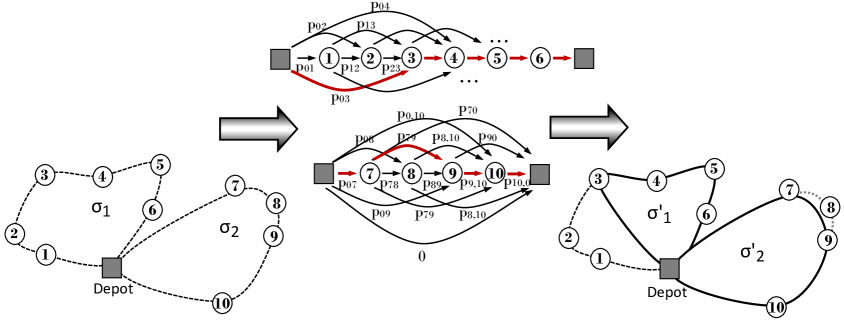
Figure 1: From an exhaustive solution to a VRPP solution

Each resource constrained shortest path problem is solved by dynamic programming. A label $s=(s^{\textsc{r}},s^{\textsc{p}})$ is defined as a couple (resource,profit). To each node $\sigma(i)$, for $i\in\{1,\dots,|\sigma|\}$ a set of labels ${\cal S}_{i}$ is associated, starting with ${\cal S}_{1}=\{(0,0)\}$ for the node representing the depot. Then, for any $i$, a set of labels ${\cal S}^{\prime}_{i+1}$ is constructed by considering iteratively any edge $(j,i+1)\in{\cal A}$ and extending all labels of $j$ as in Equation (9).

$${\cal S}^{\prime}_{i+1}=\bigcup_{j|(j,i+1)\in{\cal A}}\bigcup_{s_{j}\in{\cal S}_{j}}(s_{j}^{\textsc{r}}+r_{\sigma(j)\sigma(i+1)},s_{j}^{\textsc{p}}+p_{\sigma(j)\sigma(i+1)})$$ (9)

Any infeasible label $s\in{\cal S}^{\prime}_{i+1}$, such that $s^{\textsc{r}}+r_{\sigma(i+1)\sigma(0)}>R$ is pruned from ${\cal S}^{\prime}_{i+1}$. Indeed, resource consumptions on edges satisfy the triangle inequality, and thus the resource consumption for returning to $v_{0}$ after $\sigma(i+1)$ on any path is greater or equal than $r_{\sigma(i+1)\sigma(0)}$. All dominated labels of ${\cal S}^{\prime}_{i+1}$, i.e. labels $(s^{\textsc{r}},s^{\textsc{p}})\in{\cal S}^{\prime}_{i+1}$ such that there exists $(\bar{s}^{\textsc{r}},\bar{s}^{\textsc{p}})\in{\cal S}^{\prime}_{i+1}$ with $s^{\textsc{r}}\geq\bar{s}^{\textsc{r}}$ and $s^{\textsc{p}}<\bar{s}^{\textsc{p}}$ are also removed to yield ${\cal S}_{i+1}$.

The resulting Select algorithm is pseudo polynomial, with a complexity of $O(n^{2}B)$, where $B$ is an upper bound on the number of labels per node.

4.2 Neighborhood search on the exhaustive solution

We now consider a combined local search procedure which applies classic VRP moves on the exhaustive solution representation. Evaluating the profitability of any move requires to use the Select algorithm on the newly created routes to find the optimal selection of customers. As such, insertions and removals of customers are implicitly managed within the selection process, instead of being explicitly considered by the local search.

In the proposed heuristics, we consider the standard VRP moves 2-opt, 2-opt*, Relocate, Swap and Cross of a maximum of two customers (Vidal et al. 2013). These moves are tested between pairs of nodes $(v_{i},v_{j})$ such that $v_{j}$ is among the $\Gamma$ closest nodes of $v_{i}$ (similarly to Johnson and McGeoch 1997 and Toth and Vigo 2003). Moves are enumerated in a random order, any improvement being directly applied. The method stops whenever all moves have been tried without success.

4.3 Illustrative example

i	$r_{0,i}$	$r_{i-1,i}$	$p_{ij}\ \forall j$
1	15	–	10
2	25	30	15
3	15	20	15
4	15	20	10
5	20	25	12
6	15	10	15
7	20	15	15
8	25	15	12
9	25	20	15
10	15	35	15
$R=100$
$r_{7,9}=25$, $r_{10,0}=15$
all other consumptions = $+\infty$
$\sigma$	$R(\sigma)$		$P(\sigma)$
(3,4,5,6)	85		52
(7,9,10)	95		45
(1,2,3,4)	100		50
(6,7,8,9)	90		57

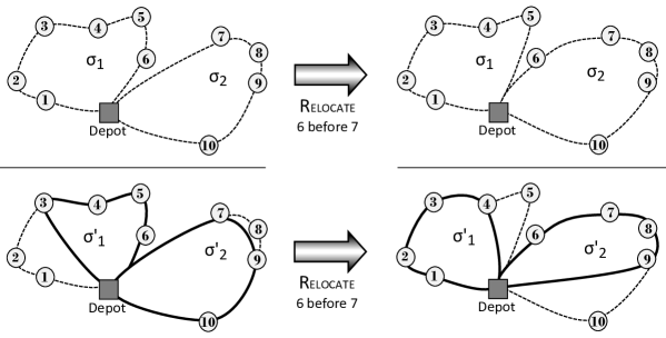
Figure 2: Relocate move on the exhaustive solution representation, and impact on the associated VRPP solution

Figure 2 illustrates a simple Relocate move of customer $v_{6}$ before $v_{7}$ on the exhaustive solution (top of the figure), and its impact on the associated VRPP solution (bottom of the figure). The initial VRPP solution, on the left, was a local-optimum of all classic neighborhoods. The Relocate move has a dramatic impact on the associated VRPP solution, since the Select algorithm operates different choices as a consequence, here a compound Removal of $v_{5}$ and $v_{10}$ and Insert of $v_{1}$ and $v_{2}$ before $v_{3}$. As a result, a feasible solution with higher profit is attained.

4.4 Connections with other large neighborhoods

The proposed methodology is distinct from the Split algorithm (Beasley 1983, Prins 2004), which aims to find the best segmentation of a permutation of customers into separate routes by inserting visits to the depot. In particular, we applied these neighborhoods within a Unified Hybrid Genetic Search with giant-tour “exhaustive” solution representation (Section 5.1). In this context, the Split algorithm can be implemented as a by-product of route evaluation procedures (Vidal et al. 2014a), and it assumes the twofold task of inserting depot visits and selecting customers.

These concepts are also clearly distinct from efficient ejection chains (Glover 1996) and cyclic improvement procedures based on the search for a positive-cost cycle in an auxiliary improvement graph. In our case, multiple compound Insert or Remove can implicitly arise from a move. The two methodologies could even be combined together by considering ejection chains on the exhaustive representation, and thus, searching a positive cycle in an auxiliary graph in which each arc cost has been obtained by means of the Select algorithm. This is left as a perspective of research.

4.5 Hierarchical objective

The total profit is usually not straightforward to improve with local and even large-neighborhood search, since it requires the ability to create space in order to save resources and deliver more profitable customers. An improvement of the objective is thus often the result of several combined moves. For the TOP in particular, the search space has a staircase aspect since multiple solutions have equal profit. This is usually not well-suited for an efficient search. To avoid this drawback and drive non-activated customers towards promising locations, the total distance of the current exhaustive solution is considered as a secondary objective (Equation 10) with very small weight $\omega\ll 1$.

$$Z^{\prime}=Z_{\textsc{2-vrpp}}(\sigma)+\omega\sum_{\sigma\in{\mathcal{R}}}\sum\limits_{i\in\{1,\dots,|\sigma|-1\}}d_{\sigma(i)\sigma(i+1)}$$ (10)

As a result, even if no improving move for the primary objective of the VRPP can be found from an incumbent solution, the neighborhood search will re-arrange the deliveries in better positions. This may open the way to new improvements of the main objective at a later stage, without requiring any solution deterioration.

4.6 Speed-up techniques

Solving from scratch each such resource constrained shortest path leads to computationally expensive move evaluations in $O(n^{2}B)$. Such near-quadratic complexity may not be acceptable in recent neighborhood-based heuristic searches which rely on a considerable number of route evaluations.

4.6.1 Graph sparsification

To reduce this complexity, we propose to prune several arcs in the shortest-path graph, and rely on pre-processing and bi-directional dynamic programming. For a given sparsification parameter $H\in\mathbb{N^{+}}$, only arcs $(i,j)$, with $(i<j)$ satisfying Equation (11) are kept.

$$j<i+H\text{ or }i=0\text{ or }j=|\sigma|$$ (11)

$H$ imposes an upper bound on the number of consecutive non-activated deliveries which can arise in a VRPP solution. The number of non-activated deliveries located just after or before a depot still remains unlimited, thus guaranteeing the existence of a feasible solution. This sparsification parameter is illustrated on Figure 3.

Figure 3: Shortest path graph after sparsification (H=3)

Proposition 3.

After sparsification, the number of arcs $|{\cal A}^{\prime}|$ in the new auxiliary graph ${\cal H}^{\prime}=({\cal V},{\cal A}^{\prime})$ becomes $O(n+n+Hn)=O(nH)$. The first two terms are the arcs originating and ending at the depot, and the term $Hn$ relates to the limited number of intermediate arcs. The complexity of Select becomes $O(nHB)$.

4.6.2 Labels pre-processing and route evaluations by concatenation

Solutions resulting from classic VRP moves on an incumbent exhaustive solution can all be assimilated to recombinations of a bounded number of subsequences of consecutive visits from this solution. This property is thoroughly discussed in Vidal et al. (2014b, a). As a consequence, we propose advanced move evaluation methods which pre-process additional information on subsequences of consecutive customers from the incumbent solution to reduce the complexity of move evaluations.

There are $O(n^{2})$ subsequences of consecutive customers in the incumbent solution. Pre-processing is done on these sequences, and the values are updated through the search whenever some routes of the incumbent solution are modified. As will be shown in the following, the effort related to information preprocessing is compensated by the reduction in computational effort related to move evaluations. In this section, we explain how this concept can be exploited to reduce even further the complexity of the Select algorithm for VRPPs.

For ease of presentation, we will call “starting node of $\sigma$” any node among the $H$ first nodes of $\sigma$, and “finish node of $\sigma$” any node among the H last nodes of $\sigma$. As in previous papers, we explain 1) the nature of the information, 2) how to do the preprocessing and 3) how to create an advanced Select algorithm which evaluates moves as a concatenation of known subsequences, using the information of each subsequence.

Information collected and preprocessing. For any subsequence $\sigma$ of consecutive nodes from the incumbent solution, the following information is pre-processed:

• Set of non-dominated labels $S_{ij}(\sigma)$ obtained from a resource constrained shortest path from a starting node $i$ to a finish node $j$ of $\sigma$. This information is computed for $i\in\{1,\dots,\min(H,|\sigma|)\}$ and $j\in\{\max(|\sigma|-H+1,1),\dots,|\sigma|\}$.

• Set of non-dominated labels $S^{\textsc{end}}_{i}(\sigma)$ obtained from a resource constrained shortest path in $\sigma$ from a starting node to the ending depot, for $i\in\{1,\dots,\min(H,|\sigma|)\}$.

• Set of non-dominated labels $S^{\textsc{beg}}_{j}(\sigma)$ obtained from a resource constrained shortest path in $\sigma$ from the starting depot to a finish node $j$, for $j\in\{\max(|\sigma|-H+1,1),\dots,|\sigma|\}$.

• Maximum profit $P(\sigma)$ of a feasible path within $\sigma$, which starts from the depot, visits a subset of customers in $\sigma$, and comes back to the depot.

Preprocessing these values for all sequences $\sigma$ requires $O(n^{2}HB)$ elementary operations. Indeed, the non-dominated labels associated to the all-pairs resource constrained shortest path in graph ${\cal H}^{\prime}$, between any node $i$ and $j$ (including the depot nodes), provide the required information. These labels are computed by forward labeling in $O(n\cdot nHB)$.

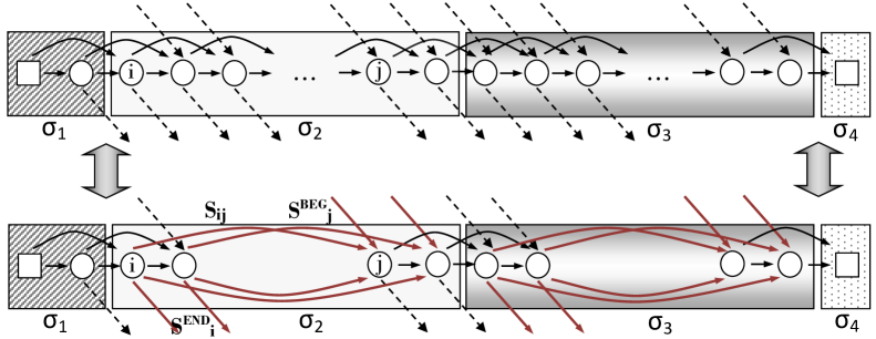
Figure 4: Using pre-processed information to reduce the graph (H=2)

Now, the contribution of this preprocessed information is illustrated in Figure 4. The top of the figure illustrates a shortest path problem in graph ${\cal H}^{\prime}$, for a new route involving four known subsequences. The edges in dotted lines are the ones originating or ending at the depot nodes. Here $H=2$, and thus it is possible to skip only one node at a time.

Remark that only arcs originating from the depot or finish nodes are connected to starting nodes in the next subsequence. Thus, any optimal path in the graph ${\cal H}^{\prime}$ visiting customers from more than two distinct sequences $\{\sigma_{x},\dots,\sigma_{y}\}$ must visit at least one starting node or finish node in each of these subsequences $\sigma_{k}\in\{\sigma_{x},\dots,\sigma_{y}\}$. As such, the partial path within a subsequence $\sigma_{k}$, either linking a starting node $i$ to a finish node $j$, or a starting node $i$ to the depot, or the depot to a finish node $j$, is represented by a label in $S_{ij}(\sigma_{k})$, $S^{\textsc{end}}_{i}(\sigma_{k})$ or $S^{\textsc{beg}}_{j}(\sigma_{k})$, respectively. These pre-processed labels can be introduced as new arcs in the graph, and they replace previous intermediate arcs and nodes within the sequence. This leads to a new shortest path problem in a graph ${\cal G}^{\prime\prime}$ illustrated in the bottom of the figure.

The new reduced graph ${\cal G}^{\prime\prime}=({\cal V}^{\prime\prime},{\cal A}^{\prime\prime})$ is such that $|{\cal A}^{\prime\prime}|=O(MH^{2})$ arcs and $|{\cal V}^{\prime\prime}|=O(MH)$ nodes. $M$ is a bounded value which stands for the number of subsequences. Classic intra-route moves for the VRP are such that $M\leq 3$, and all inter-route moves are such that $M\leq 5$ (Vidal et al. 2014b, a). The quantity of arcs $O(H^{2})$ does not depend anymore on the number of customers $n$. Still, the newly-created arcs, for any sequence $\sigma$, are not associated with a single profit and resource consumption, but rather to a set of non-dominated (resource, profit) couples $(s^{\textsc{r}},s^{\textsc{p}})\in S_{ij}(\sigma)$, such that $|S_{ij}(\sigma)|=O(B)$.

Proposition 4 (Concatenation – general).

The optimal profit $P(\sigma_{1}\oplus\dots\oplus\sigma_{M})$ of Select, for a route made of $M$ concatenated sequences $\sigma_{1}\oplus\dots\oplus\sigma_{M}$, is the maximum of the profit $\bar{P}(\sigma_{1}\oplus\dots\oplus\sigma_{M})$ of the resource constrained shortest path in ${\cal G}^{\prime\prime}$, and the maximum profit $P(\sigma_{i})$ of a feasible path within $\sigma_{i}$ exclusively, for $i\in\{1,\dots,M\}$:

$$P(\sigma_{1}\oplus\dots\oplus\sigma_{M})=\max\{\bar{P}(\sigma_{1}\oplus\dots\oplus\sigma_{M}),\max\limits_{i\in\{1,\dots,M\}}P(\sigma_{i})\}$$ (12)

$\bar{P}(\sigma_{1}\oplus\dots\oplus\sigma_{M})$ can be evaluated in $\Phi_{\textsc{C-M}}=O(MH^{2}B^{2})$.

Indeed, solving the shortest path on the reduced graph enables to find the best solution containing at least one starting or finish node. A better solution can exist, for each sequence $\sigma_{i}$, by visiting exclusively some inside nodes which have been eliminated in the reduced graph. The cost of these specific solutions is included in the preprocessed value $P(\sigma_{i})$. Now, the reduced graph ${\cal G}^{\prime\prime}$ has $O(MH^{2})$ arcs, and each arc is associated with up to $B$ non-dominated (resource, profit) couples. Solving the resource constrained shortest path on this graph to find $\bar{P}(\sigma_{1}\oplus\dots\oplus\sigma_{M})$ is equivalent to solving a resource constrained shortest path on a multi-graph, where arcs are duplicated $B$ times to take into account the different (resource,profit) combinations. This can be done as previously by means of a forward labeling method in $O(MH^{2}B^{2})$.

This algorithm derived from Proposition 4 is general in the sense that it can be used to evaluate a route made of any number of concatenated subsequences. Yet, it is used in our method only to evaluate moves which involve more than three subsequences, such as intra-route 2-opt, Swap and Relocate moves between two positions in the same route. The other – more numerous – inter-route Swap, Relocate, Cross and 2-opt* moves involve less than three subsequences (Vidal et al. 2013) as illustrated in Figure 5. Proposition 5 provides a way to evaluate these moves even more efficiently by means of bi-directional dynamic programming.

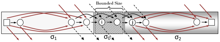
Figure 5: Route resulting from a concatenation of three subsequences

Proposition 5 (Concatenation – 3 subsequences).

The optimal cost $P(\sigma_{1}\oplus\sigma_{0}\oplus\sigma_{2})$ of Select, for a route made of three concatenated subsequences $\sigma_{1}\oplus\sigma_{0}\oplus\sigma_{2}$ such that $\sigma_{0}$ contains a bounded number of customers can be evaluated in $\Phi_{\textsc{C-3}}=O(H^{2}B).$ The same complexity is achieved for a concatenation of two sequences $\sigma_{1}$ and $\sigma_{2}$.

Indeed, the maximum of $\{P(\sigma_{1}),P(\sigma_{2})\}$ gives in $O(1)$ the best cost of a path that does not visit any starting or finish node in $\sigma_{1}$ or $\sigma_{2}$. Then, the best cost of a path visiting at least one starting or finish node can be evaluated as follows.

1. We recall that the set of non-dominated labels of a resource constrained shortest path going from the starting depot to a finish node $k$ of the first sequence $\sigma_{1}$ is given by $S^{\textsc{beg}}_{k}(\sigma_{1})$.

2. The algorithm propagates these labels iteratively to the next $|\sigma_{0}|$ nodes, obtaining the set of labels $\bar{S}_{i}(\sigma_{1,0})$ associated with the shortest path between the depot and the finish nodes of $\sigma_{1,0}=\sigma_{1}\oplus\sigma_{0}$, for $i\in\mathcal{I}=\{\max(|\sigma_{1}|+|\sigma_{0}|-H+1,1),\dots,|\sigma_{1}|+|\sigma_{0}|\}$. All arcs in $|\sigma_{0}|$ are simple arcs, such that each propagation is done in $O(HB)$. The propagation to the finish depot for each $i$ is also evaluated, leading in addition to the optimal cost $\bar{P}(\sigma_{1,0})$ of a path servicing at least one node in both $\sigma_{1}$ and $\sigma_{0}$ and returning to the end depot without visiting $\sigma_{2}$.

3. Finally, the best cost $\bar{P}(\sigma_{1,0}\oplus\sigma_{2})$ of a path servicing nodes in both $\sigma_{1,0}$ and $\sigma_{2}$ is equivalent to finding, for each possible arc $(i,j)\in{\cal A}^{\prime\prime}$ between $\sigma_{1,0}$ and $\sigma_{2}$, the best pair of labels $(s_{k}^{\textsc{r}},s_{k}^{\textsc{p}})\in\bar{S}_{i}(\sigma_{1,0})$ and $(s_{l}^{\textsc{r}},s_{l}^{\textsc{p}})\in S^{\textsc{end}}_{j}(\sigma_{2})$ which maximizes the total profit while respecting resource constraints as expressed in Equation (13).

   $$\bar{P}(\sigma_{1,0}\oplus\sigma_{2})=\max_{i\in\mathcal{I}}\max_{j\in\{1,\dots,\min(H,|\sigma_{2}|)\}}\left\{\begin{aligned} \max_{k,l}\ &\ s_{k}^{\textsc{p}}+p_{\sigma_{1,0}(i)\sigma_{2}(j)}+s_{l}^{\textsc{p}}\\ \text{s.t.}\ &\ s_{k}^{\textsc{r}}+r_{\sigma_{1,0}(i)\sigma_{2}(j)}+s_{l}^{\textsc{r}}\leq R\\ &(s_{k}^{\textsc{r}},s_{k}^{\textsc{p}})\in\bar{S}_{i}(\sigma_{1,0})\\ &(s_{l}^{\textsc{r}},s_{l}^{\textsc{p}})\in S^{\textsc{end}}_{j}(\sigma_{2})\end{aligned}\right\}$$ (13)

   For any $(i,j)$, the maximum cost of Equation (13) can be computed in $O(B)$ by sweeping the labels of $\bar{S}_{i}(\sigma_{1,0})$ by increasing resource consumption and, in the meantime, the labels of $S^{\textsc{end}}_{j}(\sigma_{2})$ by decreasing resource consumption.

   The computational complexity of the method is $O(|\sigma_{0}|HB)=O(HB)$ for Phase 2 and $O(H^{2}B)$ for Phase 3, leading to an overall complexity of $O(H^{2}B)$.

The final cost returned by the algorithm is

$$P(\sigma_{1}\oplus\sigma_{0}\oplus\sigma_{2})=\max\{\bar{P}(\sigma_{1,0}\oplus\sigma_{2}),\bar{P}(\sigma_{1,0}),P(\sigma_{1}),P(\sigma_{2})\}.$$ (14)

For the case involving only two sequences $\sigma_{1}$ and $\sigma_{2}$, the same algorithm without Phase 2 yields the same complexity.

Classic inter-route VRP neighborhoods contain $\Theta(n^{2})$ moves, for a total evaluation complexity of $\Theta(n^{2}H^{2}B)$ (c.f. Proposition 5). The complexity of the preprocessing phase is $O(n^{2}HB)$. Hence, move evaluation is dominating in terms of CPU time. This statement is also supported by our empirical analyses, which show that the additional preprocessing effort did not have a significant impact on CPU time.

Finally, intra-route moves are less numerous, in practice there are an average of $\Theta(\frac{n^{2}}{m})$ such moves to consider where $m$ is number of routes. The neighborhood evaluation complexity (c.f. Proposition 4) becomes $\Theta(\frac{n^{2}}{m}H^{2}B^{2})=\Theta(\frac{B}{m}n^{2}H^{2}B)$. The ratio $\frac{B}{m}$ is usually small and the observed effort spent on intra- and inter-route neighborhoods is of similar magnitude in our experiments.

5 Experimental Analyses

The contribution of this new large neighborhood is assessed by extensive computational experiments with three families of heuristics. The impact of key parameters is investigated on the TOP, and the performance of each method is evaluated on the TOP, as well as on the CPTP and VRPPFCC relatively to the current state-of-the-art solution methods.

5.1 Heuristics and metaheuristic frameworks

We selected three particular methods for our experiments: a multi-start local-improvement procedure (MS-LS), which represents one of the most simple scheme in heuristic search but is still at the core of most metaheuristics; a classic neighborhood-centered method such as the ILS of Prins (2009), and finally a more advanced population-based method with diversity management such as UHGS (Vidal et al. 2014a). This way, the contribution of the proposed neighborhoods can be investigated on three notable VRP heuristic frameworks.

• MS-LS is a straightforward application of the proposed neighborhood search, based on the classic neighborhoods 2-opt, 2-opt*, Relocate, Swap and Cross exchanges of up to two customers. As described previously, moves are applied between close customers on the exhaustive solution representation. A random order is used for move evaluation, any improving move being directly applied until no improvement can be found in the whole neighborhood. At the end, the resulting solution is a local optimum of the proposed neighborhood. The local-improvement procedure is repeated $\mu$ times from randomly generated initial solutions. The best local optimum constitutes the MS-LS solution.

• MS-ILS is a direct adaptation of the method of Prins (2009). Starting from a random initial solution, $n_{C}$ child solutions are iteratively generated by applying a shaking operator and the same local search as MS-LS. The best child solution is taken as new incumbent solution for the next iteration. The method is started $n_{P}$ times. Each run is completed once $n_{I}$ consecutive iterations have been performed without improvement of the best solution, or when an overall maximum time $T_{max}$ is attained. The overall best solution is finally returned.

• Finally, our implementation of UHGS derives directly from the general framework of Vidal et al. (2014a). The 2-VRPP has been addressed only by adding a new route-evaluation operator, and all other procedures, selection, crossover, education, Split algorithm and population-diversity management procedures remain the same. As previously, the population is managed to contain between $\mu^{\textsc{MIN}}$ and $\mu^{\textsc{MIN}}\nobreak+\nobreak\mu^{\textsc{GEN}}$ solutions, and the method terminates whenever $It_{max}$ iterations – individual generations – without improvement have been performed or when a CPU time $T_{max}$ is attained. No infeasible solutions need to be used in this context since the evaluation procedure allows for any route size without infeasibility.

5.2 Benchmark Instances

The performance of these three heuristics built on our new compound neighborhoods is assessed by means of extensive experiments on classic benchmark instances for the considered problems. The classic TOP instances (Chao et al. 1996) are classified into seven sets which include respectively 32, 21, 33, 100, 66, 64 and 102 customers. Each instance set is declined into individual instances with between 2 to 4 vehicles and different duration limits. We consider Sets 4-7, since optimal solutions are systematically obtained on the smaller problems. Other particular instances for which all methods from the recent literature find the optimal solutions have been also excluded from the experiments, only keeping the 157 most difficult ones as in Souffriau et al. (2010).

The CPTP instance sets of Archetti et al. (2009) have been derived from the classic VRP instances of Christofides et al. (1979) using different values of capacity $Q$ and fleet size $m$. We refer to each instance as “pXX-$m$-$Q$”, where XX is the index of the associated VRP instance. Finally, we rely for the VRPPFCC on the two sets of instances from Bolduc et al. (2008): Set “CE” is derived from the instances of Christofides et al. (1979) and includes up to 199 customers, while Set “G” includes larger instances with up to 483 customers, derived from Golden et al. (1998). Our three methods are compared to the best current metaheuristics in the literature, listed in Table 1.

Table 1: Methods, references and acronyms

Problem	Acronym	Method	Authors
TOP	TMH	Tabu Search	Tang and Miller-Hooks (2005)
	GTP	Tabu Search with Penalization Strategy	Archetti et al. (2007)
	GTF	Tabu Search with Feasible Strategy	Archetti et al. (2007)
	FVF	Fast Variable Neighborhood Search	Archetti et al. (2007)
	SVF	Slow Variable Neighborhood Search	Archetti et al. (2007)
	GLS	Guided Local Search	Vansteenwegen and Souffriau (2009)
	ASe	Ant Colony Optimization – Sequential	Ke et al. (2008)
	ADC	Ant Colony Optimization – Deterministic Concurrent	Ke et al. (2008)
	ARC	Ant Colony Optimization – Random Concurrent	Ke et al. (2008)
	ASi	And Colony Optimization – Simultaneous	Ke et al. (2008)
	SVNS	Skewed Variable Neighborhood Search	Vansteenwegen et al. (2009a)
	FPR	Fast Path Relinking	Souffriau et al. (2010)
	SPR	Slow Path Relinking	Souffriau et al. (2010)
	SA	Simulated Annealing	Lin (2013)
	MSA	Multi-Start Simulated Annealing	Lin (2013)
CPTP	GTP	Tabu Search with Admissible Strategy	Archetti et al. (2009)
	GTF	Tabu Search with Feasible Strategy	Archetti et al. (2009)
	VNS	Variable Neighborhood Search	Archetti et al. (2009)
VRPPFCC	SRI	Selection, Routing and Improvement	Bolduc et al. (2008)
	RIP	Randomized Construction-Improvement-Perturbation	Bolduc et al. (2008)
	TS	Tabu Search	Côté and Potvin (2009)
	TS2	Tabu Search with Ejection Chains	Potvin and Naud (2011)
	TS+	Tabu Search with Ejection Chains	Potvin and Naud (2011)
	AVNS	Adaptive Variable Neighborhood Search	Stenger et al. (2012)

5.3 Parameter setting and sensitivity analyses

General parameter setting. The proposed methodology relies on two parameters: the weight $\omega$ of the secondary objective and the sparsification coefficient $H$. The only purpose of $\omega$ is to establish a hierarchy between the real problem objective and the auxiliary route length objective (Section 4.5). From our experiments, setting $\omega=10^{-4}$ establishes the desired hierarchy without involving numerical precision issues. The impact of the sparsification coefficient $H$ is discussed later in this section.

For the other parameters, we aimed to implement the methods without significant changes from the original papers (Prins 2009, Vidal et al. 2014a). Still, to compare with other authors with similar computational effort, we had to scale the termination criteria and population size, leading to the setting $\mu=5$ for MS-LS, $(n_{\textsc{P}},n_{\textsc{I}},n_{\textsc{C}})=(3,10,3)$ for MS-ILS, and $(\mu^{\textsc{MIN}},\mu^{\textsc{GEN}},It_{max})=(5,10,500)$ for UHGS. The overall CPU time is also limited to $T_{max}=300s$.

Sensitivity analysis on the sparsification parameter. Parameter $H$ is an important element of the newly proposed neighborhoods. Larger values of this parameter lead to larger neighborhoods but higher CPU time. A good balance is thus desired. To calibrate $H$ and analyze its impact on the method, we ran several tests on the UHGS with values of $H\in\{1,2,3,5,7,10,\infty\}$. Each parameter configuration was tested on the 157 TOP benchmark instances and 10 runs have been conducted. The solution quality is measured for each instance as a percentage of deviation from the Best Known Solution (BKS) in the literature, $100(z_{\textsc{bks}}-z)/z_{\textsc{bks}}$, where $z$ is the profit obtained by the method and $z_{\textsc{bks}}$ is the profit of the BKS. The best known solutions, including those found in this paper, are included in Table 7.

The results of this calibration, averaged on all instances, are displayed in Table 2. We report for each configuration the average deviation to BKS on 10 runs, the deviation of the best solution of these runs, the number of BKS found out of 157, the average CPU time, the average CPU time to reach the best solution of the run, and the number of labels per customer node in the shortest path subproblems. Finally, the last line reports the p-values of a Wilcoxon signed-rank test for paired samples, between the average profit obtained with the reference parameter setting $H=3$ and any other setting $x$. The p-value illustrates how likely is the null hypothesis “that both methods for $H=3$ and $H=x$ perform equally”.

Table 2: Calibration of the sparsification parameter $H$

	H=1	H=2	H=3	H=4	H=5	H=7	H=10	H=$\infty$
Avg Gap	0.090%	0.022%	0.020%	0.035%	0.036%	0.055%	0.087%	0.177%
Best Gap	0.008%	0.002%	0.001%	0.002%	0.005%	0.005%	0.010%	0.016%
Nb BKS	144	155	155	153	152	152	148	143
Avg Time(s)	136.83	174.32	192.00	211.23	223.54	236.48	247.87	282.81
Avg T-Best(s)	84.89	92.54	91.09	103.10	111.19	118.82	130.40	156.86
Avg Labels	8.39	29.19	34.70	36.63	36.90	36.50	35.27	32.81
P-value	2.4E-12	0.23	–	1.5E-4	2.1E-5	5.5E-7	2.2E-8	3.0 E-11

From these tests, it appears that the configuration $H=3$ produces solutions of significantly better quality than any configuration with $H\in\{1,4,5,7,10,+\infty\}$. This configuration attains 155/157 best known solutions. It requires $40.3\%$ more CPU time than with $H=1$, but only $7.3\%$ more CPU time to reach the best solution. The average number of non-dominated labels kept per node is greater by a factor $4.4$ than the case with $H=1$. It should be noted that $H=1$ is not equivalent to “no selection”, since any arc from and to the depot is still considered, and thus the shortest path can select any subset of consecutive customers. Thus the number of labels for $H=1$ is greater than one. Using the selection abilities of the algorithm, and thus values of $H$ greater than one, contributes to find solutions of higher quality in similar CPU time.

Sensitivity analysis on the auxiliary objective.

We also tested the impact of the auxiliary objective by comparing a version in which this objective is not considered, i.e. $\omega=0$ to our base version. In these tests, and in the remainder of this paper, the value $H=3$ is used for the sparsification parameter. The results are presented in Table 3 in the same format as previously.

Table 3: Calibration of the auxiliary objective

	Auxiliary	Only Primary
	$\omega=10^{-4}$	$\omega=0$
Avg Gap	0.020%	0.102%
Best Gap	0.001%	0.006%
Nb BKS	155	150
Avg Time(s)	192.00	154.38
Avg T-Best(s)	91.09	56.43
Avg Labels	34.70	30.74
P-value	–	$5.1\cdot 10^{-13}$

Our results indicate a significant improvement, with a very small p-value of $5.1\cdot 10^{-13}$, of the solution quality related to the use of the auxiliary objective during optimization. The auxiliary objective leads to deeper local optimums, and thus potentially longer descents. This is illustrated by an increase of $24.4\%$ of the average CPU time, and $61.4\%$ of the average time to find the best solution. Yet, as a consequence the solution quality is also much higher. In particular, the average gap to BKS is reduced from $0.102\%$ to $0.020\%$ when the auxiliary objective is used. Even by using longer runs or multiple runs without this objective, it would take much longer CPU time to reach such solution quality.

5.4 Results on TOP

In this section, we compare the results generated by our methods to those generated by the previous state-of-the-art algorithms for the TOP, listed in Table 1. For this problem, several authors have reported results with very small CPU time, and thus to provide further elements of comparison we also created a fast version of UHGS, named UHGS-f, by reducing the termination criteria to $(It_{max},T_{max})=(250,60s)$.

Tables 7-9 (in Appendix) provide detailed results on the 157 selected instances, in comparison to the best previous methods, as well as the new BKS, merging previously-known solutions and a few improved ones found by the proposed methods. When a method finds the BKS, this solution is highlighted in boldface. When a new improved BKS is found, this solution is also underlined.

Table 4 provides a summary of these results. It displays for each method the average deviation to BKS on 10 runs, the average CPU time T(s) and average time T*(s) to reach the final solution of a run, the deviation to BKS of the best solution out of 10 runs, the associated total CPU time, and the processor used in the tests. A last line reports the p-value of a Wilcoxon test on paired samples between the best solutions of UHGS and other methods. Detailed CPU times, on each instance, are available from the authors. Most of the previous authors only report their best solution out of ten runs. Thus the CPU time of these solutions, as well as the CPU time of our best solution out of ten runs, is scaled by a factor of ten.

Table 4: Summary of results on the TOP

		FVF	SVF	ASe	FPR	SPR	MSA	UHGS	UHGS-f	MS-ILS	MS-LS
Avg	Gap	–	–	1.094%	–	–	–	0.020%	0.100%	0.115%	0.861%
	T(s)	18.9	458	25.2	5.00	21.2	–	192	69.0	156	9.29
	T*(s)	–	–	–	–	–	36.3	91.1	42.1	104	5.24
Best	Gap	0.189%	0.039%	0.088%	0.401%	0.052%	0.028%	0.001%	0.006%	0.003%	0.109%
	T(s)	56.7	1370	252	50.0	212	–	1920	690	1560	92.9
	Nb${}_{\textsc{BKS}}$	94	134	128	78	126	133	155	150	153	115
	CPU	P4 2.8G	P4 2.8G	PC 3G	Xe 2.5 G	Xe 2.5G	C2 2.5G	Xe 3.07G	Xe 3.07G	Xe 3.07G	Xe 3.07G
	P-val	5.2E-12	2.0E-05	3.9E-06	1.1E-14	1.2E-06	1.8E-05	***	4.3E-02	0.36	1.6E-08

The TOP results from methods in Table 1 are displayed in Figure 7 on a two-dimensional plot considering CPU time and Gap(%), using a logarithmic scale. The DEC AlphaServer 1200/533 and DEC Alpha XP 1000 CPUs of Tang and Miller-Hooks (2005) are approximately $5\times$ to $10\times$ slower than a Pentium IV 2.8 GHz according to Dongarra factors. The associated CPU time has thus been scaled accordingly. Due to a lack of accurate data, the speed of the other processors can not be scaled in a reliable manner. These processors are of similar generation and should not differ by a speed factor of more than $2\times$. Figure 7 thus displays a reasonable approximation of computation effort. Finally, it should be noted that Lin (2013) reports the time to reach the best solution, which is smaller than the total computational time, and thus receives a significant advantage.

Overall, the proposed UHGS with large neighborhood search produces solutions of high quality, reaching a small gap of $0.001\%$. This is a significant improvement over previous methods, as confirmed by the paired-samples Wilcoxon tests, with p-values smaller than $2\cdot 10^{-5}$. MS-ILS and MS-LS also obtain good solutions: the multi-start local improvement algorithm produces results of a quality comparable to current metaheuristics while being conceptually much simpler. A total of 155/157 best known solutions have been found by UHGS, as well as three new BKS (1267 for p4.2.q, 1292 for p4.2.r, and 1120 for p7.3.t).

The new methods with large neighborhoods, on the other hand, require a higher CPU time. For example, UHGS uses an average search time of 192 seconds, 91.1 seconds to find the final solution of the run, compared to 36.0 seconds to find the final solution for the previous best method, MSA. The CPU time of UHGS-f – 42.1 seconds to find the solution – is much closer to MSA. This increased time is due to the new neighborhoods, which require additional evaluation effort. To speed up the search, promising research avenues can consider the hybridization of the combined local search with more classic approaches, by applying CLS only on selected elite solutions.

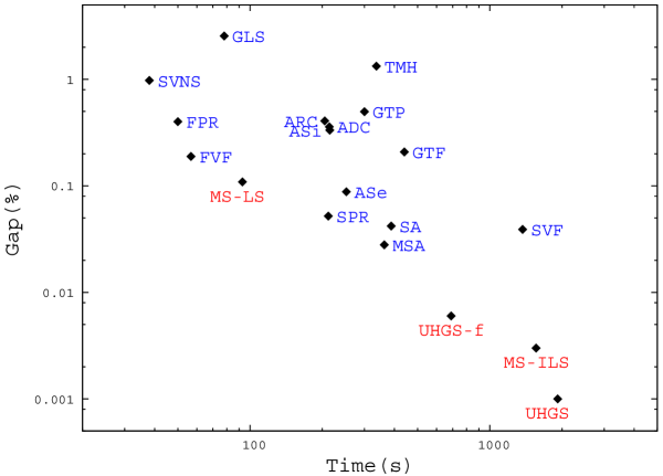
Figure 6: Trade-off between solution quality and CPU time – TOP benchmark instances

Figure 7 highlights a wide range of alternative trade-offs between computational time and solution quality. Nine methods are in the pareto front (SVNS, FPR, FVF, SPR, MSA along with the four proposed methods) and thus, depending on the application context and the desired solution quality, a wide panel of methods with different levels of sophistication is available.

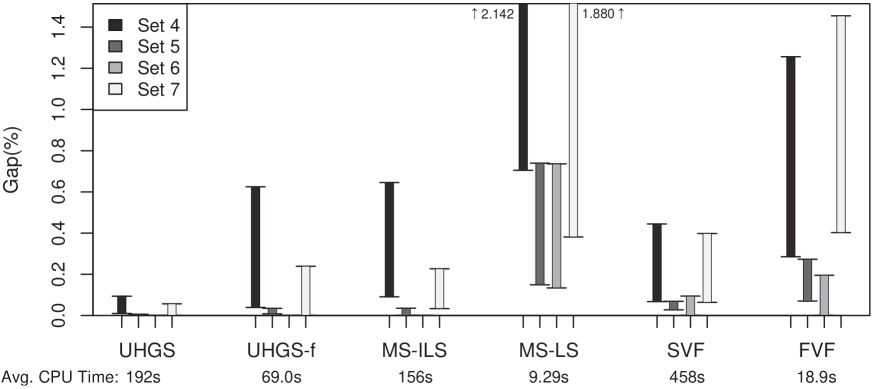
Figure 7: Range of solutions for each method and each set of instances. The top of each interval represents the worst solution of three random runs, while the bottom represents the best solution out of three runs.

Finally, in a similar fashion as Archetti et al. (2007), Figure 7 displays an analysis of the worst and best solutions on three random runs. The data associated with this figure is provided in Table 10, in appendix. The figure analyzes the robustness of methods, i.e., by how much solution quality may vary from one run to another. It appears that UHGS with large neighborhoods produces stable results (in 192 seconds per run) of overall higher quality than SVF (in 458 seconds per run) and other methods. A trade-off between computational effort and robustness is clearly observable. FVF appears is more stable than MS-LS, and requires less CPU time. Thus, the use of metaheuristic strategies still remains a good asset to achieve more stable results.

5.5 Results on other problems

Further experiments have been conducted on the VRPPFCC and CPTP. A summary of the results is displayed in Tables 5-6 and Figure 8, using the same conventions as previously. Average results, representative of a single run, are located with a triangle on this figure, while best solutions on ten runs are located with a diamond. The p-values in tables refer to statistical tests on the significance of the performance difference between the best solutions of UHGS and those of other methods. Detailed results per instance are provided in appendix.

Table 5: Summary of results on the VRPPFCC

		RIP	TS	TS 2	TS+	AVNS	UHGS	MS-ILS	MS-LS
Avg	Gap CE	1.104%	0.408%	–	–	–	0.153%	0.331%	2.862%
	Gap	1.575%	0.698%	–	–	–	0.272%	0.682%	3.155%
	T(min)	17.45	5.77	14.21	34.86	11.94	26.39	16.61	1.89
Best	Gap CE	–	0.165%	0.432%	0.319%	0.202%	0.016%	0.070%	1.505%
	Gap	–	0.405%	0.934%	0.228%	0.422%	0.038%	0.270%	2.100%
	T(min)	–	57.74	142.11	348.59	119.44	263.95	166.15	18.88
	Nb${}_{\textsc{BKS}}$	0	–	–	–	3	25	11	1
	CPU	Xe 3.6G	Opt 2.2G	Opt 2.2G	Opt 2.2G	I5 2.67G	Xe 3.07G	Xe 3.07G	Xe 3.07G
	P-val	6.5E-07	4.3E-02	2.1E-03	4.2E-03	1.2E-05	–	4.9E-04	5.4E-07

¹ Potvin and Naud (2011) performed experiments with the same TS algorithm of Côté and Potvin (2009), yet the reported solution quality (TS 2) is lower than in the original paper. We display both set of results, but note that there may be a high variance of solution quality.

² Côté (2013) reported to us that on Set “G”, truncated distances have been erroneously used for CP09 and PN11. The related solutions and gaps, reported in italics, can thus be considered only as lower bounds.

Table 6: Summary of results on the CPTP

		VNS	GTF	GTP	UHGS	MS-ILS	MS-LS
Avg	Gap	0.371%	0.952%	0.929%	0.030%	0.173%	0.557%
	T(min)	10.30	2.82	8.54	3.53	3.43	0.18
Best	Gap	–	–	–	0.001%	0.015%	0.154%
	T(min)	–	–	–	35.28	34.31	1.85
	Nb${}_{\textsc{BKS}}$	99	71	67	130	125	29
	CPU	PIV 2.8G	PIV 2.8G	PIV 2.8G	Xe 3.07G	Xe 3.07G	Xe 3.07G
	P-val	8.4E-06	1.4E-13	1.3E-13	–	4.3E-02	8.6E-02

For both problems, it is noteworthy that UHGS with the large neighborhood produces solution of better quality than the previous best methods. For the CPTP, a smaller CPU time is also achieved in most cases. For the VRPPFCC, a gap to the BKS of $0.038\%$ is obtained, compared to $0.228\%$ for TS+, which was, in addition, advantaged because of a distance rounding issue (c.f. note in Table 5). The average solutions on one run of UHGS, with a gap of $0.272\%$, are also of higher quality than the best solutions of AVNS on ten runs, with a gap of $0.422\%$, while requiring less overall CPU time. UHGS produces a large number of best known solutions (25/34), including 20 new ones. For the CPTP, UHGS reaches a total of 130/130 best known solutions, including 29 new ones, and all optimal solutions known from Archetti et al. (2009) and Archetti et al. (2013a) have been retrieved. MS-LS, MS-ILS and UHGS, lead to different CPU time and solution quality trade-offs, the fastest computation time being achieved with the simple MS-LS.

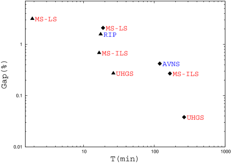
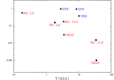
Figure 8: Trade-off between solution quality and CPU time – VRPPFCC (on the left) and CPTP (on the right). Comparison with state-of-the-art methods.

On Figure 8, the trade-off between solution quality and CPU time is visible for both problems. The proposed methods are dominating, since for any past method there exist at least one of our configurations which produces solutions of higher quality in less CPU time. We also note that, while the stand-alone MS-LS turned out to be very efficient on the TOP, its performance on the VRPPFCC tends to be lower. This can be related to the fact that the objective of VRPPFCC or CPTP is based on both customer selection and routing. For the TOP, the selection alone is considered in the objective, and slightly sub-optimal routing decisions may only weakly impact the sets of feasible selections considered by the method.

6 Conclusion

We have introduced a new large neighborhood for VRPs with profits. These neighborhoods are searched by means of efficient pruning and bi-directional dynamic programming techniques. They have been tested in a local-improvement method, an iterated local search and a hybrid genetic search, on the TOP, the CPTP and the VRPPFCC. These new neighborhoods contribute to find solutions of higher quality in comparison to the previous state-of-the-art methods. 52 new best known solutions have been found. It is remarkable that the simple local-improvement method with these neighborhoods reaches solutions of similar quality than most current complex metaheuristics for the TOP.

The proposed method is a very novel way of designing neighborhood search on VRP with profits. It should be more successful on settings for which the ratio of customers to be delivered is high, such as the VRPPFCC where a small proportion of deliveries are usually assigned to a third party provider. Problems with a large number of delivery options, e.g. thousands of locations, and scarce resources, e.g. trucks to service only a few customers, may still not be well suited for such methodology, since all deliveries are considered in the routing algorithm. To efficiently handle both cases, we suggest as a perspective of research to hybridize classic and new neighborhoods. The classic neighborhood can help filtering subsets of more promising deliveries, and generating elite initial solutions, which can then be improved by a few iterations of the large neighborhoods with subsets of potential customers. This would allow to harness the highest exploration capacities of our proposed neighborhood search while reducing even further the CPU time. Other perspective of research involve the extension of the proposed methodologies to other variants of VRPP, e.g., with time windows, variable profits, or arc routing, and even more general extensions of the concepts to other combinatorial optimization problems with decisions on task selections.

Table 7: Results for the TOP, instances of Chao et al. (1996)

Inst	FVF	ASe	FPR	SPR	MSA	UHGS		UHGS-f		MS-ILS		MS-LS		BKS
						Avg	Best	Avg	Best	Avg	Best	Avg	Best
p4.2.a	206	206	206	206	206	206	206	206	206	206	206	206	206	206
p4.2.b	341	341	341	341	341	341	341	341	341	341	341	340	341	341
p4.2.c	452	452	452	452	452	452	452	452	452	452	452	450.8	452	452
p4.2.d	531	531	531	531	531	531	531	531	531	531	531	526.1	531	531
p4.2.e	618	618	612	618	618	618	618	617	618	618	618	603.7	613	618
p4.2.f	684	687	687	687	687	685.2	687	683.9	687	683.4	687	675.9	687	687
p4.2.g	750	757	757	757	757	755.2	757	754.4	757	754.7	757	742.5	752	757
p4.2.h	827	827	835	835	835	835	835	829.6	835	824.7	835	813.4	825	835
p4.2.i	916	918	918	918	918	918	918	904.7	918	899.5	918	878.3	918	918
p4.2.j	962	965	962	965	962	964.4	965	952.1	964	964.7	965	928	964	965
p4.2.k	1019	1022	1013	1022	1022	1022	1022	1018.2	1022	1008.8	1022	991.5	1022	1022
p4.2.l	1073	1071	1064	1074	1073	1074	1074	1066	1074	1050.1	1074	1050.8	1073	1074
p4.2.m	1132	1130	1130	1132	1132	1130.6	1132	1114.7	1132	1121.9	1132	1105.3	1132	1132
p4.2.n	1159	1168	1161	1173	1174	1172.4	1174	1163.5	1174	1167.3	1174	1161.7	1172	1174
p4.2.o	1216	1215	1206	1218	1217	1215.7	1218	1206.2	1218	1207.7	1218	1194.3	1213	1218
p4.2.p	1239	1242	1240	1242	1241	1239.2	1242	1234.9	1241	1236.2	1242	1221.8	1239	1242
p4.2.q	1265	1263	1257	1263	1259	1263.8	1267	1261.1	1267	1259.5	1267	1255	1262	1267
p4.2.r	1283	1288	1278	1286	1290	1286.4	1292	1280.7	1285	1282.1	1287	1274.6	1285	1292
p4.2.s	1300	1304	1293	1296	1300	1301.1	1302	1297.3	1302	1298.2	1304	1293.2	1301	1304
p4.2.t	1306	1306	1299	1306	1306	1306	1306	1305.7	1306	1305.7	1306	1304.1	1306	1306
p4.3.c	193	193	193	193	193	193	193	193	193	193	193	193	193	193
p4.3.d	335	335	333	335	335	335	335	335	335	335	335	333.7	335	335
p4.3.e	468	468	468	468	468	468	468	468	468	468	468	465.6	468	468
p4.3.f	579	579	579	579	579	579	579	579	579	579	579	572.5	579	579
p4.3.g	653	653	653	653	653	653	653	652.9	653	653	653	652.4	653	653
p4.3.h	724	720	725	729	729	729	729	729	729	729	729	715.1	728	729
p4.3.i	806	796	797	809	809	809	809	809	809	809	809	800.3	809	809
p4.3.j	861	861	858	861	860	861	861	860.7	861	859.9	861	850.6	861	861
p4.3.k	919	918	918	918	919	919	919	918.7	919	918.3	919	906.8	919	919
p4.3.l	975	979	968	979	978	979	979	978.6	979	978.1	979	964.3	979	979
p4.3.m	1056	1053	1043	1063	1063	1063	1063	1059.8	1063	1058.3	1063	1026.5	1051	1063
p4.3.n	1111	1121	1108	1120	1121	1121	1121	1120.8	1121	1118.2	1121	1087.2	1121	1121
p4.3.o	1172	1170	1165	1170	1170	1170.9	1172	1163.1	1170	1168.2	1172	1136.2	1170	1172
p4.3.p	1208	1221	1209	1220	1222	1222	1222	1213.6	1222	1220.3	1222	1190.7	1208	1222
p4.3.q	1250	1252	1246	1253	1251	1252.8	1253	1249.3	1253	1250.4	1253	1230.2	1253	1253
p4.3.r	1272	1267	1257	1272	1265	1271.5	1273	1269.8	1272	1269.9	1272	1258.5	1271	1273
p4.3.s	1289	1293	1276	1287	1293	1294.4	1295	1292.6	1295	1292.6	1295	1280.3	1290	1295
p4.3.t	1298	1305	1294	1299	1299	1304.2	1305	1303.6	1305	1302.4	1304	1296.9	1301	1305
p4.4.e	183	183	183	183	183	183	183	183	183	183	183	183	183	183
p4.4.f	324	324	324	324	324	324	324	324	324	324	324	322.6	324	324
p4.4.g	461	461	461	461	461	461	461	461	461	461	461	459.7	461	461
p4.4.h	571	571	571	571	571	571	571	571	571	571	571	556.1	571	571
p4.4.i	657	657	653	657	657	657	657	657	657	657	657	651.5	657	657
p4.4.j	732	732	732	732	732	732	732	732	732	732	732	725.7	732	732
p4.4.k	821	821	820	821	821	821	821	820.9	821	820.8	821	814.8	821	821
p4.4.l	879	880	875	879	880	880	880	879.9	880	879.7	880	858.9	880	880
p4.4.m	916	918	914	919	919	919	919	917.7	919	916.3	919	911.3	919	919
p4.4.n	968	961	953	969	975	975.2	976	969.5	976	969.1	976	959.4	967	977
p4.4.o	1051	1036	1033	1057	1061	1061	1061	1061	1061	1061	1061	1024.2	1057	1061
p4.4.p	1120	1111	1098	1122	1124	1124	1124	1124	1124	1124	1124	1100.1	1124	1124
p4.4.q	1160	1145	1139	1160	1161	1161	1161	1161	1161	1159.8	1161	1152.9	1159	1161
p4.4.r	1207	1200	1196	1213	1216	1216	1216	1212.2	1216	1211.4	1216	1190	1207	1216
p4.4.s	1259	1249	1231	1250	1256	1260	1260	1257.2	1260	1259.1	1260	1238.8	1259	1260
p4.4.t	1282	1281	1256	1280	1285	1284.4	1285	1283.4	1285	1282.3	1285	1266.6	1280	1285
p5.2.h	410	410	410	410	410	410	410	410	410	410	410	409	410	410
p5.2.j	580	580	580	580	580	580	580	580	580	580	580	580	580	580
p5.2.k	670	670	670	670	670	670	670	670	670	670	670	668.5	670	670
p5.2.l	800	800	800	800	800	800	800	800	800	800	800	797	800	800
p5.2.m	860	860	860	860	860	860	860	860	860	860	860	858	860	860
p5.2.n	925	925	925	925	925	925	925	925	925	925	925	924	925	925
p5.2.o	1020	1020	1020	1020	1020	1020	1020	1020	1020	1020	1020	1014	1020	1020
p5.2.p	1150	1150	1150	1150	1150	1150	1150	1150	1150	1150	1150	1148	1150	1150
p5.2.q	1195	1195	1195	1195	1195	1195	1195	1194.5	1195	1195	1195	1192.5	1195	1195
p5.2.r	1260	1260	1260	1260	1260	1260	1260	1260	1260	1260	1260	1258	1260	1260
p5.2.s	1340	1340	1340	1340	1340	1340	1340	1340	1340	1340	1340	1332.5	1340	1340
p5.2.t	1400	1400	1400	1400	1400	1400	1400	1400	1400	1400	1400	1391	1400	1400
p5.2.u	1460	1460	1460	1460	1460	1460	1460	1460	1460	1460	1460	1454	1460	1460
p5.2.v	1500	1505	1505	1505	1505	1505	1505	1505	1505	1505	1505	1498.5	1505	1505
p5.2.w	1560	1560	1560	1560	1565	1565	1565	1563	1565	1562.5	1565	1553	1560	1565
p5.2.x	1590	1610	1610	1610	1610	1610	1610	1610	1610	1610	1610	1599.5	1610	1610
p5.2.y	1635	1645	1645	1645	1645	1645	1645	1645	1645	1645	1645	1632.5	1640	1645

Table 8: Results for the TOP, instances of Chao et al. (1996) (continued)

Inst	FVF	ASe	FPR	SPR	MSA	UHGS		UHGS-f		MS-ILS		MS-LS		BKS
						Avg	Best	Avg	Best	Avg	Best	Avg	Best
p5.2.z	1670	1680	1670	1680	1680	1680	1680	1680	1680	1680	1680	1668.5	1680	1680
p5.3.k	495	495	495	495	495	495	495	495	495	495	495	492	495	495
p5.3.l	595	595	595	595	595	595	595	595	595	595	595	591.5	595	595
p5.3.n	755	755	755	755	755	755	755	755	755	755	755	755	755	755
p5.3.o	870	870	870	870	870	870	870	870	870	870	870	870	870	870
p5.3.q	1070	1070	1070	1070	1070	1069.5	1070	1070	1070	1070	1070	1068	1070	1070
p5.3.r	1125	1125	1125	1125	1125	1125	1125	1125	1125	1125	1125	1121.5	1125	1125
p5.3.s	1190	1190	1185	1190	1190	1190	1190	1190	1190	1190	1190	1189.5	1190	1190
p5.3.t	1260	1260	1260	1260	1260	1260	1260	1260	1260	1260	1260	1257	1260	1260
p5.3.u	1345	1345	1335	1345	1345	1345	1345	1345	1345	1345	1345	1340	1345	1345
p5.3.v	1425	1425	1420	1425	1425	1425	1425	1425	1425	1424	1425	1419.5	1425	1425
p5.3.w	1485	1485	1465	1485	1485	1485	1485	1484.5	1485	1483.5	1485	1467.5	1480	1485
p5.3.x	1555	1540	1540	1550	1555	1554	1555	1553	1555	1552	1555	1534	1535	1555
p5.3.y	1595	1590	1590	1590	1590	1592.5	1595	1590.5	1595	1590.5	1595	1584	1590	1595
p5.3.z	1635	1635	1635	1635	1635	1635	1635	1635	1635	1635	1635	1634.5	1635	1635
p5.4.m	555	555	555	555	555	555	555	555	555	555	555	554	555	555
p5.4.o	690	690	690	690	690	690	690	690	690	690	690	683	690	690
p5.4.p	765	765	760	760	765	765	765	763	765	764.5	765	761	765	765
p5.4.q	860	860	860	860	860	860	860	860	860	860	860	844.5	860	860
p5.4.r	960	960	960	960	960	960	960	960	960	960	960	946.5	960	960
p5.4.s	1030	1030	1005	1025	1030	1030	1030	1030	1030	1030	1030	1025	1030	1030
p5.4.t	1160	1160	1160	1160	1160	1160	1160	1160	1160	1160	1160	1160	1160	1160
p5.4.u	1300	1300	1300	1300	1300	1300	1300	1300	1300	1300	1300	1300	1300	1300
p5.4.v	1320	1320	1320	1320	1320	1320	1320	1320	1320	1320	1320	1318	1320	1320
p5.4.w	1390	1390	1380	1390	1390	1390	1390	1390	1390	1389.5	1390	1382.5	1390	1390
p5.4.x	1450	1450	1430	1450	1450	1450	1450	1450	1450	1450	1450	1440	1450	1450
p5.4.y	1520	1520	1520	1520	1520	1520	1520	1520	1520	1520	1520	1514	1520	1520
p5.4.z	1620	1620	1620	1620	1620	1620	1620	1620	1620	1620	1620	1601	1620	1620
p6.2.d	192	192	192	192	192	192	192	192	192	192	192	190.2	192	192
p6.2.j	948	948	942	948	948	948	948	948	948	948	948	945.6	948	948
p6.2.l	1116	1116	1110	1116	1116	1116	1116	1116	1116	1116	1116	1109.4	1116	1116
p6.2.m	1188	1188	1188	1188	1188	1188	1188	1188	1188	1188	1188	1182	1188	1188
p6.2.n	1260	1260	1260	1260	1260	1260	1260	1260	1260	1260	1260	1246.8	1254	1260
p6.3.g	282	282	282	282	282	282	282	282	282	282	282	279.6	282	282
p6.3.h	444	444	444	444	444	444	444	444	444	444	444	444	444	444
p6.3.i	642	642	642	642	642	642	642	642	642	642	642	642	642	642
p6.3.k	894	894	894	894	894	894	894	894	894	894	894	892.8	894	894
p6.3.l	1002	1002	1002	1002	1002	1002	1002	1002	1002	1002	1002	1000.8	1002	1002
p6.3.m	1080	1080	1080	1080	1080	1080	1080	1080	1080	1080	1080	1080	1080	1080
p6.3.n	1170	1170	1164	1170	1170	1170	1170	1170	1170	1170	1170	1167.6	1170	1170
p6.4.j	366	366	366	366	366	366	366	366	366	366	366	364.8	366	366
p6.4.k	528	528	528	528	528	528	528	528	528	528	528	528	528	528
p6.4.l	696	696	696	696	696	696	696	696	696	696	696	694.8	696	696
p7.2.d	190	190	190	190	190	190	190	190	190	190	190	190	190	190
p7.2.e	289	290	290	290	290	290	290	290	290	290	290	288.4	290	290
p7.2.f	387	387	387	387	387	387	387	387	387	387	387	386.1	387	387
p7.2.g	459	459	459	459	459	459	459	459	459	459	459	458.1	459	459
p7.2.h	521	521	521	521	521	521	521	521	521	521	521	519.8	521	521
p7.2.i	575	580	578	580	579	580	580	579.6	580	579.7	580	577.2	580	580
p7.2.j	643	646	646	646	646	646	646	646	646	646	646	638.5	646	646
p7.2.k	704	705	702	705	705	705	705	704.3	705	703.9	705	701.4	705	705
p7.2.l	759	767	759	767	767	767	767	767	767	767	767	759.2	767	767
p7.2.m	824	827	816	827	827	827	827	827	827	824.7	827	817	827	827
p7.2.n	883	888	888	888	888	887.6	888	882.4	888	880.7	888	869.4	884	888
p7.2.o	945	945	932	945	945	945	945	944.6	945	944.1	945	929.3	945	945
p7.2.p	1002	1002	993	1002	1002	1002	1002	999	1002	998.5	1002	983.4	1002	1002
p7.2.q	1038	1043	1043	1044	1043	1044	1044	1042.6	1044	1043	1044	1034.7	1044	1044
p7.2.r	1094	1094	1076	1094	1093	1093.4	1094	1090.8	1094	1087.6	1094	1077.6	1085	1094
p7.2.s	1136	1136	1125	1136	1135	1133.5	1136	1133.5	1136	1128.8	1136	1120.4	1133	1136
p7.2.t	1168	1179	1168	1175	1172	1176	1179	1166.6	1179	1165.2	1179	1159.9	1170	1179
p7.3.h	425	425	425	425	425	425	425	425	425	425	425	422.8	425	425
p7.3.i	487	487	485	487	487	487	487	487	487	487	487	484	487	487
p7.3.j	562	564	560	564	564	564	564	564	564	564	564	553.4	564	564
p7.3.k	632	633	633	633	633	633	633	633	633	633	633	626.2	633	633
p7.3.l	681	684	684	684	684	684	684	684	684	683.8	684	679	684	684
p7.3.m	745	762	762	762	762	762	762	760.9	762	762	762	745.8	762	762
p7.3.n	814	820	813	820	820	820	820	820	820	820	820	807	820	820
p7.3.o	871	874	859	874	874	874	874	874	874	874	874	866.9	874	874
p7.3.p	926	929	925	927	927	928.6	929	928	929	927.8	929	917.1	925	929
p7.3.q	978	987	970	987	987	987	987	985.4	987	985.4	987	970.3	984	987

Table 9: Results for the TOP, instances of Chao et al. (1996) (finished)

Inst	FVF	ASe	FPR	SPR	MSA	UHGS		UHGS-f		MS-ILS		MS-LS		BKS
						Avg	Best	Avg	Best	Avg	Best	Avg	Best
p7.3.r	1024	1026	1017	1021	1026	1025.8	1026	1024.1	1026	1022.9	1026	1016.1	1024	1026
p7.3.s	1079	1081	1076	1081	1081	1080.1	1081	1079.6	1081	1079.6	1081	1060.7	1074	1081
p7.3.t	1112	1118	1111	1118	1119	1119.2	1120	1117.9	1120	1116.9	1120	1105.7	1113	1120
p7.4.g	217	217	217	217	217	217	217	217	217	217	217	215.3	217	217
p7.4.h	285	285	285	285	285	285	285	285	285	285	285	284.4	285	285
p7.4.i	366	366	366	366	366	366	366	366	366	366	366	364.2	366	366
p7.4.k	518	520	518	518	520	519.2	520	519.4	520	519.8	520	516.2	520	520
p7.4.l	588	590	581	590	590	590	590	590	590	590	590	579.9	590	590
p7.4.m	646	646	646	646	646	646	646	646	646	646	646	640.1	646	646
p7.4.n	715	730	723	730	730	730	730	730	730	729.6	730	715.7	726	730
p7.4.o	770	781	780	780	781	781	781	781	781	780.6	781	769.8	777	781
p7.4.p	846	846	842	846	846	846	846	846	846	843.4	846	831.4	846	846
p7.4.q	899	909	902	907	909	909	909	908.9	909	908.8	909	896.3	904	909
p7.4.r	970	970	961	970	970	970	970	970	970	970	970	957.8	970	970
p7.4.s	1021	1022	1022	1022	1022	1022	1022	1022	1022	1022	1022	1013.7	1022	1022
p7.4.t	1077	1077	1066	1077	1077	1077	1077	1077	1077	1077	1077	1064.9	1077	1077

Table 10: Best and Worst solutions on three runs, in Gap(%)

		UHGS	UHGS-f	MS-ILS	MS-LS	SVF	FVF
Set 4	Best	0.009	0.038	0.090	0.704	0.067	0.284
	Worst	0.095	0.626	0.646	2.412	0.445	1.257
Set 5	Best	0.000	0.007	0.000	0.148	0.027	0.069
	Worst	0.007	0.036	0.036	0.740	0.070	0.274
Set 6	Best	0.000	0.000	0.000	0.133	0.000	0.000
	Worst	0.000	0.000	0.000	0.737	0.095	0.196
Set 7	Best	0.000	0.000	0.033	0.380	0.063	0.401
	Worst	0.058	0.240	0.228	1.880	0.399	1.456

Table 11: Results for the VRPPFCC, instances of Bolduc et al. (2008)

Inst	n	RIP	TS	TS-PN	TS+	AVNS	UHGS		MS-ILS		MS-LS		BKS
		Single	Best	Best	Best	Best	Avg	Best	Avg	Best	Avg	Best
p01	50	1132.91	1119.47	1119.47	1119.47	1123.95	1119.66	1119.47	1119.66	1119.47	1128.28	1121.32	1119.47
p02	75	1835.76	1814.52	1814.52	1814.52	1814.52	1815.63	1814.52	1817.34	1814.52	1883.44	1840.71	1814.52
p03	100	1959.65	1924.99	1921.10	1930.66	1920.86	1922.88	1919.05	1929.60	1922.18	1958.80	1943.64	1919.05
p04	150	2545.72	2515.50	2525.17	2525.17	2512.05	2509.82	2505.39	2516.12	2505.39	2568.49	2548.29	2505.39
p05	199	3172.22	3097.99	3113.58	3117.10	3099.77	3095.58	3081.59	3102.95	3090.53	3201.29	3181.86	3081.59
p06	50	1208.33	1207.47	1207.47	1207.47	1207.81	1207.47	1207.47	1207.56	1207.47	1216.57	1207.47	1207.47
p07	75	2006.52	2006.52	2006.52	2006.52	2013.93	2012.33	2006.52	2022.93	2006.52	2079.67	2046.62	2004.53
p08	100	2082.75	2055.64	2060.17	2056.59	2052.05	2057.57	2052.05	2062.21	2054.64	2100.59	2088.10	2052.05
p09	150	2443.94	2429.19	2438.43	2435.97	2432.51	2428.19	2425.32	2433.28	2428.03	2505.24	2478.01	2422.74
p10	199	3464.90	3393.41	3406.82	3401.83	3391.35	3387.12	3381.67	3393.78	3382.23	3491.59	3462.56	3381.67
p11	120	2333.03	2330.94	2353.39	2332.36	2332.21	2331.13	2330.94	2336.06	2330.94	2408.13	2343.03	2330.94
p12	100	1953.55	1952.86	1952.86	1952.86	1953.55	1953.13	1952.86	1953.13	1952.86	1982.06	1970.05	1952.86
p13	120	2864.21	2859.12	2882.70	2860.89	2858.94	2859.07	2858.83	2859.01	2858.83	3025.26	2909.83	2858.83
p14	100	2224.63	2214.14	2216.97	2216.97	2215.38	2213.02	2213.02	2213.02	2213.02	2226.44	2215.38	2213.02
pr01	240	14388.58	14214.44	14218.83	14190.01	14157.08	14151.51	14131.18	14165.45	14151.74	14329.96	14272.27	14123.38
pr02	320	19505.00	19609.62	19729.96	19208.52	19204.36	19190.77	19166.58	19191.56	19142.75	19524.50	19417.12	19142.75
pr03	400	24978.17	25271.50	25653.58	24592.18	24602.61	24588.29	24409.02	24609.36	24493.16	25038.41	24916.33	24409.02
pr04	480	34957.98	35068.47	36022.73	34802.08	34415.82	34517.47	34362.80	34907.49	34708.93	35182.78	34883.27	34275.11
pr05	200	14683.03	14486.14	14673.56	14261.31	14272.32	14296.07	14223.63	14373.87	14255.09	14735.12	14492.24	14223.63
pr06	280	22260.19	21690.25	22278.99	21498.03	21440.79	21488.29	21396.60	21546.18	21382.16	22024.07	21741.15	21382.16
pr07	360	23963.36	24112.79	24191.41	23513.06	23375.60	23463.05	23373.38	23547.12	23407.50	23980.00	23751.10	23373.38
pr08	440	30496.18	30466.04	30627.91	30073.56	29797.62	29918.06	29823.18	30064.28	29953.21	30459.11	30271.82	29712.97
pr09	255	1341.17	1323.57	1328.14	1325.62	1335.45	1332.63	1328.65	1339.06	1332.09	1397.08	1370.26	1328.65
pr10	323	1612.09	1592.93	1590.83	1590.82	1604.50	1603.82	1597.61	1617.58	1595.45	1682.31	1664.96	1595.45
pr11	399	2198.45	2166.66	2172.28	2173.80	2189.02	2192.68	2182.01	2228.23	2196.75	2281.79	2248.04	2182.01
pr12	483	2521.79	2490.01	2492.75	2495.02	2520.29	2529.84	2522.64	2553.40	2540.92	2652.57	2624.19	2520.29
pr13	252	2286.91	2271.29	2278.99	2274.12	2291.83	2261.50	2258.02	2277.57	2274.19	2337.43	2319.74	2258.02
pr14	320	2750.75	2693.35	2705.00	2703.31	2708.22	2687.50	2683.73	2708.56	2701.78	2791.23	2764.11	2683.73
pr15	396	3216.99	3157.31	3158.92	3161.26	3194.82	3152.00	3145.11	3177.53	3170.50	3296.86	3272.34	3145.11
pr16	480	3693.62	3637.52	3639.11	3638.39	3671.34	3632.04	3620.71	3672.62	3641.69	3811.80	3794.17	3620.71
pr17	240	1701.58	1631.49	1636.11	1633.35	1682.49	1671.72	1666.31	1677.37	1669.59	1717.55	1708.26	1666.31
pr18	300	2765.92	2692.49	2705.90	2710.21	2741.80	2733.12	2730.55	2741.10	2734.81	2801.70	2793.63	2730.55
pr19	360	3576.92	3452.00	3497.54	3497.72	3507.94	3504.26	3497.20	3515.47	3508.53	3585.64	3570.94	3497.20
pr20	420	4378.13	4272.98	4311.17	4306.89	4332.44	4319.37	4312.45	4333.59	4316.28	4433.41	4405.90	4312.45

Côté (2013) reported to us that on the set “G”, truncated distances have been erroneously used for CP09 and PN11. The related solutions and gaps, reported in italics, can thus be considered only as lower bounds on the performance of these algorithms.

Table 12: Results for the CPTP, instances of Archetti et al. (2009)

Inst	n	VNS	GTF	GTP	UHGS		MS-ILS		MS-LS		BKS
		Single	Single	Single	Avg	Best	Avg	Best	Avg	Best
p03-15-200	100	663.98	657.31	656.32	664.92	664.92	663.83	664.92	657.84	663.78	664.92
p03-2-50	100	57.75	57.75	57.75	57.75	57.75	57.75	57.75	57.75	57.75	57.75
p03-2-75	100	106.15	106.15	106.15	106.15	106.15	106.15	106.15	105.98	106.15	106.15
p03-2-100	100	158.21	158.21	158.21	158.21	158.21	158.21	158.21	158.17	158.21	158.21
p03-2-200	100	330.14	319.28	319.28	330.14	330.14	330.14	330.14	327.34	330.14	330.14
p03-3-50	100	80.82	80.82	80.82	80.82	80.82	80.82	80.82	80.82	80.82	80.82
p03-3-75	100	147.55	147.55	145.87	147.55	147.55	147.55	147.55	147.38	147.55	147.55
p03-3-100	100	218.63	218.63	218.33	218.63	218.63	218.63	218.63	218.19	218.63	218.63
p03-3-200	100	447.15	444.82	433.38	447.15	447.15	447.1	447.15	442.95	445.51	447.15
p03-4-50	100	100.36	98.47	100.36	100.36	100.36	100.36	100.36	100.17	100.36	100.36
p03-4-75	100	185.27	185.27	185.27	185.27	185.27	185.27	185.27	183.36	185.27	185.27
p03-4-100	100	268.34	266.23	266.08	268.34	268.34	268.34	268.34	266.78	268.34	268.34
p03-4-200	100	536.64	537.66	536.13	537.66	537.66	537.66	537.66	534.05	537.02	537.66
p06-10-160	50	258.97	258.97	255.38	259.24	259.24	258.97	258.97	256.31	258.97	259.24
p06-2-50	50	33.88	33.88	33.88	33.88	33.88	33.88	33.88	33.88	33.88	33.88
p06-2-75	50	72.28	72.28	72.28	72.28	72.28	72.28	72.28	72.28	72.28	72.28
p06-2-100	50	100.27	99.5	99.5	100.27	100.27	100.2	100.27	99.71	100.27	100.27
p06-2-160	50	168.6	168.6	168.6	168.6	168.6	168.6	168.6	167.59	168.6	168.6
p06-3-50	50	40.95	40.95	40.95	40.95	40.95	40.95	40.95	40.95	40.95	40.95
p06-3-75	50	92.32	92.32	92.32	92.32	92.32	92.32	92.32	92.32	92.32	92.32
p06-3-100	50	134.72	134.72	134.72	134.72	134.72	134.72	134.72	134.72	134.72	134.72
p06-3-160	50	219.36	218.96	218.96	219.36	219.36	219.36	219.36	217.97	219.36	219.36
p06-4-50	50	45.43	45.43	45.43	45.43	45.43	45.43	45.43	45.43	45.43	45.43
p06-4-75	50	99.37	99.37	99.37	99.37	99.37	99.37	99.37	99.37	99.37	99.37
p06-4-100	50	153.3	153.3	152.97	153.3	153.3	153.3	153.3	153.3	153.3	153.3
p06-4-160	50	258.97	258.97	254.47	258.97	258.97	258.78	258.97	255.48	258.97	258.97
p07-20-140	75	534.81	525.06	527.9	540.67	541.32	538.94	541.32	517.3	527.31	541.32
p07-2-50	75	49.18	49.18	49.18	49.18	49.18	49.18	49.18	49.18	49.18	49.18
p07-2-75	75	92.44	92.44	92.44	92.44	92.44	92.44	92.44	92.44	92.44	92.44
p07-2-100	75	132.7	132.7	132.7	132.7	132.7	132.7	132.7	132.7	132.7	132.7
p07-2-140	75	199.97	199.97	199.97	199.97	199.97	199.97	199.97	199.97	199.97	199.97
p07-3-50	75	69.94	69.94	69.94	69.94	69.94	69.94	69.94	69.94	69.94	69.94
p07-3-75	75	131.12	131.12	131.12	131.12	131.12	131.12	131.12	131.12	131.12	131.12
p07-3-100	75	185.25	184.88	185.25	185.25	185.25	185.25	185.25	185.21	185.25	185.25
p07-3-140	75	274.8	274.8	274.8	274.8	274.8	274.8	274.8	273.44	274.8	274.8
p07-4-50	75	90.65	90.65	90.65	90.65	90.65	90.65	90.65	90.65	90.65	90.65
p07-4-75	75	158.11	158.11	158.11	158.11	158.11	158.11	158.11	157.77	158.11	158.11
p07-4-100	75	233.4	233.4	232.05	233.4	233.4	233.4	233.4	232.73	233.4	233.4
p07-4-140	75	344.35	343.12	339.95	344.35	344.35	344.35	344.35	341.53	343.24	344.35
p08-15-200	100	663.98	657.31	656.32	664.92	664.92	663.83	664.92	657.84	663.78	664.92
p08-2-50	100	57.75	57.75	57.75	57.75	57.75	57.75	57.75	57.75	57.75	57.75
p08-2-75	100	106.15	106.15	106.15	106.15	106.15	106.15	106.15	105.98	106.15	106.15
p08-2-100	100	158.21	158.21	158.21	158.21	158.21	158.21	158.21	158.17	158.21	158.21
p08-2-200	100	330.14	319.28	319.28	330.14	330.14	330.14	330.14	327.34	330.14	330.14
p08-3-50	100	80.82	80.82	80.82	80.82	80.82	80.82	80.82	80.82	80.82	80.82
p08-3-75	100	147.55	147.55	145.87	147.55	147.55	147.55	147.55	147.38	147.55	147.55
p08-3-100	100	218.63	218.63	218.33	218.63	218.63	218.63	218.63	218.19	218.63	218.63
p08-3-200	100	447.15	444.82	433.38	447.15	447.15	446.44	447.15	442.95	445.51	447.15
p08-4-50	100	100.36	98.47	100.36	100.36	100.36	100.36	100.36	100.17	100.36	100.36
p08-4-75	100	185.27	185.27	185.27	185.27	185.27	185.27	185.27	183.36	185.27	185.27
p08-4-100	100	268.34	266.23	266.08	268.34	268.34	268.34	268.34	266.78	268.34	268.34
p08-4-200	100	536.64	537.66	536.13	537.66	537.66	537.66	537.66	534.05	537.02	537.66
p09-10-200	150	1189.33	1192.68	1143.65	1214.99	1215.29	1213.4	1215.29	1180.06	1194.2	1215.29
p09-2-50	150	65.03	63.89	65.03	65.03	65.03	65.03	65.03	65.03	65.03	65.03
p09-2-75	150	117.66	117.66	117.66	117.66	117.66	117.66	117.66	117.66	117.66	117.66
p09-2-100	150	161.23	161.23	161.23	161.22	161.23	161.19	161.23	161.18	161.23	161.23
p09-2-200	150	347.9	347.43	347.9	347.9	347.9	346.76	347.9	345.4	347.9	347.9
p09-3-50	150	96.16	96.16	96.16	96.16	96.16	96.16	96.16	96.16	96.16	96.16
p09-3-75	150	160.96	160.96	160.96	160.96	160.96	160.96	160.96	160.86	160.96	160.96
p09-3-100	150	230.49	229.61	229.61	230.49	230.49	230.32	230.49	229.51	230.49	230.49
p09-3-200	150	500.17	496.84	500.12	502.34	502.34	501.58	502.34	497.88	502.34	502.34
p09-4-50	150	121.35	121.35	121.35	121.35	121.35	121.35	121.35	121.35	121.35	121.35
p09-4-75	150	204.25	203.24	203.24	204.25	204.25	204.25	204.25	203.02	204.25	204.25
p09-4-100	150	290.54	290.54	290.15	290.75	290.97	290.89	290.97	288.58	290.54	290.97
p09-4-200	150	639.72	635.67	633.64	641.78	642.72	640.42	642.72	637.11	640.92	642.72

Table 13: Results for the CPTP, instances of Archetti et al. (2009) (continued)

Inst	n	VNS	GTF	GTP	UHGS		MS-ILS		MS-LS		BKS
		Single	Single	Single	Avg	Best	Avg	Best	Avg	Best
p10-20-200	199	1773.65	1761.37	1759.81	1788.6	1793.95	1776.49	1785	1725.81	1756.56	1793.95
p10-2-50	199	70.87	70.87	70.87	70.87	70.87	70.87	70.87	70.87	70.87	70.87
p10-2-75	199	124.85	124.85	124.85	124.85	124.85	124.85	124.85	124.85	124.85	124.85
p10-2-100	199	171.24	171.24	171.24	171.24	171.24	171.24	171.24	171.24	171.24	171.24
p10-2-200	199	382.41	378.32	379.81	382	382.41	382.03	382.41	380.71	382.41	382.41
p10-3-50	199	103.79	103.79	103.79	103.79	103.79	103.79	103.79	103.79	103.79	103.79
p10-3-75	199	177.9	177.9	176.5	177.9	177.9	177.9	177.9	177.9	177.9	177.9
p10-3-100	199	250.18	246.56	246.95	249.82	250.18	249.55	250.18	247.9	250.18	250.18
p10-3-200	199	559.8	549.83	551.44	559.66	560.12	556.76	560.12	556.07	560.12	560.12
p10-4-50	199	134.81	134.81	134.81	134.81	134.81	134.81	134.81	134.81	134.81	134.81
p10-4-75	199	229.27	229.27	229.27	229.27	229.27	229.27	229.27	228.77	229.27	229.27
p10-4-100	199	324.02	321.17	321.03	324.9	324.93	324.67	324.93	324.29	324.93	324.93
p10-4-200	199	723.47	710.59	719.13	724.65	725.06	724.46	725.06	723.02	724.37	725.06
p13-15-200	120	284.71	269.74	274.28	319.68	319.68	316.98	319.68	308.08	311.2	319.68
p13-2-50	120	64.12	64.12	64.12	64.12	64.12	64.12	64.12	64.12	64.12	64.12
p13-2-75	120	110.12	110.12	110.12	110.12	110.12	110.12	110.12	110.12	110.12	110.12
p13-2-100	120	145.75	145.67	145.67	145.75	145.75	145.75	145.75	145.75	145.75	145.75
p13-2-200	120	239.57	238.58	230.59	240.87	241.15	239.99	241.15	236.85	240.01	241.15
p13-3-50	120	87.25	87.25	87.25	87.25	87.25	87.25	87.25	87.21	87.25	87.25
p13-3-75	120	139.37	137.95	137.45	139.37	139.37	139.37	139.37	139.09	139.37	139.37
p13-3-100	120	181.63	177.76	180.04	181.63	181.63	163.25	181.63	180.96	181.63	181.63
p13-3-200	120	250.69	234.99	244.96	282.7	283.7	281.94	283.7	279.1	281.55	283.7
p13-4-50	120	104.18	103.73	103.72	104.18	104.18	104.18	104.18	103.61	104.18	104.18
p13-4-75	120	161.62	160.68	157.98	161.62	161.62	161.62	161.62	160.39	161.62	161.62
p13-4-100	120	200.62	178.82	183.66	202.3	202.36	202.12	202.36	194.23	201.56	202.36
p13-4-200	120	279.43	264.46	294.46	303.07	304.15	301.61	303.18	296.38	298.84	304.15
p14-10-200	100	890.44	886.78	888.18	890.44	890.44	890.44	890.44	866.92	890.44	890.44
p14-2-50	100	43.26	43.26	43.26	43.26	43.26	43.26	43.26	43.26	43.26	43.26
p14-2-75	100	77.09	77.09	77.09	77.09	77.09	77.09	77.09	77.09	77.09	77.09
p14-2-100	100	125.29	125.29	125.29	125.29	125.29	125.29	125.29	125.18	125.29	125.29
p14-2-200	100	303.17	302.94	303.17	303.37	303.37	303.37	303.37	303.25	303.37	303.37
p14-3-50	100	59.43	59.43	59.43	59.43	59.43	59.43	59.43	59.43	59.43	59.43
p14-3-75	100	112.56	112.51	112.56	112.56	112.56	112.56	112.56	112.56	112.56	112.56
p14-3-100	100	182.31	179.48	182.31	182.31	182.31	182.31	182.31	181.77	182.31	182.31
p14-3-200	100	418.28	416.32	417.32	423.36	423.36	423.27	423.36	422.71	423.17	423.36
p14-4-50	100	68.63	68.63	68.63	68.63	68.63	68.63	68.63	68.14	68.63	68.63
p14-4-75	100	139.88	139.67	139.83	139.88	139.88	139.88	139.88	139.88	139.88	139.88
p14-4-100	100	237.68	236.5	237.68	237.68	237.68	237.68	237.68	237.47	237.68	237.68
p14-4-200	100	537.24	516.2	531.53	537.8	537.8	537.8	537.8	535.45	537.8	537.8
p15-15-200	150	1168.63	1156.01	1134.17	1179.39	1180.65	1170.14	1173.56	1136.6	1156.59	1180.65
p15-2-50	150	64.98	64.98	64.98	64.98	64.98	64.98	64.98	64.98	64.98	64.98
p15-2-75	150	120.93	120.93	120.93	120.93	120.93	120.93	120.93	120.56	120.93	120.93
p15-2-100	150	169.71	169.71	169.71	169.71	169.71	169.71	169.71	169.35	169.71	169.71
p15-2-200	150	378.09	378.09	378.09	377.58	378.09	376.96	378.09	375.09	378.09	378.09
p15-3-50	150	96.42	96.42	96.42	96.42	96.42	96.42	96.42	96.42	96.42	96.42
p15-3-75	150	174.58	174.58	174.58	174.58	174.58	174.58	174.58	174.58	174.58	174.58
p15-3-100	150	244.08	241.84	244.08	244.08	244.08	244.08	244.08	243.34	244.08	244.08
p15-3-200	150	519.39	517.18	512.83	521.43	522.81	519.56	522.81	518.95	522.81	522.81
p15-4-50	150	124.02	124.02	124.02	124.02	124.02	124.02	124.02	124.02	124.02	124.02
p15-4-75	150	219.22	219.22	216.61	219.22	219.22	219.22	219.22	219.03	219.22	219.22
p15-4-100	150	308.07	305.3	304.81	309.75	309.75	309.75	309.75	307.57	309.75	309.75
p15-4-200	150	653.2	654.94	652.58	661.8	663.4	659.45	663.4	656.24	663.4	663.4
p16-20-200	199	1776.09	1764.15	1776.41	1804	1809.98	1797.76	1804.32	1736.5	1757.16	1809.98
p16-2-50	199	66.81	66.81	66.81	66.81	66.81	66.81	66.81	66.81	66.81	66.81
p16-2-75	199	123.38	123.38	123.38	123.38	123.38	123.38	123.38	123.38	123.38	123.38
p16-2-100	199	177.23	177.23	175.57	176.65	177.23	176.88	177.23	177	177.23	177.23
p16-2-200	199	394.05	390.47	391.71	394.05	394.05	393.23	394.05	392.3	394.05	394.05
p16-3-50	199	99.7	99.7	99.7	99.7	99.7	99.7	99.7	99.7	99.7	99.7
p16-3-75	199	179.55	179.55	179.23	179.55	179.55	179.55	179.55	179.38	179.55	179.55
p16-3-100	199	258.07	257.1	252.44	258.89	259.25	258.65	259.25	256.63	259.25	259.25
p16-3-200	199	567.24	558.61	558.1	567.84	568.13	566.32	568.13	564.5	567.24	568.13
p16-4-50	199	131.37	131.37	131.37	131.37	131.37	131.37	131.37	131.37	131.37	131.37
p16-4-75	199	235.03	235.03	235.03	235.03	235.03	234.78	235.03	234.21	235.03	235.03
p16-4-100	199	336.24	328.2	329.53	337.19	337.8	336.33	337.8	335.86	337.8	337.8
p16-4-200	199	729.4	731.14	726.22	735.69	736.52	733.92	736.52	729.44	736.52	736.52

References

- Aksen et al. (2012) Aksen, D., O. Kaya, F. S. Salman, Y. Akça. 2012. Selective and periodic inventory routing problem for waste vegetable oil collection. Optimization Letters 6(6) 1063–1080.
- Aras et al. (2011) Aras, N., D. Aksen, M. Tuğrul Tekin. 2011. Selective multi-depot vehicle routing problem with pricing. Transportation Research Part C: Emerging Technologies 19(5) 866–884.
- Archetti et al. (2013a) Archetti, C., N. Bianchessi, M.G. Speranza. 2013a. Optimal solutions for routing problems with profits. Discrete Applied Mathematics 161(4-5) 547–557.
- Archetti et al. (2009) Archetti, C., D. Feillet, A. Hertz, M.G. Speranza. 2009. The capacitated team orienteering and profitable tour problems. Journal of the Operational Research Society 60(6) 831–842.
- Archetti et al. (2007) Archetti, C., A. Hertz, M.G. Speranza. 2007. Metaheuristics for the team orienteering problem. Journal of Heuristics 13(1) 49–76.
- Archetti et al. (2013b) Archetti, C., M.G. Speranza, D. Vigo. 2013b. Vehicle routing problems with profits. Tech. rep., Department of Economics and Management, University of Brescia, Italy.
- Beasley (1983) Beasley, J.E. 1983. Route first-cluster second methods for vehicle routing. Omega 11(4) 403–408.
- Bolduc et al. (2007) Bolduc, M.-C., J. Renaud, F. Boctor. 2007. A heuristic for the routing and carrier selection problem. European Journal of Operational Research 183(2) 926–932.
- Bolduc et al. (2008) Bolduc, M-C, J Renaud, F Boctor, G Laporte. 2008. A perturbation metaheuristic for the vehicle routing problem with private fleet and common carriers. Journal of the Operational Research Society 59(6) 776–787.
- Bouly et al. (2009) Bouly, H., D.-C. Dang, A. Moukrim. 2009. A memetic algorithm for the team orienteering problem. 4OR 8(1) 49–70.
- Boussier et al. (2007) Boussier, S., D. Feillet, M. Gendreau. 2007. An exact algorithm for team orienteering problems. 4OR 5(3) 211–230.
- Butt and Ryan (1999) Butt, S.E., D.M. Ryan. 1999. An optimal solution procedure for the multiple tour maximum collection problem using column generation. Computers & Operations Research 26(4) 427–441.
- Campbell et al. (2008) Campbell, A.M., D. Vandenbussche, W. Hermann. 2008. Routing for relief efforts. Transportation Science 42(2) 127–145.
- Chao et al. (1996) Chao, I., B. Golden, E.A. Wasil. 1996. The team orienteering problem. European Journal of Operational Research 88(3) 464–474.
- Christofides et al. (1979) Christofides, N., A. Mingozzi, P. Toth. 1979. The vehicle routing problem. N. Christofides, A. Mingozzi, P. Toth, C. Sandi, eds., Combinatorial Optimization. Wiley, Chichester, 315–338.
- Chu (2005) Chu, C.-W. 2005. A heuristic algorithm for the truckload and less-than-truckload problem. European Journal of Operational Research 165(3) 657–667.
- Côté (2013) Côté, J.-F. 2013. Private Communication.
- Côté and Potvin (2009) Côté, J.-F., J.-Y. Potvin. 2009. A tabu search heuristic for the vehicle routing problem with private fleet and common carrier. European Journal of Operational Research 198(2) 464–469.
- Dang et al. (2011) Dang, D.-C., R. Guibadj, A. Moukrim. 2011. A PSO-based memetic Algorithm for the team orienteering problem. Applications of Evolutionary Computation, LNCS, vol. 6625. Springer Berlin Heidelberg, 471–480.
- Duhamel et al. (2009) Duhamel, C., A.C. Santos, D.J. Aloise. 2009. Multicommodity formulations for the prize collecting vehicle routing problem in the petrol industry. Tech. rep., LIMOS/RR-09-05.
- Feillet et al. (2005) Feillet, D., P. Dejax, M. Gendreau. 2005. Traveling salesman problems with profits. Transportation Science 39(2) 188–205.
- Glover (1996) Glover, F. 1996. Ejection chains, reference structures and alternating path methods for traveling salesman problems. Discrete Applied Mathematics 65(1-3) 223–253.
- Golden et al. (1998) Golden, B.L., E.A. Wasil, J.P. Kelly, I. Chao. 1998. The impact of metaheuristics on solving the vehicle routing problem: algorithms, problem sets, and computational results. T.G. Crainic, G. Laporte, eds., Fleet management and Logistics. Kluwer, Boston, 33–56.
- Hemmelmayr et al. (2009) Hemmelmayr, V., K.F. Doerner, R.F. Hartl, M.W.P. Savelsbergh. 2009. Delivery strategies for blood products supplies. OR spectrum 31(4) 707–725.
- Johnson and McGeoch (1997) Johnson, D.S., L.A. McGeoch. 1997. The traveling salesman problem: A case study in local optimization. E.H.L. Aarts, J.K. Lenstra, eds., Local search in Combinatorial Optimization. University Press, Princeton, NJ, 215–310.
- Ke et al. (2008) Ke, L., C. Archetti, Z. Feng. 2008. Ants can solve the team orienteering problem. Computers & Industrial Engineering 54(3) 648–665.
- Labadie et al. (2012) Labadie, N., R. Mansini, J. Melechovský, R. Wolfler Calvo. 2012. The team orienteering problem with time windows: An LP-based granular variable neighborhood search. European Journal of Operational Research 220(1) 15–27.
- Labadie et al. (2010) Labadie, N., J. Melechovský, R. Wolfler Calvo. 2010. Hybridized evolutionary local search algorithm for the team orienteering problem with time windows. Journal of Heuristics 17(6) 729–753.
- Lin (2013) Lin, S.-W. 2013. Solving the team orienteering problem using effective multi-start simulated annealing. Applied Soft Computing 13(2) 1064–1073.
- Lin and Yu (2012) Lin, S.-W., V.F. Yu. 2012. A simulated annealing heuristic for the team orienteering problem with time windows. European Journal of Operational Research 217(1) 94–107.
- Lopez et al. (1998) Lopez, L., M.W. Carter, M. Gendreau. 1998. The hot strip mill production scheduling problem: A tabu search approach. European Journal of Operational Research 106(2-3) 317–335.
- Mufalli et al. (2012) Mufalli, F., R. Batta, R. Nagi. 2012. Simultaneous sensor selection and routing of unmanned aerial vehicles for complex mission plans. Computers & Operations Research 39(11) 2787–2799.
- Potvin and Naud (2011) Potvin, J.-Y., M.-A. Naud. 2011. Tabu search with ejection chains for the vehicle routing problem with private fleet and common carrier. Journal of the Operational Research Society 62(2) 326–336.
- Prins (2004) Prins, C. 2004. A simple and effective evolutionary algorithm for the vehicle routing problem. Computers & Operations Research 31(12) 1985–2002.
- Prins (2009) Prins, C. 2009. A GRASP - evolutionary local search hybrid for the vehicle routing problem. F.B. Pereira, J. Tavares, eds., Bio-Inspired Algorithms for the Vehicle Routing Problem. Springer Berlin Heidelberg, 35–53.
- Souffriau et al. (2010) Souffriau, W., P. Vansteenwegen, G. Vanden Berghe, D. Van Oudheusden. 2010. A path relinking approach for the team orienteering problem. Computers & Operations Research 37(11) 1853–1859.
- Stenger et al. (2013) Stenger, A., M. Schneider, D. Goeke. 2013. The prize-collecting vehicle routing problem with single and multiple depots and non-linear cost. EURO Journal on Transportation and Logistics 2(1-2) 57–87.
- Stenger et al. (2012) Stenger, A., D. Vigo, S. Enz, M. Schwind. 2012. An adaptive variable neighborhood search algorithm for a vehicle routing problem arising in small package shipping. Transportation Science 47(1) 64–80.
- Tang and Miller-Hooks (2005) Tang, H, E. Miller-Hooks. 2005. A TABU search heuristic for the team orienteering problem. Computers & Operations Research 32(6) 1379–1407.
- Tang and Wang (2006) Tang, L., X. Wang. 2006. Iterated local search algorithm based on very large-scale neighborhood for prize-collecting vehicle routing problem. The International Journal of Advanced Manufacturing Technology 29(11-12) 1246–1258.
- Toth and Vigo (2003) Toth, P., D. Vigo. 2003. The granular tabu search and its application to the vehicle-routing problem. INFORMS Journal on Computing 15(4) 333–346.
- Tricoire et al. (2010) Tricoire, F., M. Romauch, K.F. Doerner, R.F. Hartl. 2010. Heuristics for the multi-period orienteering problem with multiple time windows. Computers & Operations Research 37(2) 351–367.
- Vansteenwegen and Souffriau (2009) Vansteenwegen, P, W Souffriau. 2009. Metaheuristics for tourist trip planning. K. Sörensen, M. Sevaux, W. Habenicht, M.J. Geiger, eds., Metaheuristics in the Service Industry. LNEMS, Springer Berlin Heidelberg, 15–31.
- Vansteenwegen et al. (2009a) Vansteenwegen, P., W. Souffriau, G.V. Berghe, D.V. Oudheusden. 2009a. A guided local search metaheuristic for the team orienteering problem. European Journal of Operational Research 196(1) 118–127.
- Vansteenwegen et al. (2010) Vansteenwegen, P., W. Souffriau, D.V. Oudheusden. 2010. The orienteering problem: A survey. European Journal of Operational Research 209(1) 1–10.
- Vansteenwegen et al. (2009b) Vansteenwegen, P., W. Souffriau, G. Vanden Berghe, D. Van Oudheusden. 2009b. Iterated local search for the team orienteering problem with time windows. Computers & Operations Research 36(12) 3281–3290.
- Vidal et al. (2013) Vidal, T., T.G. Crainic, M. Gendreau, C. Prins. 2013. Heuristics for multi-attribute vehicle routing problems: a survey and synthesis. European Journal of Operational Research 231(1) 1–21.
- Vidal et al. (2014a) Vidal, T., T.G. Crainic, M. Gendreau, C. Prins. 2014a. A unified solution framework for multi-attribute vehicle routing problems. European Journal of Operational Research 234(3) 658–673.
- Vidal et al. (2014b) Vidal, T., T.G. Crainic, M. Gendreau, C. Prins. 2014b. Timing problems and algorithms: Time decisions for sequences of activities. Tech. rep., CIRRELT-2012-59, Montreal, Canada, Forthcoming in Networks.
- Zhang et al. (2013) Zhang, Z., O. Che, B. Cheang, A. Lim, H. Qin. 2013. A Memetic Algorithm for the Multiperiod Vehicle Routing Problem with Profit. European Journal of Operational Research 229(3) 573–584.