Effect of quantum nuclear motion on hydrogen bonding

Abstract

This work considers how the properties of hydrogen bonded complexes, X-H$\cdots$Y, are modified by the quantum motion of the shared proton. Using a simple two-diabatic state model Hamiltonian, the analysis of the symmetric case, where the donor (X) and acceptor (Y) have the same proton affinity, is carried out. For quantitative comparisons, a parametrization specific to the O-H$\cdots$O complexes is used. The vibrational energy levels of the one-dimensional ground state adiabatic potential of the model are used to make quantitative comparisons with a vast body of condensed phase data, spanning a donor-acceptor separation ($R$) range of about $2.4-3.0$ Å, i.e., from strong to weak hydrogen bonds. The position of the proton (which determines the X-H bond length) and its longitudinal vibrational frequency, along with the isotope effects in both are described quantitatively. An analysis of the secondary geometric isotope effect, using a simple extension of the two-state model, yields an improved agreement of the predicted variation with $R$ of frequency isotope effects. The role of bending modes is also considered: their quantum effects compete with those of the stretching mode for weak to moderate H-bond strengths. In spite of the economy in the parametrization of the model used, it offers key insights into the defining features of H-bonds, and semi-quantitatively captures several trends.

I Introduction

In most chemical systems, nuclear quantum zero-point motion and tunneling do not play a significant role. Most of chemistry can be understood in terms of semi-classical motion of nuclei on potential energy surfaces. In contrast, the quantum dynamics of protons involved in hydrogen bonds plays an important role in liquid water ChenPRL03 ; MorronePRL08 ; CeriottiPNAS13 , ice BenoitNature ; Pamuk , transport of protons and hydroxide ions in water Tuckerman02 , surface melting of ice Paesani08 , the bond orientation of water and isotopic fractionation at the liquid-vapour interface Nagata , isotopic fractionation in water condensation Markland , proton transport in water-filled carbon nanotubes Chen , hydrogen chloride hydrates Hassanali , proton sponges Bienko ; Horbatenko , water-hydroxyl overlayers on metal surfaces LiPRL10 , and in some proton transfer reactions in enzymes BothmaNJP10 . Experimentally, the magnitude of these nuclear quantum effects are reflected in isotope effects, where hydrogen is replaced with deuterium.

The quantum effects are largest for medium to strong symmetric bonds where the proton donor (X) and acceptor (Y) are identical (i.e., have the same proton affinity) and are separated by distances ($R$) of about $2.4-2.5$ Å. In a recent review about the solvation of protons, Reed noted the importance of this parameter regime: “In contrast to the typical asymmetric H-bond found in proteins (N–H$\cdots$O) or ice (O–H$\cdots$O), the short, strong, low-barrier (SSLB) H-bonds found in proton disolvates, such as H(OEt${}_{2})_{2}^{+}$ and H₅O${}_{2}^{+}$, deserve much wider recognition” Reed .

The approach of this paper is to consider a simple, physically insightful model, and to probe the extent to which the quantum treatment of the one-dimensional proton motion afforded by it modifies properties of hydrogen bonded complexes. While the model is general, we specifically target O-H$\cdots$O bonds for quantitative comparisons. We compare the predictions of the model to a large body of experimental data, where the O$\cdots$O distance spans a range from about 2.4 Å (strong bonding) to 3.0 Å (weak bonding).

Many other works using multi-dimensional potential energy surfaces, parametrised by ab initio calculations for specific molecular complexes, have been carried out earlier. However, such studies are computationally rather demanding. The present work is intended to complement such studies: we attempt to demonstrate that much of the crucial physics can be described by a one-dimensional quantum treatment alone. But, we also show this treatment cannot describe the secondary geometric isotope effect for weak to moderate bonds; inclusion of bending vibrations is necessary.

The outline of the paper is as follows. In Section II, we describe a simple potential energy surface based on a two-diabatic-state model, considered in Ref. McKenzieCPL, recently. This potential has the key property that it undergoes qualitative changes as $R$ varies between 2.4 Å and 2.6 Å. We focus on its one-dimensional slices along the linear proton path between the donor and the acceptor. Vibrational eigenstates obtained for these slices for a large range of X-Y separations (Section III) are used to analyse various properties of the H-bond and compare the results with experiment. Section IV presents the modification of the X-H bond lengths. Section V considers the correlation between the X-H stretch frequency and the donor-acceptor distance, showing the importance of anharmonic effects. Section VI discusses geometrical and vibrational frequency isotope effects; they are largest when the zero-point energy is comparable to the height of the potential barrier for proton transfer. We show that for strong to moderate bonds, the secondary geometric isotope effect is dominated by the $R$ dependence of the zero-point energy associated with the X-H stretch mode. Simple model potentials provide some insight into the trends in the isotope effects that are observed as $R$ is varied. Section VII discusses how description of the secondary geometric isotope effects for weak bonds requires inclusion of the competing quantum effects associated with the zero-point motion of the bending vibrational modes.

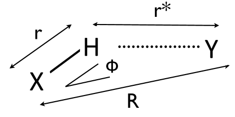
Figure 1: Definition of geometric variables for a hydrogen bond between a donor (X) and an acceptor (Y). This paper is concerned with the quantum motion of the proton H relative to X and Y. The focus in on the case of linear bonds where $\phi=0$ and $r^{*}=R-r$. The quantum effects are largest when the donor-acceptor distance $R$ is about $2.4-2.5$ Å.

II A simple model for ground state potential energy surfaces

This is based on recent work by one of us McKenzieCPL . We briefly review the underlying physics and chemistry behind the simple effective Hamiltonian which produces the potential energy surfaces that we use to describe the nuclear motion.

II.1 Reduced Hilbert space for the effective Hamiltonian

Diabatic states PacherJCP88 , including valence bond states, are a powerful tool for developing chemical concepts Shaik . It has been proposed in many earlier works that hydrogen bonding and hydrogen transfer reactions can be described by an Empirical Valence Bond (EVB) model Horiuti ; CoulsonAF54 ; Warshel ; BorgisJMS97 ; SagnellaJCP98 ; FlorianJPCA02 involving valence bond states. In the present case, the reduced Hilbert space has a basis consisting of two diabatic states that can be denoted as $\left|\text{X-H}^{+},\text{Y}\right\rangle$ and $\left|\text{X},\text{H-Y}^{+}\right\rangle$. The latter represents a product state of the electronic states of an isolated X molecule and of an isolated Y-H⁺ molecule. The difference between the two diabatic states is transfer of a proton from the donor to the acceptor. Note that the positive charges in this notation are nominal, only indicating the presence of the transferring proton on X or Y. The total charge on each of X-H and Y-H would, of course, depend on the charges of X and Y themselves. The X-H and H-Y bonds have both covalent and ionic components, the relative weight of which depends on the distances $r$ and $r^{*}$, respectively. To illustrate these diabatic states we consider three specific examples.

1. For the Zundel cation, (H₅O₂)⁺, a proton is transferred between two water molecules, X$\,=\,$Y$\,=\,$H₂O. The two diabatic states are $|$H₃O⁺, H₂O$\rangle$ and $|$H₂O, H₃O${}^{+}\rangle$ which are degenerate.

2. For the (H₃O₂)^- ion, a proton is transferred between two hydroxide anions: X$=\,$Y$=\,$OH^-. The two diabatic states are $|$H₂O, OH^-$\rangle$ and $|$OH^-, H₂O$\rangle$, which are degenerate.

3. Hydrogen bonding between two water molecules, can viewed in terms of proton transfer between a water molecule and a hydroxide anion: X$=$ OH^- and Y$\,=\,$H₂O, and so this is an asymmetric case. The two diabatic states are $|$H₂O, H₂O$\rangle$ and $|$OH^-, H₃O${}^{+}\rangle$, which are non-degenerate. A very crude estimate of the energy difference between these two states, neglecting significant solvation effects present in aqueous solution, is the free energy difference 21 kcal/mol corresponding to an equilibrium constant of $10^{-14}$.

In this paper, we focus solely on the the symmetric case where the donor and acceptor have the same proton affinity.

II.2 Effective Hamiltonian

The Hamiltonian for the two diabatic states has matrix elements that depend on the X-H bond length $r$, the donor-acceptor separation $R$, and the angle $\phi$, which describes the deviation from linearity (compare Figure 1). It was recently shown that one can obtain both a qualitative and semi-quantitative description of hydrogen bonding using a simple and physically transparent parametrisation of these matrix elements McKenzieCPL . This approach unifies H-bonding involving different atoms and weak, medium, and strong (symmetrical) H-bonds.

The Morse potential describes the energy of a single bond within one of the molecules in the absence of the second (and thus the diabatic states). A simple harmonic potential is not sufficient because the O-H bond is highly anharmonic and we will be interested in regimes where there is considerable stretching of the bonds. The two cases $j=$X, Y denote the donor X-H bond and acceptor Y-H bond, respectively. The Morse potential is

$$V_{j}(r)=D_{j}\left[e^{-2a_{j}(r-r_{0j})}-2e^{-a_{j}(r-r_{0j})}\right],$$ (1)

where $D_{j}$ is the binding energy, $r_{0j}$ is the equilibrium bond length, and $a_{j}$ is the decay constant. $D_{X}$ and $D_{Y}$ denote the proton affinity of the donor and the acceptor, respectively. For O-H bonds, approximate parameters are $D\simeq 120$ kcal/mol, $a\simeq 2.2$ Å^-1, $r_{0}\simeq 0.96$ Å, which correspond to an O-H stretch harmonic frequency, $\omega$, of $\simeq 3750$ cm^-1.

We take the effective Hamiltonian describing the two interacting diabatic states to have the form

$$H=\left(\begin{array}[]{cc}V_{X}(r)&\Delta_{XY}(R,\phi)\\[5.69054pt] \Delta_{XY}(R,\phi)&V_{Y}(r^{*})\end{array}\right),$$ (2)

where

$$r^{*}=\sqrt{R^{2}+r^{2}-2rR\cos\phi}$$ (3)

is the length of the Y-H bond (see Figure 1). The diabatic states are coupled via the off-diagonal matrix element

$$\Delta_{XY}(R,\phi)=\Delta_{1}\cos\phi\frac{(R-r\cos\phi)}{r^{*}}e^{-b(R-R_{1})}$$ (4)

(see Figure 1), and $b$ defines the decay rate of the matrix element with increasing $R$. $R_{1}$ is a reference distance that we take as $R_{1}\equiv 2r_{0}+1/a\simeq 2.37$ Å. This is introduced so that the constant $\Delta_{1}$ sets an energy scale that is physically relevant. The functional dependence on $R$ and $\phi$ can be justified from orbital overlap integrals MullikenJCP49 together with a valence bond theory description of four-electron three-orbital systems (see page 68 of Ref. Shaik, ). There will be some variation in the parameters $\Delta_{1}$ and $b$ with the chemical identity of the atoms (e.g. O, N, S, Se, …) in the donor and acceptor that are directly involved in the H-bond.

II.3 Parametrisation of the diabatic coupling

Since the Morse potential parameters are those of isolated X-H and Y-H bonds, the model has essentially two free parameters, $b$ and $\Delta_{1}$. These respectively set the length and energy scales associated with the interaction between the two diabatic states. That only two parameters are used here is in contrast to most multi-parameter EVB models and empirical ground state potential energy surfaces Korth . For example, one version of the latter involves 11 parameters for symmetric bonds and 27 parameters for asymmetric bonds LammersJCC07 . A significant point of Ref. McKenzieCPL, was that just the two parameters, $b$ and $\Delta_{1}$, are sufficient to obtain a semi-quantitative description of a wide range of experimental data for a chemically diverse set of complexes. The parameter values that are used here, $\Delta_{1}=0.4D\simeq$ 2 eV and $b=2.2$ Å^-1 for O-H$\cdots$O systems, were estimated from comparisons of the predictions of the model with experiment McKenzieCPL .

II.4 Potential energy surfaces

In the adiabatic limit, the electronic energy eigenvalues of Eq. (2) for linear bonds ($\phi=0$) are the eigenvalues of the effective Hamiltonian matrix:

$$\epsilon_{\pm}(r,R) = \tfrac{1}{2}\left[V_{X}(r)+V_{Y}(R-r)\right]$$ (5)

$$\pm\tfrac{1}{2}\left[(V_{X}(r)-V_{Y}(R-r))^{2}+4\Delta(R)^{2}\right]^{\frac{1}{2}}.$$

In this paper, we focus on the case of symmetric bonds where the parameters in $V_{X}$ and $V_{Y}$ are identical.

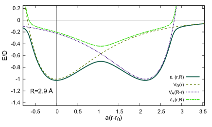
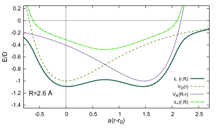
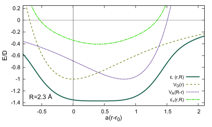
Figure 2: Potential energy curves for the diabatic and adiabatic states of a symmetric hydrogen bonded system. The horizontal axis is proportional to the extent of stretching of the X-H bond. The vertical energy scale is $D$, the binding energy of an isolated X-H bond. The adiabatic curves are for an off-diagonal coupling with parameters $\Delta_{1}=0.4D$ and $b=a$. The diabatic curves are Morse potentials centred at $r=r_{0}$ (dashed lines) and $r^{*}=R-r_{0}$ (dotted lines) and correspond to isolated X-H and H-Y bonds, respectively. For parameters relevant to a O-H$\cdots$O system, the three sets of curves correspond (from top to bottom) to oxygen atom separations of $R=2.9$, 2.6, and 2.3 Å, respectively, characteristic of weak, moderate (low barrier), and strong hydrogen bonds Gilli09 . Note that the upper two panels differ from the corresponding figure in Ref. McKenzieCPL due to an error in that work.

Figure 2 shows the eigenvalues (potential energy curves) $\epsilon_{-}(r,R)$ and $\epsilon_{+}(r,R)$ as a function of $r$, for three different fixed $R$ values. These are three qualitatively different curves, corresponding to weak, moderate, and strong hydrogen bonds, and are discussed in more detail below. [Note that Figure 2 of Reference McKenzieCPL, contained an error in the plots of the potential energy curves and so the corrected curves are shown here.] The surface $\epsilon_{+}(r,R)$ describes an electronic excited state, and should be observable in UV absorption experiments McKenzieCPL . This excited state is seen in quantum chemical calculations for the Zundel cation Geru .

III Vibrational eigenstates

Under the Born-Oppenheimer approximation, the nuclear dynamics is determined by the adiabatic electronic ground state potential energy, $\epsilon_{-}(r,R)$. We numerically solve the one-dimensional Schrödinger equation for motion of a nucleus (proton or deuteron) of reduced mass $M$ in this potential $\epsilon_{-}(r,R)$ for different fixed donor-acceptor distances $R$,

$$\left(-{\hbar^{2}\over 2M}{d^{2}\over dr^{2}}+\epsilon_{-}(r,R)\right)\Psi_{n}(r)=E_{n}\Psi_{n}(r),$$ (6)

to find the low-lying vibrational eigenstates $\Psi_{n}(r)$ and energy eigenvalues $E_{n}$. Isotope effects arise because the solutions depend on $M$ (see note reduced ). Two different numerical methods were used in order to check the results, viz. the Discrete Variable Representation (DVR)Miller ; Groenenboom with a basis of sinc-functions, and the FINDIF program Glendening .

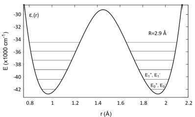
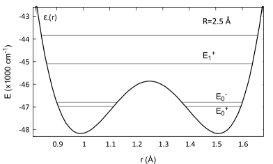
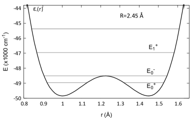
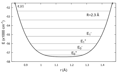
Figure 3: Evolution of the potential energy curve and the vibrational energy levels with decreasing donor-acceptor distance $R$, from top to bottom. This variation corresponds to changing from weak to moderate to strong symmetric bonds. The energy levels shown are for protons. Note that for $R>2.6$ Å, the tunnel splitting between the two levels localised on opposite sides of the potential barrier is not visible. In contrast, at shorter $R$, the zero-point energy becomes comparable to the barrier height and the tunnel splitting between the two lowest levels becomes visible. Note that the horizontal and vertical scales of the above graphs are slightly different from one another.

Figure 3 illustrates how the vibrational energy eigenvalues vary as the donor-acceptor distance $R$ is varied. There are three qualitatively distinct regimes:

1. Weak bonds ($R>2.6$ Å)
   There is a large potential barrier, and so the tunnel splittings are a small fraction of the energy spacings. They are not visible for any of the levels on the scale of the plot shown for $R=2.9$ Å in Figure 3. Nevertheless, in the gas phase small tunnel splittings have been observed for malonaldehyde (26 cm^-1) and tropolone (1 cm^-1) and their derivatives Redington .

2. Low-barrier bonds ($R\simeq 2.4-2.6$ Å)
   The zero-point energy is comparable to (but less than) the potential barrier. There is a visible tunnel splitting of the two lowest levels. The role of such bonds in enzyme catalysis is controversial Cleland ; Warshel96 ; Hosur .

3. Strong bonds ($R\lesssim 2.4$ Å)
   The ground state lies above the barrier or there is no barrier note . All the vibrational energy levels are well-separated.

III.1 Proton probability density

The relevance of the probability density to X-H bond lengths is discussed in the next section. As an aside, we note that the spatial probability density of the ground state, $\rho(r)=|\Psi_{0}(r)|^{2}$, is the Fourier transform of the momentum density $n(p)$ along the direction on of the X-H bond. A directional average of this quantity can be measured by deep inelastic neutron scattering Mayers . The momentum probability density has been observed for a wide range of systems including liquid water, ice, supercooled water, water confined in silica nanopores Garbuio , water at the surface of proteins Pagnotta , water bound to DNA Reiter10 , water inside carbon nanotubes Reiter06 , the ferroelectric KH₂PO₄ Reiter02 , hydrated proton exchange membranes Reiter12 , and a superprotonic conductor Rb₃H(SO₄)₂ Homouz .

For all the radial distributions, $p^{2}n(p)$ has a peak for $p\sim 7$ Å^-1. However, with the exception of Rb₃H(SO₄)₂, liquid water, and ice, a shoulder or second peak is seen at larger momentum, $p\sim 15-20$ Å^-1. Taking the Fourier transform leads to a real-space ground state probability density that is bimodal, as a result of the second peak. It can be fitted with two Gaussians with peaks about $0.2-0.3$ Å apart. Furthermore, with knowledge of the average kinetic energy and the probability density one can construct an effective one-body one-dimensional potential energy for the motion of the proton along the hydrogen bonding direction. For the bimodal distributions the potential is a double well, whereas for the superprotonic conductor it is narrow single well Homouz .

These experimental results can be compared to the one-dimensional potentials and ground state wave functions that we present here. The comparison suggests that in the systems with bimodal distributions that there is some fraction of the water molecules that are sufficiently close that the oxygen-oxygen distance is about $2.4-2.5$ Å. For reference, in bulk water this distance is about $2.8-2.9$ Å. However, it is possible the water molecules could be forced closer to one another due to the interaction of the water with the relevant surface via bonding to the surface or by making the water acidic or basic [producing H₅O${}_{2}^{+}$ or H₃O${}_{2}^{-}$ units]. Indeed, both effects occur for water-hydroxyl overlayers on transition metal surfaces LiPRL10 . However, atomistic simulations of some of these specific systems [e.g., water in silica pores Gallo ] do not seem to produce this effect.

The probability density has been calculated for various phases of water by path integral techniques by Morrone, Lin, and Car, using potential energy functions from electronic structure calculations based on density functional theory MorroneJCP . For water, they considered three different donor-acceptor distances of 2.53, 2.45, and 2.31 Å, corresponding to three different high pressure phases of ice, VIII, VII, and X, respectively. In Ref. MorroneJSP, these results have been interpreted in terms of a simple empirical one-dimensional model potential. But it was also suggested that a single proton distribution is problematic due to proton correlations such as those associated with the “ice rules”. Perhaps such effects could be treated here in a rather limited fashion by allowing for donor-acceptor asymmetries.

IV Bond lengths

Classically, the X-H bond length is simply defined by $r_{min}$, the minimum in the ground state potential energy. However, if the quantum motion of the proton is taken into account, there are ambiguities in defining the bond length that is measured in a neutron scattering experiment. Presumably, this bond length is some sort of motional average associated with the ground state probability density. One possibility, then, is to define the bond length by $r_{max}$, the maximum in the probability density (square of the wave function) for the proton. If the potential energy is not symmetric about the minimum, as is the case here, the maximum of the probability density does not correspond to the minimum of the potential energy; this difference has been pointed out previously by Sokolov, Vener, and Saval’ev Sokolov1 . These two different definitions of the X-H bond length are illustrated in Figure 4 for moderate-to-strong bonds.

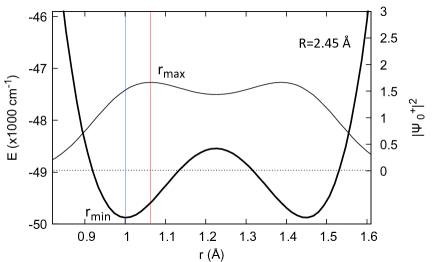
Figure 4: Two definitions of the X-H bond length. One is $r_{min}$, the minimum of the ground state adiabatic potential, a classical definition, shown as a blue vertical line. The other, $r_{max}$, shown as a red vertical line, is the maximum of the ground state vibrational probability density (right-hand scale), which accounts for the quantum vibrational zero-point motion in the anharmonic and asymmetric (about $r_{min}$) ground state potential. The plot is for $R=2.45$ Å, which falls in the moderate-to-strong hydrogen bond range. The dotted horizontal line is the zero-point energy.

Figure 5 shows how quantum nuclear motion significantly shifts $r_{max}$ (red solid line for the hydrogen and blue dashes for the deuterium) from $r_{min}$ (green dot-dashes) as a function of the donor-acceptor distance. The blue crosses are experimental data in Figure 6 of Ref. GilliJACS94, for O-H$\cdots$O bonds in a wide range of crystal structures. A useful length scale for comparison is the zero-point amplitude of an isolated X-H bond vibration, which is about 0.1 Å for O-H bonds with ca. 3600 cm^-1 harmonic frequencies. Relative to this metric, the two bond length definitions give distinct trends in Figure 5; the $r_{max}$ curve corresponds more closely to the measured X-H bond lengths. For the moderate-to-strong H-bonds that occur for $R\lesssim 2.5$ Å, $r_{max}$ increases more sharply because the energy barrier becomes comparable to the zero point energy. Furthermore, there are significant primary geometric isotope effects in the same $R$ range, i.e. the $r_{max}$ traces are significantly different for hydrogen and deuterium. In subsequent sections, $r_{max}$ is referred to as the X-H bond length.

We note that similar curves to those shown in Figure 5 were produced from ab initio path integral calculations for ice under pressure BenoitNature . In particular, the transition to symmetric bonds for $R<2.4$ Å was identified with the experimentally observed transition to ice X for pressures above 62 GPa for H₂O and 72 GPa for D₂O Pruzan . Similar empirical curves including the correction due to quantum zero-point motion have been presented for both oxygen [O-H$\cdots$O] and nitrogen systems [N-H$\cdots$N] by Limbach and collaborators LimbachJMS04 ; Limbach09 .

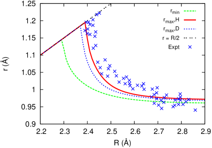
Figure 5: Correlation between the X-H bond length $r$, defined in two ways, and the X-Y distance $R$. The green dot-dashed curve, $r_{min}$, is the classical bond length (minimum of the adiabatic ground state potential; see Figure 4). The solid red and blue dashed curves are the bond lengths are maxima of the ground state probability distribution for the hydrogen and deuterium vibrational wavefunctions, respectively; see Figure 4. The blue crosses are experimental data for O-H$\cdots$O bonds in a wide range of crystal structures, and are taken from Figure 6 in Ref. GilliJACS94, . The black dotted line corresponds to symmetric H-bonds ($r=R/2$) that occur when the potential has a single minimum.

V Longitudinal vibrational frequencies

There is some subtlety in using the calculated vibrational energy levels to deduce the vibrational frequency that is actually measured in an infra-red spectroscopy experiment. A good quantum number is the parity of the vibrational energy level, associated with inversion symmetry about $r=R/2$ in the potentials shown in Figure 3. Each pair of tunneling-split levels have opposite parity, and can therefore be labelled $0^{+}$, $0^{-}$, $1^{+}$, $1^{-}$, … (following the case of the umbrella inversion mode in ammonia Glendening ). The transition dipole operator has odd parity, which, coupled with room or lower temperature Boltzmann weights of the vibrational energy levels, suggest that the relevant transitions are $0^{-}\rightarrow 1^{+}$ and $0^{+}\rightarrow 0^{-}$.

Figure 6 compares the frequencies of both transitions from our calculations with experimental data. As the donor-acceptor distance decreases, there is a significant softening in the experimental X-H stretch frequency (blue crosses) Novak ; Gilli09 ; SteinerACIE ; Libowitzky ; Sikka ; caveat , a trend that is largely traced by the $0^{-}\rightarrow 1^{+}$ energy gap (green solid line). This softening has been proposed as a measure of the strength of an H-bond LiPNAS11 . The harmonic limit, i.e. the frequency obtained from the curvature with respect to $r$ at the bottom of the potential $\epsilon_{-}(r,R)$, is larger in value, and an increasingly poor estimator of transition frequencies with increasing anharmonicity (decreasing $R$) harmonic .

The $0^{+}\rightarrow 0^{-}$ (red dot dashed line) transition is of relevance only at $R\lesssim 2.5$ Å. For $R\gtrsim 2.55$ Å, the $0^{+}\rightarrow 0^{-}$ frequency may not be realistically observable in a condensed phase because the environment will decohere the system and suppress tunneling Weiss .

For $R\approx 2.45$ Å, there are some experimental data points that lie between the two continuous theoretical curves. We consider three possible reasons for this discrepancy. First, the one-dimensional potential may be unreliable in this regime. However, we consider this unlikely because the potential appears to successfully describe so many other properties [bond lengths, geometric and frequency isotope effects]. Second, the two-dimensional character of the potential becomes important [i.e., the coupling of X-H stretch with the X-Y stretch]. Third, there is significant uncertainty in the experimental values for the frequency in this regime. IR spectra for such strong H-bonded complexes in this frequency range are broad (compare Figure 2 in Reference Novak, ) and it is difficult to identify the appropriate vibrational frequency Grdadolnik . This large width is due to the combined effects of the large thermal and quantum fluctuations in $R$ (compare Figure 6 in Ref. Pirc2010, ) and the fact that the stretch frequency varies significantly with $R$.

The present results are relevant to infra-red spectra measured for ice under high pressures, including the symmetric phase, Ice X goncharov ; aoki . Two vibrational modes are seen. These can be identified with the curves for $E_{1^{+}}-E_{0^{-}}$ and $E_{0^{-}}-E_{0^{+}}$ shown in Figure 6. Some caution is in order in making a quantitative comparison because water does not have a symmetric donor and acceptor for hydrogen bonding.

For the rest of this manuscript, we refer to the $0^{-}\rightarrow 1^{+}$ transition frequency as the X-H stretch frequency, $\Omega$.

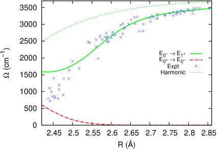
Figure 6: Softening of the X-H stretch frequency $\Omega$ (in cm^-1) with decreasing donor-acceptor distance $R$ (in Å). The green dashed curve is the harmonic frequency at the $r_{min}$ of $\epsilon_{-}(r,R)$. The red dot-dashed curve is the energy difference ($E_{0^{-}}-E_{0^{+}}$) between the two lowest lying energy levels (tunnel splitting of the ground state). The green solid curve is the energy difference ($E_{1^{+}}-E_{0^{-}}$) between the first and second excited state energy levels. The blue crosses are experimental data for a wide range of complexes, and are taken from Figure 4 in Ref. SteinerACIE, .

VI Isotope effects

VI.1 Secondary geometric isotopic effects

Figure 5 and Section IV discuss the primary geometric isotope effects where the X-H bond length changes upon substitution of the hydrogen with deuterium. Secondary effects are those where the X-Y bond length changes, and are also known as the Ubbelöhde effect Ubbelohde . There have been extensive experimental HamiltonAC63 ; LimbachJMS04 ; Limbach09 ; Ip12 ; Madsen07 and theoretical LiPNAS11 ; Ichikawa ; Saitoh ; Tanaka ; Sokolov1 ; Sokolov ; Swalina ; Vener07 ; Koval02 ; YangCPL ; YangZPC investigations of these geometric isotope effects.

The secondary geometric isotope effect complicates the interpretation of other isotope effects. Since the $R$ value changes between the isotopes, the effective one-dimensional potential for each of them is different. Therefore, the shifts due to the primary isotope effect are further modified. This convolution of geometric isotope effects is seen by comparing the crystal structure of CrHO₂ and CrDO₂; in the former the O-H-O bond appears to be symmetric ($r=R/2$) with $R=2.49\pm 0.02$ Å, whereas the O-D-O bond is asymmetric with an O-D bond length of $0.96\pm 0.04$ Å, with $R=2.55\pm 0.02$ ÅHamiltonAC63 . The shift of $R$ value appears small (a 2% change) for the low frequency motion that represents the X-Y stretch, but the effect is palpable.

Generally, one observes that for moderate H-bonds the equilibrium donor-acceptor distance $R$ increases with substitution of hydrogen with deuterium Ichikawa . This is sometimes referred to as a positive secondary geometric isotope effect. For strong bonds, a negative effect, i.e., decrease of $R$, is observed. For weak bonds, $R$ decreases, and understanding this requires inclusion of the transverse vibrational modes LiPNAS11 ; Swalina , as discussed in Section VII.

We now consider a simple extension to our model potential in order to describe the secondary geometric isotope effect for strong to moderate bonds. We draw from the model studies by Sokolov, Vener, and Saval’ev Sokolov1 . Consider a two-dimensional potential in terms of $r$ and $R$. This will contain an attractive (with respect to $R$) contribution from the H-bond [$\epsilon_{-}(r,R)$ in our model] as well as a repulsive term associated with the donor-acceptor repulsion repulsion [so far not included in our model]. Competition between these two contributions determines the classical donor-acceptor bond length, here denoted $R_{0}$. Such a two-dimensional potential would be the same for hydrogen and deuterium. Here we may carry out a Born-Oppenheimer-like treatment of $r$ and $R$. Upon taking an expectation value with the ground state vibrational wavefunction along the fast coordinate, $r,$ an effective one-dimensional potential along $R$ is obtained with the following form:

$$U_{0}(R)=U(R_{0})+{K(R_{0})\over 2}(R-R_{0})^{2}+Z(R),$$ (7)

where the first two terms on the right-hand side are a local quadratic expansion about the $R_{0}$, and represent the elastic modulation of energy along the donor-acceptor stretching coordinate. The essential physics of the isotope effect is in the third term, the zero-point energy,

$$Z(R)\equiv E_{0^{+}}(R)-\epsilon_{-}(r_{min},R),$$ (8)

of the hydrogen (deuterium) motion.

Note that $Z(R)$ is not required to be a minimum at $R_{0}$. Minimising the total energy (7) as a function of $R$ gives the equilibrium bond length

$$R_{eq}=R_{0}-{1\over K(R_{0})}{dZ(R_{0})\over dR}$$ (9)

to first order in $\hbar$ correction . This equation was previously presented by Sokolov, Vener, and Saval’ev Sokolov1 . They used zero-point energies obtained from different model potentials to that used here, and they also assumed that $K(R)$ was constant. The physics involved is identical to that used in solid state physics to calculate the effect of isotope substitution on the lattice constant of a crystal Allen ; Pamuk .

We estimate $K(R_{0})$, the elastic constant in the above model, from experimental information in the article by Novak (Ref. Novak, , Figure 10 and Table V). It shows significant variation with $R_{0}$, increasing by a factor of about 6 as $R_{0}$ decreases from 2.7 to 2.44 Å. The data fits an exponential form,

$$K(R_{0})=\bar{K}\exp\left[-c(R_{0}-\bar{R}_{0})\right],$$ (10)

with $\bar{K}=(55\pm 3)\times 10^{3}{\rm cm}^{-1}/\text{\AA}^{2}$, and $c=(7.3\pm 0.8)$ Å^-1, and $\bar{R}_{0}\equiv 2.5$ Å.

The zero-point energy of the X-H stretch is a non-monotonic function of $R$. The significant variation with $R$ reflects the qualitative changes in the one-dimensional potential that occur as one changes from weak to moderate to strong bonds (compare Figure 3). Furthermore, there are subtle differences between hydrogen and deuterium isotopes. The top part of Figure 7 shows a plot of the slope $dZ/dR$ versus $R$ for both hydrogen and deuterium. This slope is small and positive for large $R$, increases as $R$ decreases until it reaches a maximum for $R\simeq 2.45$ Å for hydrogen ($R\simeq 2.40$ Å for deuterium), becomes zero for $R\simeq 2.33$ Å, and turns negative for smaller $R$.

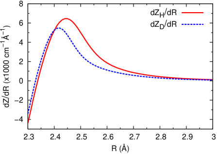
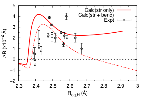
Figure 7: Non-monotonic dependence of the secondary geometric isotope effect on the donor-acceptor distance. The top panel shows the slope of the zero-point energy in cm^-1/Å. The red curve is for hydrogen and the dashed blue curve for deuterium. Note that the maxima occur at different values of $R$ and that the curves cross for $R\simeq 2.4$ Å. The difference between the two curves determines the secondary geometric isotope effect [compare equation (11)] which is shown as the solid curve in the bottom panel. The inclusion of the zero-point contribution of the bend modes, discussed in Section VII and based on results in Ref. McKenzieCPL, , yields the dashed curve in the bottom panel. Experimental data are taken from Table 1 in Ref. Sokolov1, .

With the above pieces of information, the secondary geometric isotope effect is given by

$$\Delta R\equiv R_{eq,\,D}-R_{eq,\,H}={1\over K(R)}\left({dZ_{H}\over dR}-{dZ_{D}\over dR}\right).$$ (11)

In this equation, the $0$ subscript for $R$ has been dropped. $R_{0}$ was used earlier in the section to indicate the classical minimum for various complexes. However, $R$ in the model effectively takes the role of $R_{0}$, scanning through the classical minima of all complexes. The solid curve in the bottom part of Figure 7 (labelled ‘str only’) shows a plot of $\Delta R$ vs $R_{eq,H}$, including a comparison with experimental data from a wide range of complexes, as tabulated in Ref. Sokolov1, .

We point out that the $x$-axis of this plot, obtained from equation (9), is different from $R$, the minimum of the classical potential. For $R\geq 2.35$ Å, we find that $R-R_{eq,H}$ is, like $Z(R)$, a non-monotonic function of $R$. It reaches a maximum value of 0.1 Å for $R\simeq 2.5$ Å, and drops towards zero on either side. Therefore, there is an important difference between plotting the secondary geometric isotope effect versus $R_{eq,H}$ and versus $R$. The former is the most self-consistent approach, since $R_{eq,H}$ is what is experimentally measured. But both approaches produce qualitatively similar results.

The proximity of the theoretical prediction by Eq. (11) to experimental data is encouraging. In particular, the model predicts negative $\Delta R$ values at short donor-acceptor distances (strong H-bonds), though the location of the sign change is slightly offset from experimental data. The fact that the secondary geometric isotope effect becomes negative (and small) for strong H-bonds is seen in ab initio molecular dynamics simulations for H₅O${}_{2}^{+}$ Suzuki2013 , H₇N${}_{2}^{+}$ YangCPL , and H₃F${}_{2}^{+}$ Suzuki2012 . For example, for H₅O${}_{2}^{+}$, it is found that at a temperature of 100 K, $R=2.417$ Å and $\Delta R=-0.004$ Å Suzuki2013 .

The value of $R_{eq,H}$ from Eqn. (9), and consequently $\Delta R$, depends on the total zero-point energy, i.e., not just that from the X-H stretch but also from the X-H bends. It was recently noted LiPNAS11 that the influence of the bends is rather pronounced at large X-Y separations ($\simeq 2.7$ Å). The dashed line labelled ‘str+bend’ in the lower panel of Figure 7 is an attempt to include the effect of the zero-point energy of the bending vibrations as well, and is discussed in detail in Section VII.

VI.2 Vibrational frequency isotope effects

The ratio of the frequency of longitudinal X-H stretching mode for hydrogen to deuterium isotopes is observed experimentally to be a non-monotonic function of the X-Y distance with values varying between 0.85 and 2.0 Novak ; Sokolov ; Grech ; sponge . In contrast, for the torsional/bending modes, the isotope effects are trivial. Table 6 of Ref. Novak, shows that as the O$\cdots$O distance increases from 2.44 Å to 2.71 Å, the ratio of the O-H to O-D (out of plane) bend frequencies vary little, lying in the range 1.32-1.44, and show no significant trend. Broadly, they are consistent with the semi-classical harmonic ratio $\sqrt{2}$. This is expected since for the bending mode there is no significant anharmonicity (compared to the stretch mode). With respect to the $\phi$ co-ordinate in Figure 1, hydrogen bonding simply hardens the potential for non-linear arrangements.

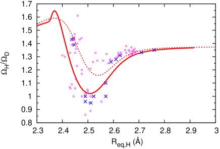
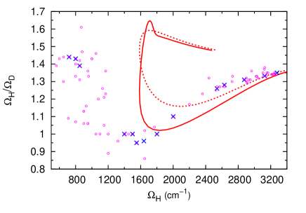
Figure 8: Top panel: Correlation between the frequency isotope effect and the donor-acceptor distance $R_{H}$, of the hydrogen isotope. The vertical axis is the ratio of the O-H stretch frequency to the O-D stretch in the same compound. The solid curve is $\Omega_{H}(R_{H})/\Omega_{D}(R_{D})$ (i.e., the two frequencies are calcuated for different one-dimensional potentials) whereas the dashed curve is the frequency ratio calculated at the same distance $R_{H}$ (i.e., for the same potential). The difference between the two curves for $R\sim 2.5$ Å, highlights the contribution of the secondary geometric isotopic effect, calculated from equation (11). Bottom panel: The data is the same as in the top panel, but the horizontal axis is $\Omega_{H}$ instead of $R_{H}$. Experimental data in both plots are from Table 6 in Ref. Novak, (crosses) and Table 1 in Ref. Sokolov, (open circles).

Figure 8 compares the calculated correlation between the frequency isotope effect with the donor-acceptor distance for the hydrogen isotope for a wide range of complexes. It is particularly striking that if one simply calculates the frequencies for hydrogen and deuterium isotopes at the same donor-acceptor distance [i.e., with the same one-dimensional potential] one does not obtain quantitative agreement with the experimental data for $R_{eq,H}\simeq 2.4-2.5$ Å (compare the dashed curve in Figure 8). Instead, one needs to take into account the secondary geometric isotope effect and calculate $\Omega_{D}$ at $R=R_{eq,D}$, given by equation (11) and plotted in Figure 7 (lower panel, solid curve). For $R_{eq,H}\simeq 2.4-2.5$ Å, the secondary geometric isotope effect is largest, $\Delta R\simeq 0.03$ Å. Although this change in value is small relative to $R$, it makes sufficient alterations in the one-dimensional potential along $r$ for deuterium so that $\Omega_{D}(R_{eq,D})$ becomes comparable to $\Omega_{H}(R_{eq,H})$ (their ratio is closer to 1). Previously, Romanowski and Sobczyk Romanowski calculated a curve similar to the dashed one shown in Figure 8 and suggested that the discrepancy with the experimental data may be due to a change in the potential associated with the secondary geometric isotope effect. We have shown that this is indeed the case. We also note that the horizontal axis $R_{eq,H}$ is given by equation (9).

The $\Omega$ value for both isotopes are calculated as $E_{1^{+}}-E_{0^{-}}$ energies. At short O$\cdots$O distances $\lesssim 2.5$ Å, the $E_{0^{-}}-E_{0^{+}}$ (ground state tunneling splitting) frequencies also enter the range of the experimental data. However, the ratio of these frequencies for hydrogen and deuterium lie above 1.5 (not shown), and thereby above the available experimental data for O-H$\cdots$O. However, experimental data for the frequency ratio of N-H$\cdots$N systems does increase up to 2 for short bonds Grech .

An alternate way of examining the isotope effects with the same data is with a plot of the ratio $\Omega_{H}/\Omega_{D}$ against $\Omega_{H}$ rather than $R_{eq,H}$ Novak ; Sokolov ; Grech . This is done in the lower panel of Figure 8. The present model’s predictions without (dashed curve) and with (solid curve) secondary geometric isotope effect corrections, deviate significantly from the experimental plot, with particularly strong deviations for $R_{eq,H}\lesssim 2.5$ Å, where the frequency ratio turns upward for $\Omega_{H}\simeq 1700\ {\rm cm}^{-1}$ . Note, however, that continuous curves do capture the range of the frequency ratios, just as they do in the upper panel of the figure. The discrepancy is due in part to $\Omega_{H}$; it does not take on values as low as reported in experiments for $R\lesssim 2.5$ Å, an observation noted previously for Fig. 6. In effect, the H-bond potential model in this work is able to recover frequency ratios rather well, but not the experimental frequencies in certain strong H-bonding regions. Then again, the experimental frequencies in this range are difficult to unambiguously identify; see Section V above as well as Refs. Grdadolnik, and Pirc2010, .

VI.3 Simple models for frequency isotope effects

Some insight can be gained into the variation of the isotope effects with the donor-acceptor distance by considering analytical results for simple model potentials that are relevant in different limits.

1. Harmonic potential
   This approximately describes weak hydrogen bonds. For a potential $V(r)=A(r-r_{0})^{2}/2$, the energy eigenvalues are $E_{n}=(n+1/2)\hbar\sqrt{A/M}$. Hence, the frequency $\Omega\equiv(E_{1}-E_{0})/\hbar$. The ratio of the frequencies for hydrogen and deuterium is

   $${\Omega_{H}\over\Omega_{D}}=\sqrt{2}=1.41.$$ (12)

   For weak bonds the anharmonicity factor is small enough ($\chi\sim 0.03$ in equation 13 below) that the above ratio is a reasonable approximation.

2. Morse potential
   This approximately describes the anharmonicity associated with (parameterized around) the bottom of the potential for moderate to weak hydrogen bonds. This is not to be confused with the Morse potential that we use to describe the diabatic states. For a Morse potential, the eigenvalues are $E_{n}=(n+\tfrac{1}{2})\hbar\omega_{0}-(n+\tfrac{1}{2})^{2}\hbar\omega_{0}\chi,$ where $\omega_{0}$ is the harmonic frequency and $\chi\equiv\hbar\omega_{0}/4D_{0}$ is the anharmonicity. The transition frequency is then $\Omega=(E_{1}-E_{0})/\hbar=\omega_{0}(1-2\chi)$. The ratio of the hydrogen and deuterium frequencies is

   $${\Omega_{H}\over\Omega_{D}}=\sqrt{2}\left({1-2\chi}\over{1-{\sqrt{2}\chi}}\right).$$ (13)

   Hence, as $R$ decreases, we expect the frequency ratio to decrease as is observed. Even for large anharmonicity ($\chi\sim 0.2-0.25$), the ratio only decreases to about 1.1-1.2, as is observed in the full calculation (compare the dashed curve in the upper panel of Figure 8).

3. Infinite square well potential
   For strong bonds, the potential is approximately a square well of width $L=R-2r_{0}$. This observation was pointed out in References Horbatenko, and Belot, . For a well of width $L$, the energy of the $n$-th level is

   $$E_{n}={\hbar^{2}n^{2}\over 2ML^{2}}$$ (14)

   where $n=1,2,3,\cdots$. The ratio of the frequencies for the two isotopes is then

   $${\Omega_{H}\over\Omega_{D}}=2.$$ (15)

The detailed calculations of the isotope frequency ratio shown in Figure 8 are consistent with the above three limits. As $R$ decreases, $\Omega_{H}/\Omega_{D}$ decreases below 1.4 reaches a minimum, and then for $R$ values corresponding to a single well potential the ratio increases to values larger than $1.4$.

The ground state wave function for the infinite square well is ($n=1$)

$$\Psi_{g}(r)=\sqrt{2\over L}\sin\left({\pi r\over L}\right),$$ (16)

which is independent of the mass $M$. Hence, the zero-point energy depends on $1/M$, but the zero-point motion is independent of $M$. This is in contrast to the case of a harmonic potential for which the zero-point wavefunction does have $M$ dependence. Indeed, this explains why calculations of the ground state probability distribution $|\Psi_{g}(r)|^{2}$ for the protonated ammonia dimer N₂H${}_{7}^{+}$ YangCPL , for H₃O${}_{2}^{-}$ YangZPC , and for sodium bihydrogen bisulfate Pirc2010 found virtually identical probability distributions for both isotopomers.

The non-monotonic dependence of the zero-point energy $Z(R)$ on $R$ (compare the upper panel of Figure 7) can also be understood in terms of the analytic limits discussed above. As $R$ decreases the potential gets more anharmonic and the zero-point energy $Z=E_{0}=\tfrac{1}{2}\hbar\omega_{0}(1-\hbar\omega_{0}/8D_{0})$ decreases because the effective $D_{0}$ of the local Morse potential also decreases. However, in the single well regime, $Z(R)\sim 1/(R-2r_{0})^{2}$, and the zero-point energy increases with decreasing $R$.

VII Competing quantum effects

There is a torsional or bending vibration associated with periodic oscillation of the angle $\phi$ shown in Figure 1. This is related to the libration mode in water and ice. The bending vibrations make an important contribution to the total zero-point energy of the system [compare equations (7) and (17) below]. As the donor-acceptor distance decreases, the bending frequency and the associated zero-point energy increase (compare Figure 6 in Ref. McKenzieCPL, ). This is the opposite trend to the X-H stretch. These opposite dependences lead to the notion of competing quantum effects Habershon ; Markland ; Romanelli .

In this section, we make a preliminary analysis of the role of H-bond bending on the secondary geometric isotope effects. The total zero-point energy is

$$Z(R)\equiv Z_{\parallel}(R)+Z_{\perp,o}(R)+Z_{\perp,i}(R).$$ (17)

The terms are the zero-point energy associated with X-H vibrations parallel to the hydrogen bond (stretch), out-of-plane bend ($o$), and in-plane bend ($i$) of X-H$\cdots$Y. In the diabatic state model McKenzieCPL , the effect of H-bonding on hardening of the two bend motions is similar,

$$\Omega_{\perp,o/i}(R)^{2}=\omega_{\perp,o/i}^{2}+2f(R)$$ (18)

where $\omega_{\perp,o/i}$ is the frequency in the absence of an H-bond and the function $f(R)$ is given in Eqn. (6) of Ref. McKenzieCPL, . At least in the $R$ range of interest, $f(R)$ is a positive function that monotonically decreases with increasing $R$: $f^{\prime}(R)<0$. In general $\omega_{\perp,i}>\omega_{\perp,o}$ and so $\Omega_{\perp,i}>\Omega_{\perp,o}$. The contributions of the two bending bending modes to the zero-point energy (17) are taken to be $Z_{\perp,o/i}=\tfrac{1}{2}\hbar\Omega_{\perp,o/i}(R)$: they are treated as harmonic oscillators.

The frequency $\Omega_{\perp,o}(R)$ is taken from (the solid line of) Figure 6 of Ref. McKenzieCPL, . Little data is available for the in-plane bend $\Omega_{\perp,i}(R)$ because the interpretation of experimental data is difficult due to the strong mixing of this mode with others Novak . Hence, we use the following simple analysis to estimate its effect. If we take the derivative of Eqn. (18) with respect to $R$ we obtain,

$$\Omega_{\perp,o}\frac{d\Omega_{\perp,o}}{dR}=\Omega_{\perp,i}\frac{d\Omega_{\perp,i}}{dR}={df\over dR}.$$ (19)

Hence, we can write the derivative of the total bend ZPE

$$\frac{dZ_{\perp}}{dR}=\frac{dZ_{\perp,o}}{dR}\left(1+\frac{\Omega_{\perp,o}}{\Omega_{\perp,i}}\right).$$ (20)

It can be seen from equation (18) that $1>\Omega_{\perp,o}(R)/\Omega_{\perp,i}(R)>\omega_{\perp,o}/\omega_{\perp,i}$, and that this frequency ratio progressively increases towards unity as $R$ decreases. Given that information about the out-of-plane bend is known better than the in-plane bend, we make a limiting approximation that $\Omega_{\perp,o}\simeq\Omega_{\perp,i},$ so we can write

$$\frac{dZ_{\perp}}{dR}\simeq 2\frac{dZ_{\perp,o}}{dR}.$$ (21)

This becomes less reliable for larger $R$ (when $f(R)$ becomes smaller), giving an overestimate of the magnitude of the total bend derivative.

All terms in equation (17) vary significantly with $R$ in the range of interest (2.3-3.0 Å). The first term has a non-monotonic trend (as shown in the upper panel of Figure 7), whereas the bend terms decrease monotonically as $R$ is increased. So the total zero-point energy involves a subtle competition between the stretch and bend components at different values of $R$.

The net secondary geometric isotope effect comes from a balance between $\left[dZ_{\parallel,H}/dR-dZ_{\parallel,D}/dR\right]$ for the stretch and $2\left[dZ_{\perp,o,H}/dR-dZ_{\perp,o,D}/dR\right]$ for both bends together (compare equation (11)). Noting that $\Omega_{\perp,o/i}$ scale essentially as the square root of the mass of H or D, the derivative difference for the bends can be simplified to $2\left(1-\tfrac{1}{\sqrt{2}}\right)dZ_{\perp,o,H}/dR$.

At $R\simeq 2.4$ Å and $R\gtrsim 2.7$ Å, the derivative difference for the stretch mode is small; see the upper panel of Figure 7. It is in these regions that the the bend contributions will be particularly noticeable. For example, at 2.4 Å, $dZ_{\perp,o,H}/dR\simeq-800$ cm^-1, so that the derivative difference for both bends together is about $-450$ cm^-1. The secondary geometric isotope effect is negative in sign at this $R$ value, and contains a substantial contribution from the bend.

The dashed line in the lower panel of Figure 7 (labelled ‘str+bend’) gives an estimate of the secondary geometric isotope effect including both bends. The overall features of the change in donor-acceptor distance $\Delta R$ are not too different at short $R$, apart from an overall downward shift. But at $R_{eq,H}\gtrsim 2.7$ Å, the bend contribution overtakes the stretch giving rise to a negative $\Delta R$. The position of the crossover may change slightly with a more refined treatment of the bend modes and the model itself. Specifically, for weak bonds the contribution of the in-plane bend will become smaller than that of the out-of-plane bend (compare Eqn. (20)). Indeed, this difference was also found for path integral simulations of isotopic fractionation in water Markland . Consequently, $\Delta R$ will become negative at a larger $R_{eq,H}$ than the value of about 2.7 Å shown in our Figure 7. At still larger distances, $R_{eq,H}>3.0$ Å, the H-bonding becomes very weak, and it is expected that the $\Delta R$ curve eventually goes to zero.

The qualitative aspect of a negative $\Delta R$ for weak H-bonds is in agreement with recent work of Li et al. LiPNAS11 based on Path Integral Molecular Dynamics simulations. They showed that the bend modes would dominate over the stretch for weak H-bonds, leading to a negative secondary geometric isotope effect at large donor-acceptor distances. They found a change in the sign of the geometric isotope effect when the H-bond strength was such that the X-H stretch frequency was reduced by about 30 per cent. From Figure 6 we estimate this corresponds to $R_{eq,H}\simeq 2.6$ Å, a value somewhat lower than the crossover region we see in Figure 7.

VIII Possible future directions

There are several natural directions to pursue future work. These include the description of asymmetric complexes where the proton affinity of the donor and acceptor are different. As a result the one-dimensional potential is no longer symmetric about $r=R/2$. Development of a full two-dimensional potential $V(r,R)$ will allow treatment of the secondary geometric isotope effect without introducing the empirical elastic constant $K(R)$ and investigating of the coupling of thermal and quantum fluctuations between $R$ and the X-H stretch. This simple diabatic state model approach can be readily be applied to more complex H-bonded systems such as those associated with solvated Zundel cations Reed , excited state proton transfer, double proton transfer in porphycenes Waluk , and water wires Chen . Finally, we briefly discuss two other future directions.

VIII.1 Anisotropic Debye-Waller factors

For crystal structures, one assigns ellipsoids associated with the uncertainty of the positions of individual atoms determined from X-ray or neutron diffraction experiments. The relevant quantities are known as Atomic Displacement Parameters or Debye-Waller factors. In the absence of disorder, their magnitude is determined by the quantum and thermal fluctuations in the atomic positions. Anisotropy in the ellipsoid reflects a directional dependence of bonding and the associated vibrational frequencies. Anisotropy in the associated kinetic energy of protons in liquid water and in ice was recently measured by inelastic neutron scattering Romanelli .

The variation in the anisotropy of the ellipsoid with donor-acceptor distance has been calculated for ice by Benoit and Marx Benoit05 . Anisotropy of the Debye-Waller factor for the position of protons in enzymes has recently been critically examined with a view to identifying low-barrier H-bonds Hosur . The authors found that anisotropy is correlated with the presence of short bonds and with “matching $pK_{a}$’s” [i.e., the donor and acceptor have similar chemical identity and proton affinity], as one would expect.

Our calculations of the variation of X-H stretch zero-point energy with respect to $R$ and the X-H bend frequency (Figure 6 in Ref. McKenzieCPL, ) suggest the anisotropy has a non-monotonic dependence on $R$.

VIII.2 Hamiltonian for non-adiabatic effects

The model Hamiltonian (2) has a natural extension to describe non-adiabatic effects associated with a quantum mechanical treatment of the hydrogen atom co-ordinate $r$. The harmonic limit for symmetric donor and acceptor corresponds to a spin-boson model KoppelACP84 with the quantum Hamiltonian

$$H={\hat{p}^{2}\over 2M}+{M\over 2}\omega^{2}\hat{q}^{2}+\left(\begin{array}[]{cc}g\sqrt{2M\omega}\hat{q}&\Delta(R)\\ \Delta(R)&-g\sqrt{2M\omega}\hat{q}\end{array}\right)$$ (22)

where $\hat{p}$ is the momentum operator, conjugate to $\hat{q}\equiv\hat{r}-R/2$, and $g\equiv\sqrt{M\omega^{3}\over 2}(R/2-r_{0})$. This Hamiltonian can be re-written as

$$H=\Delta\sigma_{x}+g(a^{\dagger}+a)\sigma_{z}+\omega a^{\dagger}a$$ (23)

where $\sigma_{x}$ and $\sigma_{z}$ are Pauli matrices and $a$ and $a^{\dagger}$ are annihilation and creation operators, respectively, associated with the $r$ co-ordinate. This Hamiltonian has an analytical solution in terms of continued fractions PaganelliJPCM06 .

The fully quantum Morse potential has an exact analytical solution and an algebraic representation in terms of creation and annihilation operators Levine . Hence, an algebraic treatment of the quantum version of the model Hamiltonian (2) (i.e. without taking the harmonic limit) may also be possible, because the off-diagonal terms are independent of $r$. Given the quantitative importance of the anharmonicity associated with the Morse potential note this is desirable.

Previous studies McKemmish ; Stanton of the Hamiltonian (23) suggest that the most significant deviations from the Born-Oppenheimer approximation will occur when the bare vibrational frequency $\omega\sim\Delta(R)$ and also the barrier height. This will occur when $R\sim 2.5$ Å.

IX Conclusions

We have clearly shown that the quantum motion of the proton has a significant effect on the properties of H-bonds of strong to moderate strength between symmetric donor (X) and acceptor (Y) groups. A simple one-dimensional potential for the linear transfer path (X-H stretch) of the proton at various donor-acceptor separations ($R$), based on a two-diabatic state model with only a very few parameters, was used for this purpose. The structure of this potential varies from a high-barrier double-well for weak and moderate H-bonds ($R\gtrsim 2.7$ Å) to a single well for strong H-bonds ($R\sim 2.4$ Å). Our analysis of the proton motion on this potential gives qualitative and quantitative descriptions of several correlations as a function of $R$ for O-H$\cdots$O containing materials.

The model’s predictions of the basic properties of hydrogen bonding, viz. X-H bond length variations and vibrational frequency red-shifts, for both hydrogen and deuterium isotopes, compare well with known experimental information over a wide $R$ range. The key additional prediction using a slight extension of the model is that of the secondary geometric isotope, or Ubbelöhde, effect, wherein the donor-acceptor distance is changed due to H to D isotopic substitution.

The Ubbelöhde effect is a quantum effect whose magnitude depends on zero-point energies (ZPEs) in the proton and deuteron’s degrees of freedom. We have shown that the ZPE along the X-H(D) stretch is able to capture the experimental trends for strong H-bonds. The model potential shows qualitative changes for $R\lesssim 2.5$ Å, when the barrier becomes comparable to or lower than the ZPE of the X-H(D) stretch mode. Concomitantly, significant variations in the difference between the X-H and X-D ZPE derivatives with $R$ are observed in our model, which dominates the secondary geometric isotope effect for strong to moderate H-bonds. This effect modulates and, indeed, improves the model’s predictions of the primary geometric isotope effect as well.

In this paper, we have employed mainly one-dimensional quantum calculations along the X-H stretch with the donor-acceptor distance ($R$) as a control parameter. This alone is found to be quite insightful. Of course, higher dimensional quantum treatments that include the X-H bends and $R$ are anticipated to yield a still better quantitative description. Taking a short step in this direction, we have made a preliminary analysis of the effect of the X-H bends in the context of the Ubbelöhde effect. We find, in agreement with other recent works, that their influence is mainly in the moderate to weak H-bond regime, where they begin to overtake the influence of the X-H stretch.