The VIMOS Public Extragalactic Redshift Survey (VIPERS)

Abstract

Aims. Non-uniform sampling and gaps in sky coverage are common in galaxy redshift surveys, but these effects can degrade galaxy counts-in-cells measurements and density estimates. We carry out a comparative study of methods that aim to fill the gaps to correct for the systematic effects. Our study is motivated by the analysis of the VIMOS Public Extragalactic Redshift Survey (VIPERS), a flux-limited survey at $i_{AB}<22.5$ consisting of single-pass observations with the VLT Visible Multi-Object Spectrograph (VIMOS) with gaps representing 25% of the surveyed area and an average sampling rate of 35%. However, our findings are generally applicable to other redshift surveys with similar observing strategies.

Methods. We applied two algorithms that use photometric redshift information and assign redshifts to galaxies based upon the spectroscopic redshifts of the nearest neighbours. We compared these methods with two Bayesian methods, the Wiener filter and the Poisson-Lognormal filter. Using galaxy mock catalogues we quantified the accuracy and precision of the counts-in-cells measurements on scales of $R=5\,h^{-1}{\rm Mpc}$ and $8\,h^{-1}{\rm Mpc}$ after applying each of these methods. We further investigated how these methods perform to account for other sources of uncertainty typical of spectroscopic surveys, such as the spectroscopic redshift error and the sparse, inhomogeneous sampling rate. We analysed each of these sources separately, then all together in a mock catalogue that mimicks the full observational strategy of a VIPERS-like survey.

Results. In a survey such as VIPERS, the errors in counts-in-cells measurements on $R<10\,h^{-1}{\rm Mpc}$ scales are dominated by the sparseness of the sample due to the single-pass observing strategy. All methods under-predict the counts in high-density regions by 20-35%, depending on the cell size, method, and underlying overdensity. This systematic bias is similar to random errors. No method outperforms the others: differences are not large, and methods with the smallest random errors can be more affected by systematic errors than others. Random and systematic errors decrease with the increasing size of the cell. All methods can effectively separate under-dense from over-dense regions by considering cells in the $1^{st}$ and $5^{th}$ quintiles of the probability distribution of the observed counts.

Conclusions. We show that despite systematic uncertainties, it is possible to reconstruct the lowest and highest density environments on scales of $5\,h^{-1}{\rm Mpc}$ at moderate redshifts $0.5\lesssim z\lesssim 1.1$, over a large volume such as the one covered by the VIPERS survey. This is vital for characterising of cosmic variance and rare populations (e.g, brightest galaxies) in environmental studies at these redshifts.

1 Introduction

Large-volume spectroscopic redshift surveys have emerged as the best tool for investigating the large-scale structure of the Universe and, eventually, for constraining cosmological models. Measuring spectroscopic redshifts and angular positions allows us to trace the ${\rm 3D}$ distribution of galaxies and, assuming that they trace the underlying density field, of the matter. Effective constraints on the cosmological model can be obtained by comparing the statistical properties of the galaxy distribution with theoretical predictions. Moreover, the apparent distortions in galaxy clustering induced by peculiar velocities provide a unique observational test for non-standard gravity models as alternatives to dark energy to account for the accelerated expansion of the Universe (e.g. Guzzo et al. 2008). Indeed, setting these types of constraints is one of the main scientific drivers of the VIMOS Public Extragalactic Redshift Survey (VIPERS), an ongoing spectroscopic survey of about 100 000 galaxies at $z\simeq 0.8$ (Guzzo et al. 2014). VIPERS has already achieved this goal (see e.g. de la Torre et al. 2013) using part of the dataset now made available with the first Public Data Release (Garilli et al. 2014).

The effect of peculiar velocities is just one of the reasons that prevent us from observing the full 3D distribution of objects. Other effects, either intrinsic (e.g. Galactic absorption of extragalactic light) or induced by the observational strategy (selecting objects above some flux threshold, measuring spectra only for a subset of potential targets, etc.) and instrumental setup, effectively modulate the spatial distribution of objects. All these effects are potential sources of systematic errors that need to be accurately quantified and accounted for.

The impact of these effects and their correction depend on the characteristics of the dataset, on the kind of systematic effects that need to be corrected for, and on the type of analysis one wishes to perform. One of these observational biases is incomplete sky coverage. Correction for this effect is quite trivial when measuring clustering statistics in configuration space. In the specific case of the VIPERS survey, this has been efficiently done through the extensive use of random samples mimicking the observational biases to estimate the two-point correlation function of different types of galaxies (Marulli et al. 2013; de la Torre et al. 2013).

The types of analysis that are most sensitive to inhomogeneous sky coverage include the study of galaxy properties and their relation to the local environment. Clearly, the presence of unobserved areas with size comparable to the physical scale that one wishes to investigate can have a serious impact on the analysis. In this case a large-scale statistical correction is not sufficient. Instead, a more local and deterministic recovery of the missing information is mandatory (e.g. Cucciati et al. 2006).

The best known example of 3D reconstruction is that of the extragalactic objects behind the Galactic plane where observations are hampered by strong photon absorption. This is a long-lasting issue triggered in the ’90s by the search for the ‘Great Attractor’, a putative large-scale structure responsible for the coherent large-scale flows in our cosmic neighbourhood. The need to fill the so-called Zone of Avoidance not only has triggered a long-term observational programme (see e.g. Kraan-Korteweg 2005) but also the development of techniques able to fill the unobserved regions while preserving the coherence of the large-scale structure. Among these techniques, those more relevant for our work are the cloning, or randomised cloning, of the 3D distribution of objects into unobserved areas (e.g. Yahil et al. 1991; Branchini et al. 1999) and the application of the Wiener Filtering technique (e.g. Lahav et al. 1994).

Here we build on these and other more recently developed and sophisticated techniques, such as ZADE (Kovač et al. 2010) and Poisson-Lognormal Filtering (Kitaura et al. 2010), to tackle the problem of reconstructing the 3D distribution of galaxies in the unobserved regions of a much deeper redshift survey. As anticipated, this analysis is targeted to a specific dataset, VIPERS in this case. We can nevertheless draw some general conclusions from this exercise, since some of the problems we address are indeed of interest for future potential surveys at similar or higher redshift that aim at maximising both volume and sampling.

From the point of view of the angular coverage, VIPERS can be considered as a typical example of a survey in which unobserved areas constitute a sizeable fraction ($\sim 25$%) of the total and are characterised by their regular pattern that reflects the footprint of the spectrograph. Some of the systematic effects, such as the violation of the local Poisson hypothesis in cell counting statistics (Bel et al. 2014), can be amplified by the presence of regular gaps, given the significant fraction of unobserved sky.

We do not limit our analysis to the effect of inhomogeneous sky coverage. All other effects, ranging from sparse, inhomogeneous and clustering-dependent galaxy sampling, radial selection induced by the flux threshold, redshift measurement errors, as well as incompleteness induced by selection criteria, are also folded into our analysis. Again, some of these effects are specific to VIPERS but the dominant ones (sparse sampling and flux limit cut) are quite common to general-purpose surveys that aim at both cosmological and galaxy evolution studies.

The paper’s layout is as follows. In Sect. 2 we describe VIPERS data and the mock galaxy catalogues we use in the analysis. We also list the sources of uncertainties for counts in cells. In Sect. 3 we discuss the methods that we use to fill the gaps, and in Sect. 4 we describe how we perform our analysis (the considered sources of uncertainty included in the different mock catalogues, the kinds of comparison we carry on, and the samples and redshift range we consider). Our results are presented in Sect. 5, and in Sect. 6 we summarise and discuss them. The Appendix gives more details about some specific results. In this work, we use the same cosmology assumed in the dark matter N-body simulation on which our mock galaxy catalogues are based (see Sect. 2.2), i.e. a flat $\Lambda$CDM cosmology with $\Omega_{m}=0.27$, $\Omega_{\Lambda}=0.73$, and $H_{0}=70\,{\rm km\,s}^{-1}{\rm Mpc}^{-1}$. Magnitudes are expressed in the AB system (Oke 1974; Fukugita et al. 1996).

2 Data and mock samples

2.1 Data

The VIMOS Public Extragalactic Redshift Survey (VIPERS) is an ongoing Large Programme aimed at measuring redshifts for $\sim 10^{5}$ galaxies at redshift $0.5<z\lesssim 1.2$. The main scientific drivers of this survey are a robust and accurate measurement of galaxy clustering and of the growth of structure through redshift-space distortions and the study of galaxy properties at an epoch when the Universe was about half its current age.

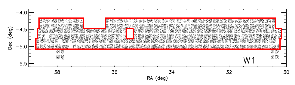
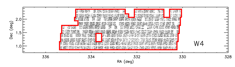
Figure 1: $RA$-$Dec$ distribution of galaxies with reliable redshift (see text for details) in the VIPERS Public Release PDR-1 in W1 (top) and W4 (below) fields. The thick red line in each panel is the ‘field boundary’ that we consider in this work. The VIMOS footprint with four quadrants is visible from the two single pointings at $Dec\lesssim-5.08$ deg in the W1 field at $RA=37.9$ and $RA=30.4$.

At completion, VIPERS will cover $\sim 24$ deg² on the sky, divided into two areas within the W1 and W4 CFHTLS fields. The parent photometric catalogue from which VIPERS targets are selected is the Canada-France-Hawaii Telescope Legacy Survey Wide (CFHTLS-Wide) optical photometric catalogues (Mellier et al. 2008). Galaxies are selected to a limit of $i_{AB}<22.5$, and a colour pre-selection in $(g-r)$ vs $(r-i)$ is also applied to efficiently remove galaxies at $z<0.5$. In combination with an optimised observing strategy (Scodeggio et al. 2009), this allows us to double the galaxy sampling rate in the redshift range of interest with respect to a purely flux-limited sample ($\sim 40\%$). The final surveyed volume will be $5\times 10^{7}$ h^-3 Mpc³, similar to that of the 2dFGRS at $z\sim 0.1$. VIPERS spectroscopic observations are carried out with the VLT Visible Multi-Object Spectrograph (VIMOS, Le Fèvre et al. 2002, 2003), using the LR Red grism (resolution $R=210$, wavelength coverage of 5500-9500$\AA$). The typical radial velocity error is of $\sim 140\,{\rm km\,s}^{-1}$.

A discussion of the survey data reduction and management infrastructure is presented in Garilli et al. (2012), and the complete description of the survey is given by Guzzo et al. (2014). The data set used in this paper represents the VIPERS Public Data Release 1 (PDR-1) catalogue, which was made publicly available in Fall 2013 (Garilli et al. 2014). It consists of $\sim 47000$ galaxies and AGN with reliable spectroscopic redshift. We consider reliable redshifts to be those with spectroscopic quality flag equal to 2, 3, 4, 9 (see Garilli et al. 2014 for a detailed description).

The VIMOS instrument is composed of four CCDs (‘quadrants’) with a field of view of $8^{\prime}\times 7^{\prime}$ each, for a total field of view of $218$ arcmin². The four CCDs are placed on a $2\times 2$ grid with a $2^{\prime}$ separation. The VIMOS pointing footprint is thus characterised by a cross with no data (see below).

As mentioned above, the ‘parent’ photometric catalogue from which targets are selected has a flux limit of $i_{AB}<22.5$ and a colour cut to remove galaxies at $z<0.5$. The consequent cut in redshift is not sharp, but has a smooth transition from $z\sim 0.4$ to $z\sim 0.6$. This has an effect on the radial selection function of the survey. We quantify this effect by the colour sampling rate (CSR from now on). The CSR depends on redshift, and it is equal to 1 for $z\geq 0.6$. Moreover, the VIPERS observational strategy consists in targeting for observations $\sim 40$% of the galaxies in the parent photometric catalogue, and in addition not all the targeted galaxies yield a reliable redshift measurement. All these effects need to be taken into account when deriving the VIPERS selection function. We define the target sampling rate (TSR) as the fraction of galaxies in the parent photometric catalogue that have been targeted, and the spectroscopic success rate (SSR) the fraction of targeted galaxies for which a reliable redshift has been measured. The average VIPERS sampling rate, considering the TSR and SSR together, is $\sim 35$%. The VIPERS sampling rate is not uniform on the surveyed area. Both TSR and SSR depend on VIMOS quadrant. The TSR is higher when the surveyed sky region has a lower target surface density, while the SSR can vary quadrant per quadrant because of different observational conditions. In each quadrant, the number of slits is maximised using the SPOC algorithm (Bottini et al. 2005). We refer the reader to de la Torre et al. (2013) and Fritz et al. (2014) for more details on the VIPERS selection function.

Figure 1 shows the $RA$-$Dec$ distribution of the galaxies and AGN with reliable redshift (see above) in the PDR-1 in the fields W1 and W4. The cross-like pattern of void regions is evident, together with larger empty regions corresponding to quadrants or pointings that have been discarded owing to technical problems or poor observational conditions.

Photometric redshifts ($z_{p}$) were computed for all the galaxies in the photometric catalogue, as described in Coupon et al. (2009) but using CFHTLS T0005 photometry. At $i_{AB}<22.5$, the photometric redshift error is $\sigma_{zp}=0.035(1+z)$, with an outlier fraction of 3-4%. From now on we call ‘spectroscopic galaxies’ the galaxies with a reliable spectroscopic redshift, and ‘photometric galaxies’ all the other galaxies in the parent photometric catalogue having a photometric redshift.

Absolute magnitudes were obtained via spectral energy distribution (SED) fitting technique, using the algorithm Hyperzmass, an updated version of Hyperz (Bolzonella et al. 2000, 2010). We used a template library from Bruzual & Charlot (2003), with solar and sub-solar ($Z=0.2\,Z_{\odot}$) metallicity, exponentially declining star formation histories and a model with constant star formation. The extinction laws of the Small Magellanic Cloud (SMC, Prevot et al. 1984; Bouchet et al. 1985) and of Calzetti et al. (2000) have been applied to the SEDs, with $A_{V}$ ranging from 0 to 3 magnitudes. The observed filters used to compute the SED fitting are the T0005 CFHTLS $u*g^{\prime}r^{\prime}i^{\prime}z^{\prime}$ filters plus ancillary photometry from UV to IR. For more details we refer the reader to Davidzon et al. (2013) and Fritz et al. (2014).

2.2 Mock samples

We use 26 independent mock galaxy catalogues constructed using the halo occupation distribution (HOD) method as detailed in de la Torre et al. (2013). These mock catalogues were obtained by assigning galaxies to the DM haloes of the MultiDark simulation, a large N-body run based on $\Lambda$CDM cosmology (Prada et al. 2012). The mass resolution limit of this simulation ($10^{11.5}h^{-1}M_{\odot}$) is too high to include the less massive galaxies observed in VIPERS. To simulate the entire mass and luminosity range covered by VIPERS, the MultiDark simulation has been repopulated with haloes of mass below the resolution limit. We refer the reader to de la Torre & Peacock (2013) for details. We note that, although these HOD catalogues are based on $\Lambda$CDM, ideally one would like to use a range of different cosmological models and study the desired statistics in all cases, but this goes beyond the aim of this paper.

These HOD mock catalogues contain all the information we need, including, for each galaxy, right ascension, declination, redshift (cosmological redshift with peculiar velocity added), $i$-band observed magnitude, and $B$-band absolute magnitude. Moreover, we simulated the spectroscopic and photometric redshift, adding to the redshift an error extracted randomly from a Gaussian distribution with standard deviation equal to the spectroscopic and photometric redshift errors, respectively.

Applying the cut $i_{AB}\leq 22.5$ to the HOD mock catalogues, we obtain the ‘total photometric mock catalogues.’ We extract from these catalogues the ‘parent photometric mock catalogues,’ applying a radial selection corresponding to the VIPERS CSR (i.e., we deplete the mock catalogues at $z<0.6$ according to the CSR). Next, we apply to the parent photometric catalogues the same slit positioning tool (VMMPS/SPOC, Bottini et al. 2005) as was used to prepare the VIPERS observations. In this way we have mock catalogues with the same footprint on the sky as VIPERS, and we further deplete such catalogues to mimic the effects of the SSR to obtain galaxy mock catalogues that fully reproduce the effects of the VIPERS observational strategy. We call these mocks VIPERS-like mock catalogues.

2.3 Sources of uncertainty for counts in cells

The observational strategy of the VIPERS survey implies some specific observational biases, some due to the instrumentation (and so common to all surveys that observe with the same configuration), and some specific to VIPERS. We point out that we work in redshift space, but see Sect. A.1 for a brief discussion of counts in real space.

Here we describe in details the VIPERS observational biases.

• Redshift measurement error. As mentioned in Sect. 2.1, the typical spectroscopic redshift error is $140\,{\rm km\,s}^{-1}$, corresponding to $\Delta z_{s}\sim 0.0005(1+z)$, while the photometric redshift error is $\Delta z\sim 0.035(1+z)$. The first is due to the combination of the resolution of adopted grism (which is the main source of uncertainty), the flux limit of our sources and the exposure time. The second is mainly due to the number of photometric bands available in the surveyed fields. In the present work, the effects of the spectroscopic redshift error will be accounted for in Test A (see Sect. 4.1), while the photometric redshift error will be used only in the gaps-filling methods that make use of photometric redshifts.

• Gaps and field boundaries. The total area covered by a VIMOS pointing (the 4 CCDs plus the space between them) is about 290 arcmin². The effective area covered by the four CCDs is about 218 arcmin². This means that the gaps between the quadrants represent $\sim 25$% of the VIPERS field. The distance between the CCDs (2’) corresponds to $\sim 0.7\,h^{-1}{\rm Mpc}$ and $\sim 1.5\,h^{-1}{\rm Mpc}$ (comoving) at $z=0.5$ and $z=1.1$, respectively. From Fig. 1 it is evident that there are also other unobserved regions, such as missing quadrants or even pointings.

  Figure 1 shows what we call the ‘field boundaries’, i.e. the borders of the total surveyed area, disregarding the presence of gaps and missing quadrants. Fully missing pointings, however, are considered to be outside the survey boundaries. Moreover, in W1 we exclude the two observed pointings at $Dec<-5.08$.

  In this work, we make use of the VIPERS galaxy sample enclosed in such field boundaries. The total areas enclosed in these regions are 7.35 and 7.19 deg² in the W1 and W4 fields, respectively. If we exclude gaps and missing quadrants, we have an effective area of 5.37 deg² in W1 and 5.11 deg² in W4. This means that the sky area to be ‘filled’ for the counts in cell is about 27% in W1 and 29% in W4 (see Test B in Sect. 4.1).

  We note that, in our analysis of counts in cells, we only consider cells that are fully contained within the survey boundaries (i.e. that do not overlap with the red edges in Figure 1), which do not require any statistical correction for edge-induced incompleteness. It has already been shown that, in a spectroscopic survey with a sampling rate of 25-35%, boundary effects can be corrected by computing the fraction of the volume of each cell falling outside the surveyed field (see e.g. Cucciati et al. 2006).

• Sampling rate and effect of slit positioning. The VIPERS selection function (see Sect. 2.1) is given by the product of CSR, TSR, and SSR and depends on observed magnitude, redshift, and quadrant. The net effect is that the overall sampling rate in VIPERS, with respect to a full photometric catalogue limited at $i_{AB}=22.5$, is well below 100%. This increases the shot noise, making it more difficult to properly recover the tails of the counts-in-cell distribution. Moreover, the slit positioning system (SPOC, Bottini et al. 2005) induces scale-dependent sampling of the objects within each quadrant. We notice that such inhomogeneities are produced on much smaller scales ($<1\,h^{-1}{\rm Mpc}$) than the ones we will explore in this work (see de la Torre et al. 2013).

  The overall sparseness of the sample will be accounted for in Test C1, while Test C2 will also consider i) the fact that the sampling rate depends on quadrant and ii) the effects induced by the slit-positioning software (see Sect. 4.1).

In the real VIPERS sample, all these effects are present, and their overall effect will be tested in Test D (see Sect. 4.1).

3 Filling the gaps

In this section we discuss the methods we tested to fill/correct the gaps. With the aim of reliably reproducing the counts in cell in a complete (100% sampling) galaxy catalogue, we necessarily have to deal also with the other observational biases (low and not homogeneous sampling, redshift error). The effects of all these biases are also studied (see Sect. 4.1), and their impact on the gap-filling accuracy is described in Sect. 5.

3.1 ZADE

This method is a modified version of the ZADE approach described in Kovač et al. (2010). It can be briefly described as follows. We take all galaxies in gaps. For each of these galaxies, we keep its angular position (RA and Dec), but we spread its photometric redshift ($z_{p,i}$) over several probability peaks along its line of sight (l.o.s). We assign a weight ($w_{ZADE}$) to each of these peaks according to their relative height, normalised so that the the total probability corresponding to the sum of the weights is unity. For a given galaxy $i$ in the gaps, the weights $w_{ZADE}$ and the positions along the l.o.s. of the peaks are computed as follows. First, we consider the measured photometric redshift of the $i$-th galaxy, $z_{p,i}$, and set the probability of $z_{p,i}$, $P(z_{p,i})$, equal to a Gaussian centred on $z_{p,i}$ with standard deviation equal to the 1 $\sigma$ error in the photometric redshift, $\sigma_{zp}$=0.035(1+$z$). Then, we select all galaxies in the spectroscopic sample that are within a cylinder centred on the position of the galaxy (RA_i, Dec_i, $z_{p,i}$) with radius $R_{ZADE}$ (see below) and half-length equal to $3\sigma_{pz}$ and compute their redshift distribution, $n(z_{s,i})$. Finally, we form the probability function associated with the $i$-th galaxy as $P(z_{i})=AP(z_{p,i})n(z_{s,i})$, where $A$ is a normalisation factor. This function, which represents the probability of the galaxy along the l.o.s., is characterised by several peaks ($20-25$, depending on the sparseness of the spectroscopic galaxies, given by the kind of mock catalogue and by the luminosity limit, see Sects. 4.1 and 4.2). The value of $P(z_{i})$ at each redshift peak corresponds to the weight $w_{ZADE}$ at that given redshift. We note that, with the ZADE approach, the resulting distribution of ‘redshift peaks’, for a given value of $z_{p}$, is unbiased. As a comparison, we refer the reader to Francis & Peacock (2010) for the discussion of a different $z_{p}$ recovery method.

ZADE exploits the correlation properties of the spatial distribution of galaxies. Therefore it is natural to choose a value for $R_{ZADE}$ close to that of the correlation length of VIPERS galaxies (Marulli et al. 2013). Based on this consideration, the value of $R_{ZADE}$ is a compromise between the need to maximise the number of galaxies with spectroscopic redshift within the cylinder, to reduce shot noise, and to minimise the size of the cylinder, to probe the smallest possible scales. Here we use $R_{ZADE}=5\,h^{-1}{\rm Mpc}$ as a reference case, but we have systematically checked the robustness of our results by varying $R_{ZADE}$ between 3 and 10 $\,h^{-1}{\rm Mpc}$.

Our tests show that the performance of ZADE degrades significantly when one considers only a few prominent peaks of the probability distribution $P(z_{i})$. Therefore in our implementation of ZADE we decided to use the full probability distribution with all probability peaks.

We used this method to fill gaps and missing quadrants. Given the size of $R_{ZADE}$, we cannot use ZADE to fill areas as big as the missing pointings, for which we would lack (a reasonable number of) galaxies with $z_{s}$ within $R_{ZADE}$. The ZADE method also allows us to increase the sampling rate within the observed quadrants, because we can apply ZADE to all galaxies having a photometric redshift.

Figure  2 shows how well ZADE, when applied to a VIPERS-like mock catalogue, is able to recover the position of photometric galaxies along the l.o.s. The top panel shows how galaxies are distributed in a mock catalogue with 100% sampling rate and no error on the galaxy redshift. Comparing the top and the mid panels, it is clear that galaxy structures are blurred when introducing a photometric redshift error. The bottom panel shows how the weights $w_{ZADE}$ assigned by ZADE are distributed: it is evident that weights are greater in correspondence with the prominent concentrations of objects in the spectroscopic catalogue, as expected (see top panel of Fig. 2).

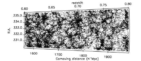
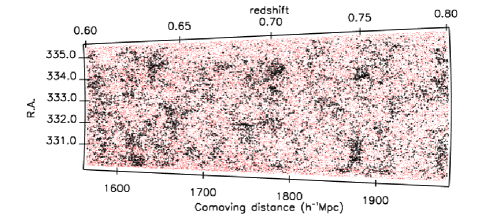
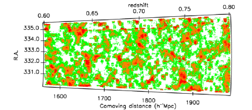
Figure 2: 2D distribution of galaxies (where the projected $Dec$ covers a range of $1.5^{\circ}$) in one of the W4 field mock catalogues used in this work. Top: all galaxies in the reference mock catalogue (100% sampling rate, the redshift includes cosmological redshift and peculiar velocity). Middle: galaxies in the Test D mock catalogue (see Sect. 4.1 for more details). The catalogue includes $\sim 35$% of galaxies in quadrants (black points) with spectroscopic redshift, while the remaining 65% in quadrants and all the galaxies in gaps have a photometric redshift (red dots). Bottom: Equal probability contours for the ZADE probability function $P(z_{i})$ (see Sect. 3.1 for details). Colour code is set according to the statistical weight $w_{ZADE}$. Red: $w_{ZADE}\geq 0.2$, Orange: $0.1\leq w_{ZADE}<0.2$. Green: $0.05\leq w_{ZADE}<0.1$.

3.2 Cloning

This method replicates the spatial position of spectroscopic galaxies near the edges of the surveyed areas into the unobserved regions (gaps and missing quadrants) to preserve the coherence of the large-scale structure without necessarily reconstructing the actual position of the missing objects.

We proceed as follows. A spectroscopic galaxy in a quadrant with 3D coordinates $ra_{0}$, $dec_{0}$ and $z_{0}$ (where $z_{0}$ is the spectroscopic redshift) is cloned in a gap with new coordinates $ra_{g}$,  $dec_{g}$,  $z_{g}$ assigned in two steps:

- STEP 1. We define $z_{g}$ = $z_{0}$ plus an error extracted from a Gaussian distribution with $\sigma$=0.0005(1+$z_{0}$), i.e. the typical spectroscopic redshift error; $ra_{g}$ and $dec_{g}$ are cloned from $ra_{0}$ and $dec_{0}$, by adding or subtracting an angular offset to either the $ra_{0}$ or $dec_{0}$ equal to the angular distance between the real galaxy and the edge of gap multiplied by two.

- STEP 2. Once $ra_{g}$, $dec_{g}$, and $z_{g}$ are assigned according to STEP 1, $ra_{g}$ and $dec_{g}$ are set equal to $RA$ and $Dec$ of the closest photometric galaxy in the gaps. We compute an adimensional distance between the position of the cloned galaxy ($ra_{g}$,  $dec_{g}$,  $z_{g}$) and the position of the photometric galaxies ($ra_{p}$,  $dec_{p}$,  $z_{p}$) using the formula

$$dist^{2}=\frac{(z_{g}-z_{p})^{2}}{\Delta_{z}^{2}}+\alpha\frac{(ra_{g}-ra_{p})^{2}+(dec_{g}-dec_{p})^{2}}{\Delta_{ang}^{2}},$$ (1)

where $\Delta_{z}$ and $\Delta_{ang}$ are two normalisations, namely $\Delta_{z}=0.035(1+z_{g})$ (i.e. the photometric redshift error) and $\Delta_{ang}=1$ arcmin; $RA$ and $Dec$ are expressed in arcmin; $\alpha$ is an ad-hoc chosen factor used to transform angular distances into redshift distances. A photometric galaxy can only be assigned to one single cloned galaxy.

Like ZADE, we also used the cloning method to fill single missing quadrants. The result of cloning applied to the VIPERS field W4 is shown in Fig. 3. In principle, we could also fill regions bigger than a quadrant (i.e. missing pointings), but in this way galaxies would be cloned from more and more distant regions, not preserving the large-scale coherence of galaxy clustering on the scales of interest.

We did not attempt to use cloning to correct for a low sampling rate. We find some studies that used cloning to correct small-scale incompleteness due to fibre collisions (see e.g. Blanton et al. 2005; Lavaux & Hudson 2011). Given the way we implemented the cloning (i.e., moving the cloned galaxy to the $RA-Dec$ position of a real photometric galaxy), its use on all scales to correct for sampling rate would simply result in retaining all the photometric galaxies in the new catalogue, and move their $z_{p}$ to the $z_{s}$ of the closest spectroscopic galaxy. This is very similar to implementing ZADE and retaining only the highest peak (with weight equal to 1) of the $z$ distribution obtained by multiplying the $z_{p}$ PDF by $n(z_{s})$. We tested this ZADE configuration (see the previous section), and we found that it does not perform as well as full ZADE in recovering the counts in cells.

Figure 3: Top: the real $RA-Dec$ distribution of VIPERS spectroscopic galaxies in the W4 field. Bottom: as in the top panel, but now gaps are filled with cloned galaxies.

The cloning method allows us to fill the gaps with a sampling rate similar to the one in the nearby cloned areas. On such a galaxy sample, it is possible to apply a non-parametric method to compute the 3D local density. As an example, we applied a 3D Voronoi-Delaunay tessellation to the cloned real VIPERS samples. The Voronoi diagram (Voronoi 1908) consists in a partition of 3D space in polyhedra, where each polyhedron encloses a galaxy and defines the unique volume containing all the points that are closer to that galaxy than to any other in the sample. The Delaunay complex (Delaunay 1934) defines the tetrahedra whose vertices are galaxies that have the property that the unique sphere that circumscribes them does not contain any other galaxy. The centre of the sphere is a vertex of a Voronoi polyhedron, and each face of a Voronoi polyhedron is the bisector plane of one of the segments that link galaxies according to the Delaunay complex.

A 3D Voronoi-Delaunay tessellation has already been used successfully for cluster identification in optical spectroscopic surveys (Marinoni et al. 2002; Gerke et al. 2005; Knobel et al. 2009; Cucciati et al. 2010), its power residing in exploiting the natural clustering of galaxies without any scale length chosen a priori. We applied a 3D Voronoi-Delaunay tessellation to the cloned PDR-1, and we used the inverse of the Voronoi volumes as a proxy for local density. Figure  4 shows 3D maps of the isosurfaces enclosing the regions with measured densities in the highest and lowest tails of the density distribution (i.e. densities above or below given thresholds). One can see very clearly that the highest densities form filamentary structures, while lowest densities enclose more spherical regions. The study of the topology of such regions goes beyond the aim of this paper, but Fig. 4 illustrates the potential of using a large and deep spectroscopic survey without gaps and roughly homogeneous coverage.

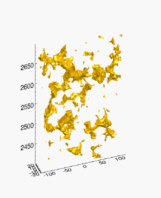
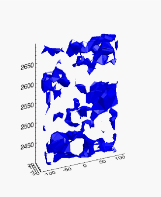
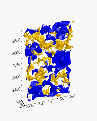
Figure 4: The 3D VIPERS density field obtained by filling gaps with the cloning method and computing the density within Voronoi volumes. Left: the isosurface enclosing the highest densities. Centre: the isosurface enclosing the lowest densities. Right: the isosurfaces of lowest and highest densities overplotted. One can see clearly that the highest densities form filamentary structures, while the lowest densities enclose more spherical regions. The plot shows the W1 field with RA$<$35.3 deg to avoid the missing pointing at RA$\sim 35.5$. Axes are in comoving coordinates (expressed in $\,h^{-1}{\rm Mpc}$): $x$ and $y$ are arbitrarily centred on the $RA-Dec$ centre of the considered field, and the $z$-axis corresponds to the redshift range $0.65\lesssim z\lesssim 0.75$.

3.3 Wiener filter

The Wiener filter differs from the previous methods in that it aims at reconstructing the continuous density field rather than the position of specific galaxies. It is a Bayesian method based upon statistical assumptions on the density field, namely that both the distribution of the over-density field $p(\delta)$ and the likelihood of observing $N$ galaxies given $\delta$, $p(N|\delta)$, are Gaussian distributions. The filter may be derived by maximising the posterior distribution given by Bayes formula:

$$p(\delta|N)=p(N|\delta)p(\delta)/p(N).$$ (2)

Although the prior and likelihood are modelled as Gaussian, the resulting estimated density field may be strongly non-Gaussian according to the constraints given by the observations.

To estimate the continuous density field, we bin the survey volume with cubic cells with size $2\,h^{-1}{\rm Mpc}$. Galaxies are assigned to the nearest cell. For a survey sub-volume indexed by $i$, the expected galaxy count is modelled as

$$\langle n_{i}\rangle=w_{i}\bar{n}(1+\delta_{i}),$$ (3)

where $w_{i}$ is the selection function and $\bar{n}$ the mean number of galaxies per cell. The selection function is determined by the product of the TSR, SSR, and CSR and also accounts for the angular geometry of the survey. The mean density $\bar{n}$ may be inferred from the observations by

$$\bar{n}=\frac{\sum_{i}n_{i}}{\sum_{i}w_{i}},$$ (4)

while the observed galaxy over-density, weighted by the selection function, is

$$\delta_{obs,i}\equiv w_{i}\delta_{i}=\frac{n_{i}}{\bar{n}}-w_{i}.$$ (5)

The Wiener filter depends on the covariance between cells given by a model correlation function, $S_{ij}\equiv\langle\delta_{i}\delta_{j}\rangle$, which we write in matrix notation. The computation is carried out in Fourier space and so, rather than the correlation function, we use the power spectrum computed with CAMB (Lewis et al. 2000; Takahashi et al. 2012) for the fiducial cosmology. We also express the selection function (in configuration space) as a diagonal matrix $W_{ii}=w_{i}$. Following the derivation by Kitaura et al. (2009, 2010), we may find the Wiener estimate for the over-density $\hat{\delta}$ by solving

$$\sum_{j}\left(\left[\mathsf{S}^{-1}\right]_{ij}+W_{ij}\bar{n}\right)\hat{\delta_{j}}=\bar{n}\delta_{obs,i}.$$ (6)

To solve this equation we use the iterative linear conjugate gradient solver included in the scientific python library SciPy. From now on, we refer to this method simply as ‘WF’.

3.4 Poisson-Lognormal Filter

We further investigate Bayesian estimation methods by adopting a lognormal form for $p(\delta)$. The lognormal distribution gives a more accurate description of the density field particularly in low and high-density environments (Coles & Jones 1991). We take a Poisson model for the likelihood $p(N|\delta)$. Following Kitaura et al. (2010), we define $s$ as the logarithmic transform of the over-density, ${\bf s}\equiv\ln(1+\delta)$.

Empirical tests show that the power spectrum of ${\bf s}$, $P_{\ln(1+\delta)}(k)$, follows the shape of the linear power spectrum: $P_{\ln(1+\delta)}(k)\approx aP_{linear}(k)$ (Neyrinck et al. 2009). The amplitude $a$ depends on the higher order moments of the field $\delta$ and is sensitive to the adopted smoothing scale. In the present analysis, we define the density over a grid with resolution $2\,h^{-1}{\rm Mpc}$ and set $a=0.2$ on the basis of numerical tests. Expressing the covariance in Fourier space, we take (in redshift space) $S_{L,ii}=aP_{linear}(k_{i})$.

Following the Gaussian case discussed above, we may derive the following equation that may be solved for $\hat{\delta}$ (Kitaura et al. 2010)

$$n_{i}-w_{i}\bar{n}(1+\hat{\delta}_{i})-\sum_{j}\left[\mathsf{S}_{L}^{-1}\right]_{ij}\left(\ln(1+\hat{\delta}_{j})-\lambda_{j}\right)-1=0.$$ (7)

We solve Eq. 7 for $\hat{\delta}$ with a nonlinear conjugate gradient solver using a Newton-Raphson solver with a Polak-Ribiere step. From now on, we refer to this method simply as ‘LNP’.

4 Counts-in-cells reconstruction

The aim of this paper is to find the best way to fill the gaps between quadrants and the areas where there are missing quadrants, in presence of all observational biases listed in Sect. 2.3. To gauge the success of a filling method we assess its ability to reconstruct the counts on a cell-by-cell basis and to separate high- from low-density regions from the probability distribution of the counts.

In Sect. 4.1 we list the mock galaxy catalogues used to study the effects of the different VIPERS observational biases to counts in cells. In Sect. 4.2 we describe the redshift bins and samples used in the analysis. In Sect. 4.3 we describe the tests carried out to estimate the robustness of the counts in cells given the biases.

4.1 Test levels

To estimate the contribution of each observational bias to the total error in counts in cells reconstruction, we mimic their effect separately in the mocks. Each source of error is investigated by means of a specific ‘test’.

For each light cone, our reference catalogue is the parent photometric mock catalogue (see Sect. 2.2), which has flux limit $i_{AB}=22.5$ and 100% sampling rate. We work in redshift space, so galaxies in these mocks have redshifts obtained combining cosmological redshift and peculiar velocities.

All mock catalogues used to assess the impact of the individual sources of error are drawn from the reference catalogue, and are called ‘test catalogues’. They are listed below, specifying the source of error they were designed to include.

Test A: The impact of the spectroscopic redshift error. We mimic this effect by adding the VIPERS spectroscopic redshift error to the reference catalogues. We do this by adding to the redshift $z_{i}$ of each galaxy a random value extracted from a Gaussian with $\sigma=0.0005(1+z_{i})$. In these mocks there are no gaps, and the sampling rate is 100%.

Test B: The impact of the performances of the gap-filling method. We use mock catalogues obtained from the reference catalogue, by removing galaxies in gaps and missing quadrants. Sampling rate and redshift of the galaxies falling in observed quadrants are unaltered. Since some of the methods used to fill the gaps (ZADE and cloning) make use of the photometric redshift of the galaxies falling in the gaps, we actually re-insert such galaxies into the catalogues, when needed, but we added to their redshift a photometric redshift error. We do this by adding to the redshift $z_{i}$ of each galaxy a random value extracted from a Gaussian with $\sigma=0.035(1+z_{i})$.

Test C1: The impact of a low sampling rate. We use mock catalogues obtained from the reference catalogue by removing randomly 65% of the galaxies to reach an overall sampling rate of 35% as in VIPERS. In these mocks there are no gaps, and the redshift of the retained galaxies is unaltered. As in Test B, we re-inserted the unretained galaxies mimicking for them a photometric redshift error, because the ZADE method uses them to correct for the sampling rate.

Test C2: The impact of low and inhomogeneous sampling rate. Here we want to test not only an average sampling rate of 35%, but also its modulation quadrant by quadrant, as given by the tool SPOC, used to choose VIPERS targets (see Sect. 2.1). We build the required mock catalogue as follows. First we apply SPOC to the reference catalogue, obtaining a catalogue with gaps and a sampling rate varying quadrant by quadrant. This is likely to mimic the VIPERS TSR, which is $\sim 40$%, so we further depopulate this catalogue randomly to reach an average sampling rate of 35% (to account for the SSR). This way we have a VIPERS-like catalogue (varying sampling rate and empty gaps). Since we do not want to test the effects of gaps in this test, we add the galaxies again in the gaps, with a homogeneous sampling rate of 35%, so at the end in these mock catalogues there are no gaps, and the redshift of the retained galaxies (also the 35% in gaps) is unaltered with respect to the reference catalogue. Again, the remaining $\sim 65$% of galaxies have been assigned a photometric redshift error to make them available if needed (see the ZADE method).

Test D: The impact of all of the above effects together, i.e. using VIPERS-like mock catalogues. These catalogues have been prepared as in Test C2, with the exceptions that i) galaxies retained in quadrants ($\sim 35$%) have a spectroscopic redshift error as in Test A, and ii) all of the other galaxies (100% of galaxies in gaps or in missing quadrants, and the remaining $\sim 65$% in quadrants) have a photometric redshift error.

4.2 Galaxy samples

VIPERS covers a wide redshift range and, because of its flux-limited selection, the survey samples only the more luminous galaxies at higher redshift. As a result, the mean number density of objects decreases at higher redshift. In this work, we want to use samples with a constant number density as a function of redshift, to ease the interpretation of our results and to better compare them with similar choices in the literature. We have divided the redshift range in three shells and applied a luminosity cut (in $B$-band absolute magnitude $M_{B}$) to obtain a set of volume-limited, luminosity complete subsamples, with constant number density in the given redshift bin. The three samples adopted in this work are

1. - $0.5<z<0.7$, with cut at $M_{B}-5\log_{10}(h)=-18.9-z$,

2. - $0.7<z<0.9$, with cut at $M_{B}-5\log_{10}(h)=-19.4-z$,

3. - $0.9<z<1.1$, with cut at $M_{B}-5\log_{10}(h)=-19.9-z$,

where the redshift dependence of the luminosity thresholds is designed to account for evolutionary effects, since it roughly follows the same dependence on redshift as the $M^{*}$ of the galaxy luminosity function (see e.g. Kovač et al. 2010). In the reference mock catalogues, i.e. those with flux limit $i_{AB}=22.5$ and 100% sampling rate, the galaxy number densities (averaged over all the mock catalogues) in the three samples are $1.1\times 10^{-2}$, $4.3\times 10^{-3}$, and $1.7\times 10^{-3}$ galaxies per $(\,h^{-1}{\rm Mpc})^{3}$. The variance of these values among the 26 catalogues is $\sim 10$% in the sample at lowest redshift and $\sim 5$% in the other two.

We show results only for the central redshift bin, to minimise the number of plots in the paper, but we will discuss the results obtained in all three redshift bins (see Sect. 5.1.2 and Fig. 6).

4.3 Counts-in-cells comparison

In each kind of mock catalogue, we perform counts in cells on spherical cells with radius $R=5$ and $8\,h^{-1}{\rm Mpc}$ comoving ($R_{5}$ and $R_{8}$ from now on), distributed randomly in the field. Galaxy over-densities are obtained by counts in cells as $\delta_{N}=N/\langle N\rangle-1$, where $N$ represents the number of objects in the cell, and $\langle N\rangle$ is the mean galaxy count in cell in each of the considered redshift bins.

Our first test, described in Sect. 5.1 consists of a cell-by-cell comparison of $\delta_{N}$ in the reference mock catalogue ($\delta_{N}^{R}$) and in the different test catalogues ($\delta_{N}^{A}$, $\delta_{N}^{B}$, $\delta_{N}^{C1}$, $\delta_{N}^{C2}$, $\delta_{N}^{D}$). The results of this comparison are described in Sect. 5.1. This is indeed a very demanding test. More demanding than, for example, the recovery of the one-point probability of galaxy counts, $P(N)$. This latter issue will be addressed in detail elsewhere in the more general framework of the recovery of the probability distribution function of the underlying galaxy density field (Bel et al. in prep.) and of the galaxy bias (Di Porto et al. in prep.). Here we also consider the $P(N)$ of the reconstructed counts, but we use it only as a tool to separate high- from low- density regions. Assessing the ability to effectively separate these environments is the goal of our second test.

Our second test, explained in Sect. 5.2 aims at finding which gaps-filling method allows us to best disentangle the lowest and highest $\delta_{N}^{R}$ when selecting the extremes of the $P(\delta_{N}^{D})$ distribution.

We note that the WF and LNP methods give an estimate of the density field on a grid, and so the counts in cells measurement cannot be made in the same way as for the ZADE and cloning methods. To make the comparison, we compute $\delta$ in a given spherical cell by averaging the enclosed grid cell values.

5 Results

5.1 Density-density comparison

The results of Tests A, B, C1, and C2 are extensively presented in Appendix A. In this section we summarise them, and discuss Test D in detail, which includes all the sources of uncertainty of the other tests.

The plots of Figures 10,  11, 12, 13, and 5 show the comparison between the density contrast in the reference catalogue ($\delta_{N}^{R}$, on the x-axis) and in the test catalogues ($\delta_{N}^{A}$, $\delta_{N}^{B}$, $\delta_{N}^{C1}$, $\delta_{N}^{C2}$, $\delta_{N}^{D}$, on the y-axis). A quantitative comparison of all the tests shown in these figures is reported in Table 1. The reference catalogue has a 100% sampling rate down to $i$=22.5, and no gaps. Test catalogues are listed in Sect. 4.1 and are different in each set of plots.

We notice that, for $\delta\rightarrow-1$, the lines in the top panels tend to diverge because of the logarithmic scale of the axes (which emphasises the low- and intermediate-density regimes). Moreover, for $\delta\rightarrow-1$, the denominator of the normalised residuals (the variable in $y$-axis in the bottom panels) approaches zero and residuals rapidly increase. This is an artefact related to our definition of residuals.

The results of Tests A, B, C1, and C2 can be summarised as follows.

Test A. The effects of the spectroscopic redshift error on the counts in cell is to induce a small systematic underestimate at high densities (for $1+\delta^{R}_{N}\gtrsim 5$). For both radii, the systematic error is comparable to the scatter for intermediate or high densities. Applying the WF or LNP method to recover the counts in the reference catalogue does not improve the reconstruction.

Test B. For all methods the scatter is larger than found in Test A, while the systematic error is comparable. The ZADE method shows the smallest scatter with low systematic error for both cases $R_{5}$ and $R_{8}$. The accuracy of the reconstruction is better for $R_{8}$ than $R_{5}$.

Test C1 and C2. In Test C1, for all three methods, and for both $R_{5}$ and $R_{8}$, the scatter is larger or comparable to the systematic error, with possibly the exception of the highest densities. Moreover, the systematic error and the scatter due to low sampling rate are always greater than those due to gaps, and much more than those due to the spectroscopic redshift error. The results for Test C2 are only slightly worse than those of Test C1.

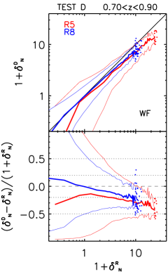
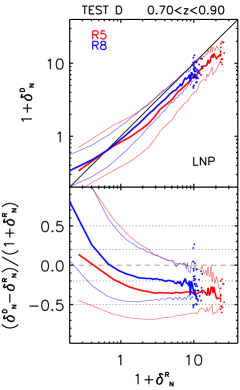
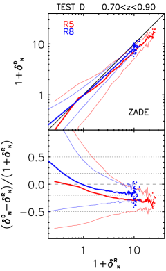
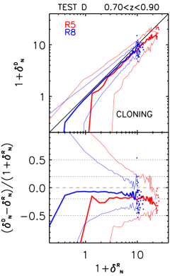
Figure 5: Comparison of overdensities for Test D, for WF, LNP, ZADE, and cloning (from left to right), for the redshift bin $0.7<z<0.9$ and tracers with $M_{B}-\log_{10}(h)\leq-19.4-z$. x-axis: overdensity in the reference catalogue ($1+\delta^{R}_{N}$); y-axis, top panels: overdensity in the test catalogue ($1+\delta^{B}_{N}$); y-axis, bottom panels: relative error ($(\delta^{B}_{N}-\delta^{R}_{N})/(1+\delta^{R}_{N})$). The thick lines are the median value of the quantity displayed on the y-axis in each given x-axis bin. Thin lines represent the 16th and 84th percentiles of its distribution. Points are single cells, when cells per bin are $<20$ (in which case we do not compute a median and percentiles). Red and blue lines/symbols are for spheres with radius $R_{5}$ and $R_{8}$, respectively. See text for details about tests.

5.1.1 Test D

In Test D we combine all of the sources of uncertainty of the previous tests (spectroscopic redshift errors, gaps, low and not homogeneous sampling rate), thus using mock catalogues that mimic all the VIPERS characteristics. Results are shown in Fig. 5.

We did not use the cloning method to correct for the sampling rate (see Sect. 3.2), but in Test D we need to account for it. After applying the cloning, we are left with a sample of original and copied galaxies with no gaps, but with a sampling rate varying quadrant by quadrant. To correct for this, we weighted each galaxy by the inverse of the relevant sampling rate.

In contrast, ZADE can be used not only for filling the gaps, but also to correct for the sampling rate in quadrants (see Sect. 3.1). Alternatively, we can use ZADE to fill the gaps, but treat the low sampling rate by weighting spectroscopic galaxies in quadrants by the inverse of the sampling rate. We verified that this second method gives a poorer reconstruction of counts in cells than the one based solely on ZADE (in particular, it gives a random error 15-20% larger), so here we only show the results with ZADE correcting for both gaps and sampling rate.

Figure  5 shows the cumulative effects of all sources of uncertainties considered in the previous tests:

• A general underestimate of the counts, at all densities, with the exception of LNP and ZADE over-predicting counts in the very underdense regions.

• At high overdensities the random errors are smaller than or comparable to the systematic ones in all cases except for the cloning method, meaning that systematic errors are indeed significant.

• The method less affected by systematic errors is cloning. This is evident in the high-density tail. This, however, is also the method affected by the largest random errors. Random errors are the smallest when the ZADE method is applied.

Table 1 shows a more quantitative comparison between $\delta_{N}^{R}$ and $\delta_{N}^{D}$. We list in the table the values of the slope and of the intercept of the linear fit performed on the thick lines in the top panels of Fig. 5. Errors on $\delta_{N}^{D}$ are set equal to the width of the probability of $\delta_{N}^{D}$ given $\delta_{N}^{R}$, $P(\delta_{N}^{D}|\delta_{N}^{R})$ measured at the $16^{th}$ and $84^{th}$ percentiles. The table also shows the linear correlation coefficient $r$ and the Spearman coefficient $\rho$, for the same set of $x$ and $y$ values used for the linear fit. While $r$ tells us how well the two variable are linearly correlated, $\rho$ returns the degree of correlation (not necessarily linear) between $x$ and $y$. This second test is also important for our analysis: even if $\delta_{N}^{D}$ is not linearly correlated with $\delta_{N}^{R}$, if $\rho$ is close to 1 the two variable can be linked with a monotonic function, allowing us to disentangle low and high densities (see Sect. 5.2). The table shows that both $r$ and $\rho$ are always very close to unity.

We obtain a lower Spearman coefficient when we compute it on the values of $1+\delta_{N}^{R}$ and $1+\delta_{N}^{D}$ of the single cells instead of their median value in each density bin. This is shown in the table as $\rho_{cells}$. This result is due to the fact that the probability of galaxy overdensity $P(\delta_{N})$ is skewed towards low densities (see Fig. 7 discussed later on): on a cell-by-cell basis, low densities weight more and, given that the random error at low densities is larger, the correlation between $\delta_{N}^{R}$ and $\delta_{N}^{D}$ is weaker if we use single cells instead of median values in equally spaced bins of $\delta_{N}^{R}$. Nevertheless, both $\rho$ and $\rho_{cells}$ are significatively different from zero, since the significance of the Spearman coefficient depends also on the number of used points. In our case, the number of spheres is so large that $\rho_{cells}$ results more significantly different from zero than $\rho$.

5.1.2 Redshift dependence

The results of Test D in the lower ($0.5<z<0.7$) and higher ($0.9<z<1.1$) redshift bins are quite similar to those presented in Fig. 5. The evolution with redshift of the systematic and random error in test D for the four methods is shown in Fig. 6. The figure refers to a given overdensity value ($1+\delta^{R}_{N}=5$), but trends with redshift are qualitatively similar for other $\delta^{R}_{N}$ (the absolute value might be different).

For $R_{5}$, the systematic error for ZADE does not evolve significantly with redshift, while its random error is 5-10% smaller and 5-10% larger at $0.5<z<0.7$ and $0.9<z<1.1$, respectively, with respect to the central redshift bin. For the WF and LNP methods the systematic error increases with redshift, but the random error does not evolve significantly. For the cloning method, both random and systematic errors increase with redshift. For $R_{8}$, all the trends visible for $R_{5}$ are much milder. These results also hold for a intermediate test level (e.g., Tests B and C).

We note that we use different luminosity thresholds in each redshift bin, so we also verified that our results do not change significantly when keeping the same luminosity threshold and moving to lower redshift. This means that the different levels of random and systematic errors found at different redshifts are mainly due to the different density of the used tracers and not to the evolution with redshift of the typical density of a given set of tracers.

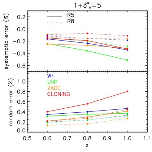
Figure 6: Systematic (top) and random (bottom) relative errors in the reconstruction of $\delta^{R}_{N}$ in Test D, in the 3 redshift bins considered in this study ($x-$axis). We only show results for $\delta^{R}_{N}+1=5$, but trends with redshift are similar for other values. These values correspond, respectively, to the thick and thin lines in the bottom panels of Fig. 5, for the given $\delta^{R}_{N}$ value. The value of the scatter is obtained by averaging the lower and upper values of the scatter (the two thin lines in Fig. 5). Solid line is for $R_{5}$ and dotted line for $R_{8}$. Different colours correspond to the different methods (blue: WF; green: LNP; orange: ZADE; red: cloning).

Table 1: Linear fit of the median values in the scatter plots (top panels) of Figures 10, 11, 12, 13, and 5. For the fit we use $x=1+\delta^{R}_{N}$ (central value of each $1+\delta^{R}_{N}$ bin) and $y=median(1+\delta^{T}_{N})$, i.e. the value of the thick line in the plots in the given $1+\delta^{R}_{N}$ bin. Errors of $\delta^{T}_{N}$ are measured at the $16^{th}$ and $84^{th}$ percentiles of the conditional probability function $P(\delta_{N}^{T}|\delta_{N}^{R})$ (thin lines in the above-mentioned figures). The table shows the intercept and slope of the linear fit, the linear correlation coefficient (r), the Spearman coefficient ($\rho$). The columns “$\rho_{cells}$” show the Spearman coefficient obtained using the density in each single cell instead of the median density value per bin.

Method	$R=5\,h^{-1}{\rm Mpc}$					$R=8\,h^{-1}{\rm Mpc}$
	Intercept	Slope	$r$	$\rho$	$\rho_{cells}$	Intercept	Slope	$r$	$\rho$	$\rho_{cells}$
TEST A
WF	-0.03$\pm$ 0.16	0.87$\pm$ 0.02	0.999	0.999	0.889	0.04$\pm$ 0.07	0.93$\pm$ 0.02	0.999	1.000	0.972
LNP	-0.07$\pm$ 0.16	0.95$\pm$ 0.02	0.999	1.000	0.866	0.05$\pm$ 0.07	1.00$\pm$ 0.02	0.999	0.999	0.964
Counts	-0.04$\pm$ 0.15	0.92$\pm$ 0.02	0.999	0.999	0.907	0.02$\pm$ 0.06	0.96$\pm$ 0.01	0.999	1.000	0.974
Test B
WF	$-0.06\pm 0.19$	$0.92\pm 0.03$	0.998	0.997	0.868	$-0.00\pm 0.09$	$0.98\pm 0.03$	0.999	0.999	0.951
LNP	$-0.03\pm 0.17$	$0.95\pm 0.03$	0.998	0.998	0.853	$0.03\pm 0.08$	$1.02\pm 0.03$	0.999	0.999	0.948
ZADE	$0.03\pm 0.16$	$0.94\pm 0.02$	0.998	0.999	0.909	$0.02\pm 0.07$	$0.97\pm 0.02$	0.999	1.000	0.970
Cloning	$-0.06\pm 0.17$	$0.93\pm 0.03$	0.998	0.999	0.894	$-0.02\pm 0.08$	$0.98\pm 0.03$	0.999	0.999	0.945
TEST C1
WF	-0.16$\pm$ 0.21	0.89$\pm$ 0.04	0.997	0.993	0.763	-0.02$\pm$ 0.12	0.95$\pm$ 0.03	0.999	0.999	0.896
LNP	-0.04$\pm$ 0.19	0.86$\pm$ 0.04	0.995	0.993	0.766	0.06$\pm$ 0.09	0.92$\pm$ 0.03	0.998	0.999	0.896
ZADE	0.00$\pm$ 0.22	0.83$\pm$ 0.03	0.998	0.997	0.808	0.03$\pm$ 0.10	0.93$\pm$ 0.03	0.999	1.000	0.921
Test C2
WF	$-0.06\pm 0.22$	$0.81\pm 0.04$	0.997	0.996	0.765	$0.04\pm 0.12$	$0.88\pm 0.04$	0.998	0.997	0.896
LNP	$0.04\pm 0.19$	$0.78\pm 0.04$	0.997	0.995	0.768	$0.12\pm 0.10$	$0.84\pm 0.04$	0.999	0.997	0.895
ZADE	$0.09\pm 0.23$	$0.78\pm 0.03$	0.998	0.999	0.811	$0.08\pm 0.10$	$0.88\pm 0.03$	0.999	0.998	0.922
Test D
WF	$0.08\pm 0.27$	$0.66\pm 0.04$	0.993	0.994	0.685	$0.09\pm 0.15$	$0.81\pm 0.05$	0.995	0.992	0.837
LNP	$0.17\pm 0.21$	$0.63\pm 0.04$	0.996	0.994	0.698	$0.18\pm 0.11$	$0.74\pm 0.05$	0.997	0.992	0.844
ZADE	$0.25\pm 0.26$	$0.65\pm 0.03$	0.996	0.998	0.730	$0.12\pm 0.13$	$0.82\pm 0.04$	0.999	0.998	0.873
Cloning	$-0.20\pm 0.01$	$0.76\pm 0.05$	0.995	0.992	0.650	$-0.07\pm 0.14$	$0.90\pm 0.05$	0.997	0.996	0.799

5.2 Distinguishing between low- and high- density environments

In this section we study how well we can disentangle low and high densities in the reference catalogue using the reconstructed counts in Test D. Although the recovery of $P(\delta_{N})$ is not the main goal of the paper, but just an intermediate step to separate high-from low-density environments, it is interesting to compare the $P(\delta_{N}^{D})$ reconstructed with the various methods to the one obtained from the reference mock catalogues $P(\delta_{N}^{R})$. We make this comparison in Fig. 7, in which we show the different probabilities of counts multiplied by $(1+\delta_{N})$ to emphasise differences in the low- and high-count tails of the distribution.

The figure shows that all methods recover the reference $P(\delta_{N})$ at $\sim 1-2\sigma$ level, with the largest differences being at the lowest densities. We remind the reader that the WF and LNP methods produce filtered counts, while the counts in our reference catalogue are not filtered. We further verified that, as expected, the WF and LNP are in better agreement with the reference $P(\delta_{N}^{R})$ when the comparison is made using densities obtained from smoothed counts also in the reference catalogue.

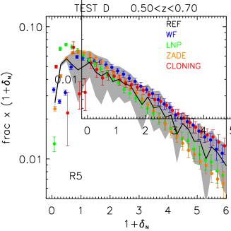
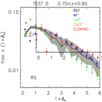
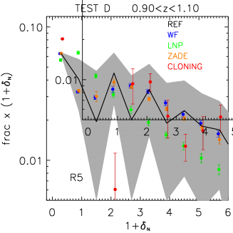
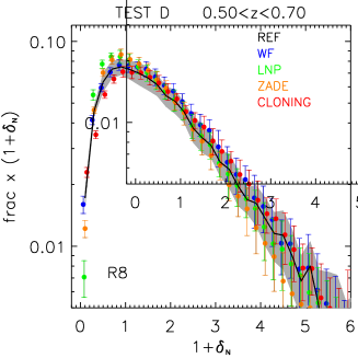
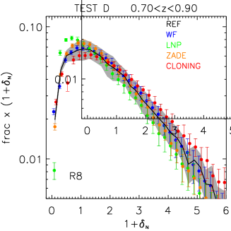
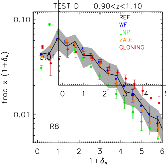
Figure 7: Distributions of the reference (black line) and Test D overdensities (lines) for the three redshift bins $0.5<z<0.7$, $0.7<z<0.9$, and $0.9<z<1.1$ (from left to right), with tracers with $M_{B}-\log_{10}(h)\leq-18.9-z$, $M_{B}-\log_{10}(h)\leq-19.4-z$, and $M_{B}-\log_{10}(h)\leq-19.9-z$, respectively. Top row is for cells with $R=5\,h^{-1}{\rm Mpc}$, bottom row for cells with $R=8\,h^{-1}{\rm Mpc}$. Different colours are for different methods, as specified in the label: WF (blue), LNP (green), ZADE (orange), cloning (red). Grey-shaded area is the $rms$ around the black line, computed using the 26 light cones. To better appreciate the differences among the series of points, the $1+\delta_{N}$ distribution on the $y-$axis has been multiplied by the corresponding value of $1+\delta_{N}$ itself.

To disentangle low and high densities, we take the spheres with $\delta_{N}^{D}$ falling in the first and those falling in the fifth quintile of $P(\delta_{N}^{D})$, and we plot the corresponding $P(\delta_{N}^{R})$ for the selected spheres. As a reference, we do the same also for the third quintile of $P(\delta_{N}^{D})$. This way we can verify whether, considering very different environments in the reconstructed counts in cells, we are also sampling very different environments in the reference catalogue.

Results are shown in Fig. 8. The main result is that, in all cases, the first and fifth quintiles are separated well, for both $R_{5}$ and $R_{8}$. ZADE, LNP (not shown), and WF (not shown) give very similar results. This is because none of the methods outperforms the others, as also seen in Fig. 5. Table 2 lists the average values of the 16%, 50%, and 84% of all the distributions shown in Fig. 8. The average is done on the 26 mock catalogues. These results hold also for the lower and higher redshift bins. The table shows that the first and fifth quintile are always separated at least at $2\sigma$ level.

The intermediate densities (third quintile) are fully separated at $2\sigma$ level from the highest densities ($5^{th}$ quintile) in almost all the cases listed in Table 2 (the exceptions being the highest redshift bin for $R_{5}$, and the intermediate redshift bin for $R_{5}$ but only for the LNP method). In contrast, it is harder to separate the densities in the first and third quartiles for $R_{5}$, irrespective of the redshift bin and of the method used. This is due to the skewness of the $P(\delta_{N})$ and the large relative error in the reconstruction of low densities. Even if the Test D reconstruction is good enough to maintain a good shape of the $P(\delta_{N})$ (see Fig. 7), the relative error at low densities is too large to properly distinguish, locally, between low and intermediate densities. For $R_{8}$, the lowest and intermediate densities are separated at $\sim 2\sigma$ level, at least for $z<0.9$.

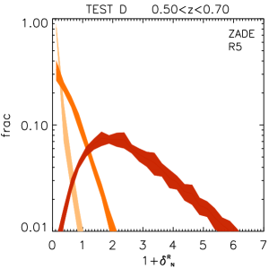
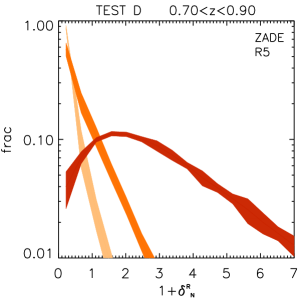
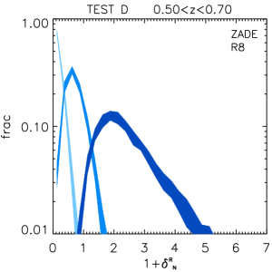
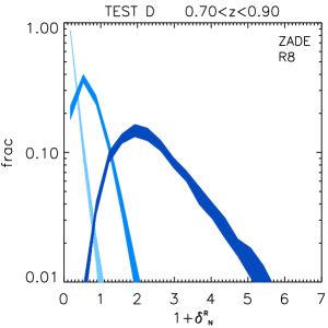
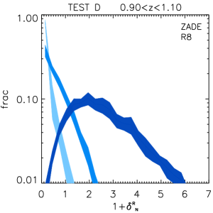
Figure 8: Distributions of reference overdensities for the spheres falling in the first, third and fifth quintiles of the density distribution computed in Test D, using ZADE. Left, middle and right panels are for the three redshift bins $0.5<z<0.7$, $0.7<z<0.9$ and $0.9<z<1.1$, with tracers with $M_{B}-\log_{10}(h)\leq-18.9-z$, $M_{B}-\log_{10}(h)\leq-19.4-z$ and $M_{B}-\log_{10}(h)\leq-19.9-z$, respectively. Shades of red (top) are for cells with $R=5\,h^{-1}{\rm Mpc}$, while shades of blue (bottom) for cells with $R=8\,h^{-1}{\rm Mpc}$. For both radii, colours from light to dark are for the first, third and fifth quintiles of the Test D density distribution. Bins on the x-axis are different in all panels (for smoothing purposes), so normalisation is not comparable among panels. All distributions are normalised to unity. Results obtained with the LNP method are very similar. See also Table 2.

Table 2: Values of the 16%, 50% and 84% of all the distributions of $(1+\delta_{N}^{R})$ shown in Fig. 8 (ZADE), and the corresponding values obtained with LNP. These values are given as mean values among all the used mock catalogues. Their typical $rms$ is of the order of 5-10% for $R_{5}$. For $R_{8}$, the typical $rms$ is of the order of 5-10% for the first and third quintiles, and of the order of 2-3% in the highest density quintile.

Redshift	Method	1st 20%			3rd 20%			5th 20%
		16%	50%	84%	16%	50%	84%	16%	50%	84%
$R=5\,h^{-1}{\rm Mpc}$
0.5$<$z$<$0.7	LNP	0.0	0.0	0.25	0.0	0.46	1.06	1.18	2.42	4.51
	ZADE	0.0	0.0	0.25	0.1	0.46	1.01	1.31	2.50	4.53
0.7$<$z$<$0.9	LNP	0.0	0.0	0.44	0.0	0.43	1.09	0.94	2.39	4.88
	ZADE	0.0	0.0	0.44	0.0	0.42	0.95	1.09	2.49	4.89
0.9$<$z$<$1.1	LNP	0.0	0.0	0.0	0.0	0.0	1.19	0.50	2.32	5.67
	ZADE	0.0	0.0	0.0	0.0	0.0	1.16	1.10	2.39	5.72
$R=8\,h^{-1}{\rm Mpc}$
0.5$<$z$<$0.7	LNP	0.0	0.14	0.34	0.38	0.66	1.05	1.44	2.20	3.50
	ZADE	0.0	0.14	0.31	0.41	0.67	1.01	1.54	2.24	3.53
0.7$<$z$<$0.9	LNP	0.0	0.11	0.35	0.30	0.62	1.12	1.36	2.25	3.57
	ZADE	0.0	0.10	0.32	0.32	0.62	1.07	1.47	2.29	3.61
0.9$<$z$<$1.1	LNP	0.0	0.0	0.37	0.01	0.52	1.19	1.18	2.31	4.10
	ZADE	0.0	0.0	0.30	0.13	0.52	1.11	1.30	2.37	4.14

5.3 Application to VIPERS

We computed the counts in cells in the two VIPERS fields, in the same spheres used for the mocks catalogues. Gaps and low sampling rate have been accounted for using the ZADE method. The spectroscopic sample that we used is the one described in Sect. 2.1. The photometric sample used to fill the gaps and reach 100% sampling rate in quadrants corresponds to the full photometric catalogue in the fields W1 and W4, complete down to $i_{AB}=22.5$ and from which we removed the galaxies included in our spectroscopic sample.

Figure  9 shows the probability of galaxy overdensity $P(1+\delta_{N})$ for the VIPERS sample (fields W1 and W4 altogether), compared with the $P(1+\delta_{N})$ in the reference mock catalogues and the one reconstructed in test D using ZADE. It is evident that the agreement between the VIPERS $P(1+\delta_{N})$, and the one reconstructed in VIPERS-like mocks is very good. For instance, the $20^{th}$, $50^{th}$, and $80^{th}$ percentiles of the $1+\delta$ distribution for $R_{5}$ and $0.7<z<0.9$ are 0.09, 0.55, and 1.65 for VIPERS, $0$, $0.44\pm 0.02$, $1.7\pm 0.1$ for the reference mock catalogue, and $0.08\pm 0.006$, $0.50\pm 0.01$, $1.66\pm 0.01$ for the VIPERS-like mock catalogues (Test D, reconstructed using ZADE). One can also notice that the real VIPERS density distribution at $0.7<z<0.9$ around the mean density ($1+\delta_{N}=1$) is higher than the one in the mock catalogues, but it is a very weak effect.

We note that this general agreement is not necessarily there by construction, since the HOD mock catalogues have been tuned to match the clustering properties (namely, the two point correlation function, see e.g. de la Torre et al. 2013 and Marulli et al. 2013) in VIPERS, and not the over-density distribution.

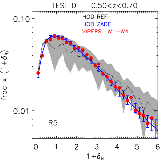
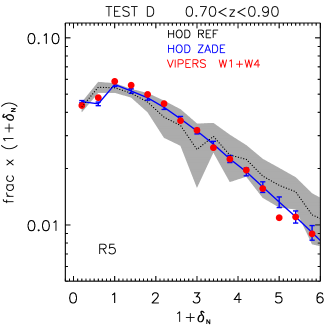
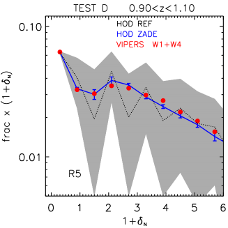
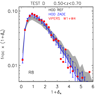
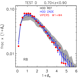
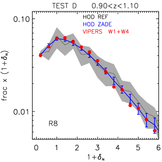
Figure 9: Distributions of reference (black line) and real VIPERS overdensities (points) for the three redshift bins $0.5<z<0.7$, $0.7<z<0.9$, and $0.9<z<1.1$ (from left to right), with tracers with $M_{B}-\log_{10}(h)\leq-18.9-z$, $M_{B}-\log_{10}(h)\leq-19.4-z$, and $M_{B}-\log_{10}(h)\leq-19.9-z$, respectively. Grey-shaded area is the $rms$ around the black line, computed using the 26 light cones. Top row is for cells with $R=5\,h^{-1}{\rm Mpc}$, bottom row for cells with $R=8\,h^{-1}{\rm Mpc}$. Real VIPERS overdensities are computed with the ZADE method. For comparison, the blue solid line with vertical error bars is the result of Test D (ZADE). To better appreciate the differences among the series of points, the $(1+\delta_{N})$ distribution on the $y-$axis has been multiplied by the corresponding value of $1+\delta_{N}$ itself.

6 Discussion and conclusions

The goal of this work has been to find the best way to fill empty areas in spectroscopic surveys so as to obtain the most reliable counts-in-cell reconstruction. As a test case, we study how to fill the gaps across VIMOS quadrants in the VIPERS survey. To tackle the problem, we applied four methods to fill the gaps and compared their performances using mock galaxy catalogues mimicking the sources of errors we want to correct for (not only gaps, but also sparse sampling and related systematic effects). For the first time we have performed a systematic comparison among gap-filling methods using different techniques that either directly use the observed, discrete galaxy distribution to fill the gaps or do this within the more general framework of reconstructing the underlying, continuous mass density field using suitable filtering techniques.

Our results can be summarised as follows:

1. On the scales we tested, the error budget is dominated by the sparseness of the sample.

2. All methods under-predict counts in high-density regions. This bias is in the range of 20-35%, depending on the cell size, method, and overdensity. This systematic bias is similar to random errors.

3. Random errors have similar amplitude for all methods, except cloning for which errors are significantly larger.

4. No method largely outperforms the others. LNP is certainly better than WF, and ZADE is to be preferred to cloning, but differences are not large, and methods with the smallest random errors (ZADE) can be more affected by systematic errors than others.

5. Random and systematic errors decrease with the increasing size of the cell, although in both cases considered ($R_{5}$ and $R_{8}$), systematic and random errors are of similar amplitude.

6. Recovering the correct overdensity in a generic resolution element is a more demanding test than reconstructing the correct one-point counts statistic. Our tests show that in a survey such as VIPERS the galaxy overdensity in a resolution element of 5 to $8\,h^{-1}{\rm Mpc}$ can be reconstructed with a typical error of about 25%, knowing that the estimate will be biased low by a similar amount.

7. With all methods, the first and fifth quintiles of the distribution of $(1+\delta_{N}^{D})$ correspond to well-separated regimes of the $(1+\delta_{N}^{R})$ distribution, at least at a $2\sigma$ level for both $R_{5}$ and $R_{8}$.

These results are quantitatively exact for VIPERS, because we tested the gap size and the sampling rate of this specific survey. Different values of gap size and/or sampling rate could produce a different result. Nevertheless, our results are of general interest for all surveys utilising a mosaic of non-contiguous fields.

Our results on the reconstruction of counts in cells are the basis to understand how well we can parameterise the galaxy local environment in a survey like VIPERS. The study of how environment affects galaxy properties is crucial to understanding galaxy evolution.

Clearly, for environmental studies, the counts in spherical cells distributed randomly in the field might not be the best choice, depending on the specific goal one wants to reach. For instance, other cell shapes can be preferred, such as cylindrical filters, that would allow us to take the ‘Fingers of God’ effect (Jackson 1972) into account in the highest densities. Moreover, the use of an adaptive scale (such as the distance from the $n^{th}$ nearest neighbour) could help reconstruct the highest densities. Thanks to mock galaxy catalogues embedded in DM simulations, it is also possible to compare the reconstructed density field to the underlying DM distribution. Such a comparison can give clues to how and why the local environment affects galaxy evolution (see e.g. Haas et al. 2012; Muldrew et al. 2012; Cucciati et al. 2012; Hirschmann et al. 2013). Building on the results we obtained in the present work, we will describe the parameterisation of local density in the VIPERS survey for environmental studies in a future work (Cucciati et al., in prep.)

We would like to point out that VIPERS has been designed to be a cosmological survey, but thanks to its observational strategy, the density of tracers is higher than other cosmological surveys at the same redshift (e.g. the WiggleZ survey, see Drinkwater et al. 2010). We have shown that this allows, for the first time, the reconstruction of environment on scales of $5\,h^{-1}{\rm Mpc}$ on a very large field at $0.5\lesssim z\lesssim 1.1$. This will have a strong impact in the characterisation of cosmic variance and rare populations (e.g. brightest galaxies) in environmental studies at this redshift. Moreover, the results obtained in this work with the ZADE method are also promising for environmental studies in future surveys such as EUCLID, which is based on a spectroscopic data set complemented by a photometric galaxy catalogue, with a photometric redshift error similar to the one in VIPERS.

Appendix A Results of the Tests A, B, C1 and C2

A.1 Test A

The goal of this test is to assess the impact of redshift measurement errors on the counts in cells. Results are shown in Fig. 10. The ZADE and cloning methods do not correct for spectroscopic redshift error, so for this test we only compare the WF and LNP methods.

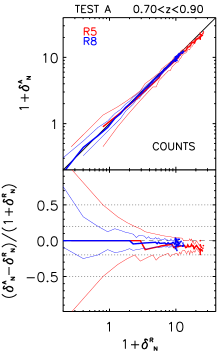
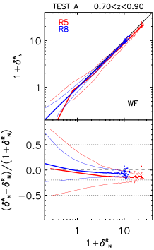
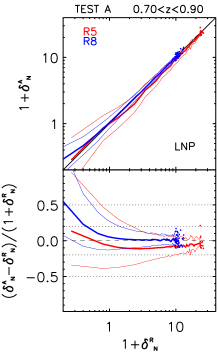
Figure 10: As in Fig. 5, but for Test A. ZADE and cloning are not used. $\delta^{A}_{N}$ in the left panel represents counts in cells in Test A without any attempt to correct for the spectroscopic redshift error (see text for details).

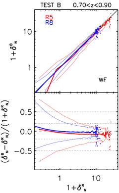
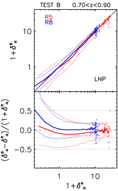
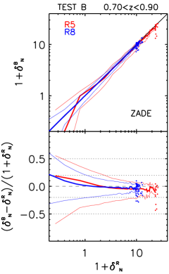
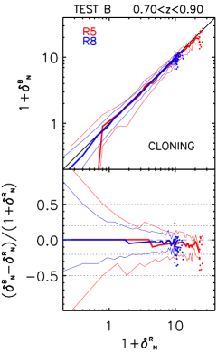
Figure 11: As in Fig. 5, but for Test B.

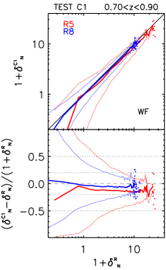
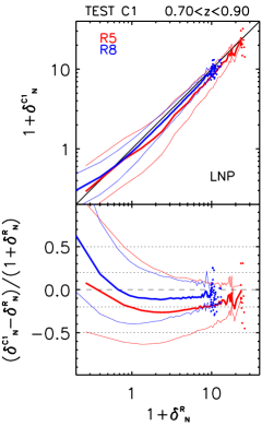
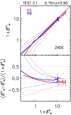
Figure 12: As in Fig. 5, but for Test C1. In this test the cloning method is not used (see text for details).

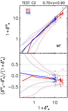
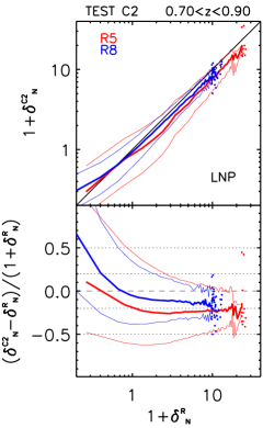
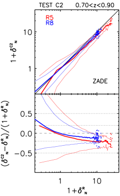
Figure 13: As in Fig. 5, but for Test C2. In this test the cloning method is not used (see text for details).

First, we verified the effects of the spectroscopic redshift error on the counts in cell when no attempt is made to correct for it (left panel in Fig. 10): this error does not induce systematic errors in regions of low/mean density (1+$\delta^{R}_{N}\leq 1$), while it systematically makes us underestimate the counts at high densities (by $\sim$8% for $R_{5}$ and $\sim$3% for $R_{8}$, for $1+\delta^{R}_{N}\gtrsim 5$). Random and systematic errors are significantly smaller for $R_{8}$ than for $R_{5}$, i.e. when the size of the cell is larger than the linear scale associated with the redshift error. For both radii, the systematic error is comparable to the scatter.

Applying the WF method to recover the counts in the reference catalogue does not improve the reconstruction, or even increases (almost double) the systematic error at high density for $R_{5}$. Applying the LNP method, the systematic error for $R_{5}$ slightly increases at high density (becoming $\sim 10$%), but disappears for $R_{8}$ (but at the expense of a larger random error, that approaches $\sim 10$%). Both estimates effectively smooth the density field, and thus the extremes of the density field are systematically underestimated, especially on smaller scales. For the WF method, the systematic error is comparable to the scatter, while for the LNP it is $\sim 50$% smaller, for both $R_{5}$ and $R_{8}$.

Even though our aim is to reconstruct counts in redshift space, we also compared the counts in Test A with a reference mock catalogue in real space to check the effect of peculiar velocities. As expected, with respect to the results of Test A in redshift space, there is a further under-estimation of high densities, and the scatter at low densities is larger, because the cell radii that we use are close to the order of magnitude of peculiar velocities.

A.2 Test B

This test is designed to assess the impact of gaps in the galaxy distribution. Our gaps are a combination of the cross-shaped regions that reflect the footprint of the VIMOS spectrograph and the empty regions corresponding to missing quadrants.

We applied all four methods described in Sect. 3 to reconstruct the counts in cells, as shown in Fig. 11. For all methods, the scatter is larger than found in Test A, while the systematic error is comparable. The accuracy of the reconstruction increases when one considers cells with $R_{8}$.

The ZADE method shows the smallest scatter with low systematic error for both cases $R_{5}$ and $R_{8}$. In all cases, the scatter around the systematic error decreases for higher densities.

In this test, the ZADE method performs better than cloning and outperforms the WF and LNP reconstructions. We attribute this to the effective smoothing scale adopted in the WF and LNP methods. Small-scale structures are lost in the filtered fields even within quadrants that are sampled at 100%. The effect of the smoothing is greater for $R_{5}$, and the density is systematically underestimated. The LNP method shows the largest scatter around the mean, but its systematic error goes to zero for the highest densities, which does not happen for the other methods.

It is interesting to notice that for high counts, all the methods tend to underestimate the counts in the reference catalogue, while all (but cloning) tend to overestimate it for the lowest counts. The cloning method is the only one that gives unbiased average counts for the lowest value of $\delta_{N}^{R}$.

A.3 Test C1 and C2

With Test C1 we want to assess the effects of a low sampling rate, homogeneous over the entire VIPERS field. With Test C2, we implement in the mocks the variation in the sampling rate as a function of quadrant, keeping the average value as in Test C1. We used the methods WF, LNP, and ZADE, and the results are shown in Figs. 12 and 13. We did not use cloning to correct for low sampling rate for the reasons described in Sect. 3.2.

In the case of Test C1, it is evident from Fig. 12 that the density in the reference catalogue is overestimated for the lowest counts and underestimated (up to $\sim 20$% for LNP and ZADE for the case of $R_{5}$) for large counts. In general, the scatter is larger than or comparable to the systematic error, possibly with the exception of the highest densities, as the scatter decreases for higher densities. For all three methods, and for both $R_{5}$ and $R_{8}$, the systematic error and the scatter due to low sampling rate are larger than those due to gaps, and much larger than those due to the spec-z error. The relative importance of these error sources depends of course on the survey characteristics. In the case of VIPERS, where the gaps cover $\sim 25$% of the observed areas while the sampling rate is at the level of 35%, the second effect is bound to dominate the error budget. Spectroscopic redshift errors are marginal on the scales of the cells considered here. We verified that, keeping the dimension of the gaps fixed ($\sim 25$%) and progressively reducing the sampling rate from 100 % in steps of 10 %, the systematic error due to low sampling rate becomes comparable to the one due to gaps (Test B) at a sampling rate of $\sim 60\%$.

Figure 13 shows that the results for Test C2 are only slightly worse than those of Test C1, for both the amplitude of the systematic error and the scatter. This confirms that in VIPERS the major source of uncertainty in counts in cells is the low ($\sim 35$%) sampling rate.