Self-diffusion and structural properties of confined fluids in dynamic coexistence

Abstract

Self-diffusion and radial distribution functions are studied in a strongly confined Lennard-Jones fluid. Surprisingly, in the solid-liquid phase transition region, where the system exhibits dynamic coexistence, the self-diffusion constants are shown to present up to three-fold variations from solid to liquid phases at fixed temperature, while the radial distribution function corresponding to both the liquid and the solid phases are essentially indistinguishable.

I Introduction

The thermodynamics and molecular dynamics of gases, liquids, and solids confined to small spaces can differ significantly from the bulk Pawlow:1909 (1, 2). The confinement of a fluid in a region few times the particle diameter induces density layering and solvation force oscillations Hansen:2006 (3, 4, 5) and can strongly modify the dynamical properties of the fluid Granick1991 (6, 7, 9), such as the diffusion of its constituents Erpenbeck:1991 (10, 11, 12, 13, 14). The confinement also affects many other macroscopic properties of the fluid Gelb:1999 (15), from capillary condensation evans1984theory (16, 17) to melting/freezing phase transitions briant1975molecular (18, 19, 20, 21, 22, 23, 24, 25).

For most liquids, the self-diffusion coefficient in highly confined geometries can decrease (the viscosity can increase) by several orders of magnitude with respect to the macroscopic bulk values Granick1991 (6, 7, 10, 11, 12, 13, 14). Although confinement strongly affects local structuring, the relationships between self-diffusivity and thermodynamic quantities were found to be, to an excellent approximation, independent of the confinement Mittal:2008 (13, 26), suggesting that thermodynamics can be used to predict how confinement impacts dynamics Rosenfeld:1977 (27). More recently, it has been shown that dynamic and equilibrium properties have been explicitly related in supercooled and strongly confined liquids Ingebrigtsen_PRL_2013 (28). In clusters, crystal nucleation (or the transition from liquid to solid) takes place spontaneously in supersaturated solutions. The size of the clusters is crucial to its evolution: if reaches a critical value, it grows; otherwise it will re-dissolve Auer:2001 (29). According to classical nucleation theory, the transition is dominated by the surface free energy that accounts for the solid liquid interface. However, in small clusters the surface free energy of the interface is so large that the system cannot afford coexistence between two different fases. As consequence, in equilibrium, the system jams from one phase to another and space coexistence in not possible. Due to this impossibility of forming interfaces, the dynamics strongly differs from that observer in ether Van der Waals systems and/or hard spheres with colloidal systems Pham:2004 (30). These findings open an interesting question about the nature of the self-diffusion near the freezing/melting transition in confined geometries. In contrast with macroscopic systems, for small clusters the transition does not take place at a well defined temperature: there is a finite temperature range where solid and liquid phases may coexist dynamically in time briant1975molecular (18, 20, 21, 22, 31, 32, 33, 34), i.e., observing the cluster over a long time, the cluster fluctuates between being entirely solid or liquid.

Numerical simulations have been extensively used to analyze the size dependence of the thermodynamic properties of confined fluids and clusters briant1975molecular (18, 21, 22, 35, 36). Concerning the dynamics and size-dependence of self-diffusion in confined fluids, most of the theoretical work have been focused on numerical Molecular Dynamics (MD) simulations Beck1990 (37, 10, 38, 11, 12, 13, 14). Dynamic coexistence is not always observed in simulations Cleveland:1999 (39) but the observation of dynamic coexistence will of course depend on the time scale on which dynamic coexistence occurs schebarchov2005static (34), which can be very large depending on the magnitude of the energy barrier separating the solid and liquid states of the cluster. Dynamic Monte Carlo (DMC) simulations Binder1994 (40) offer an alternative approach that can be used to describe self-diffusion at large time scales Huitema:1999 (41) where both MD and DMC simulations reveals self-diffusion in confined fluids as a thermal activated process Matsubara:2012 (14).

In this work we analyze and discuss the peculiar behavior of the self-diffusion coefficients and radial distribution function, $g\left(r\right)$, in a confined Lennard-Jones (L-J) fluid in the solid-liquid dynamic coexistence region. We show that the spatial average of the self-diffusion coefficients vary largely from liquid to the solid phase, providing an unambiguous signature of the actual phase state. Interestingly, we find that the $g\left(r\right)$ is essentially indistinguishable between both phases. This indicates that the system is in an amorphous solid phase rather than crystal-like. This finding is supported by the observed split-second peak of $g(r)$ which is reminiscent of the behavior observed in nearly jammed disordered hard-sphere (HS) packings Donev_2005 (42). We shall term solid or solid-like to such a phase throughout this paper.

It is worth emphasizing at this point that the interaction potential is not hard-sphere although some similarities can be established between HS and L-J systems. On the other hand, we consider spatially averaged quantities. We shall show that, despite the possible spatial dependence of the diffusion coefficients, spatially averaged quantities already contain the signature of the the actual dynamic state of the system.

II Lennard-Jones model

More specifically, we study the self-diffusion coefficient of a medium size (515 atoms) Lennard-Jones cluster confined in a spherical cavity as a function of the temperature. In the liquid (fluid-like) phase, just above the melting temperature, the self-diffusion coefficient obtained from DMC numerical simulations follows the typical Arrhenius behavior expected for thermal activated diffusion. In the coexistence region, the self-diffusion randomly jumps between liquid-like to solid-like reinforcing the relationship between dynamic and thermodynamic properties even in this region. Although the confinement induces a strong anisotropy of the pair-correlation functions of the fluid Nygard2012 (43), we find no significant differences in the average radial distribution function between the two phases. Our results suggest that the direct observation of dynamic coexistence could be accessible by experimental approaches sensitive to self-diffusion by Nuclear Magnetic Resonance kimmich1997nmr (44) or Fluorescence Correlation Spectroscopy Magne_Biopolimers_1974 (45) measurements for instance.

II.1 Montecarlo simulations

We start by studying a canonical ensemble of point particles interacting through a L-J potential:

$$V_{LJ}\left(r\right)=\varepsilon\left[\left(\frac{r_{m}}{r}\right)^{12}-2\left(\frac{r_{m}}{r}\right)^{6}\right],$$ (1)

where $\varepsilon$ is the depth of the potential well, $r$ is the distance between particles and $r_{m}$ is the equilibrium distance.

The L-J fluid is confined inside a sphere. In order to consider a high density in the system, the radius of the confining sphere is chosen in such a way that a highly symmetric portion of a face centered cubic (FCC) lattice fits the spherical volume. To have nearly relaxed structures at zero temperature, the nearest neighbors distance of the FCC lattice is chosen to be the equilibrium distance $r_{m}$.

Throughout this work, unless otherwise specified, we consider $515$ confined point particles interacting through the L-J potential given by eq. (1), being the number density $\rho\simeq 1.07r_{m}^{-3}$. To have a clearer picture on how compact this system is, we define an effective filling fraction $\phi$ by considering that each particle effectively occupies a spherical volume of radius $r_{m}/2$. The effective filling fraction of the system under consideration is $\phi\simeq 56\%$.

In order to generate a suitable statistical ensemble at fixed temperature, we perform standard MC simulations using the canonical ensemble. We depart from a crystalline structure and perform $10^{8}$ of MC steps to thermalise the system. After this process an extensive MC sampling is performed ($10^{5}$ configurations, each configuration obtained after $10^{5}$ single-particle MC steps). Temperature and energy is given in units of the potential well.

II.2 Phase transitions in the system

We determine the temperatures of the (isochore) phase transition in the system by considering the specific heat (SH). The SH $C_{v}$ is obtained through the fluctuations of the internal energyWang:2001jk (46):

$$C_{v}\left(T\right)=\frac{\partial U\left(T\right)}{\partial T}=\frac{<E^{2}>-<E>^{2}}{T^{2}}.$$ (2)

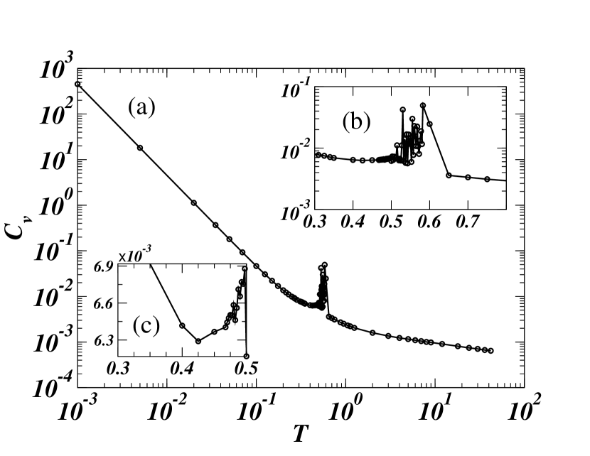
Figure 1: Specific heat as function of temperature for a confined L-J system with $N=515$ particles and an effective filling fraction $\phi\simeq 56\%$. Zooms of the specific heat is represent in the box b) and c).

Considering the behavior of the specific heat as function of temperature, as shown in fig. (1a), we observe a high and narrow peak, which we ascribe to a first order phase transition for $T\approx 0.5$. Notice that in the phase transition region we have relevant fluctuations, as can be observed in fig. (1c). Also we observe a modification on SH for temperatures between $0.4\lesssim T\lesssim 0.5$ (fig. 1b), this feature in the SH might be attributed to a pre-melting region.

In order to better describe the phase transitions in the system, we also estimate the self-diffusion coefficient in the system as a function of the temperature. To do so, the mean squared displacement (MSD) $\left\langle\Delta R^{2}\right\rangle$ of particles as function of the performed MC steps were fitted to a linear law. In fig. (6d) we show some representative cases of this fitting procedure. From the slope the $\left\langle\Delta R^{2}\right\rangle$ vs. the number of Montecarlo steps the diffusion coefficient is extracted. Since we take the averaged $\left\langle\Delta R^{2}\right\rangle$ considering all the particles at the same foot, we have a spatial average of the diffusion coefficient. One might expect to find strong inhomogeneities and anisotropy leading to an inhomogeneous diffusion tensor instead of the averaged scalar values we obtain with our procedure. Nevertheless, we shall see that this averaged diffusion constant suffices to identify phase transitions and a dynamical phase switching regime in our system.

In fig. (2) we plot the diffusion coefficient ($D$) as a function of temperature for three different systems with different number of particles and different volumes, while keeping a constant number density. We observe that the diffusion coefficient, for this scale, does not depend of the size of the system.

Three regions can be identified in fig. (2). In the first region, for normalized temperatures $T\lesssim 0.4$, the structure is crystalline and diffusion is strongly inhibited. This fact is compatible with a pure solid phase. The diffusion coefficient grows with temperature at an approximately constant rate in the range $0.4\lesssim T\lesssim 0.5$ (See fig. 2b). This apparent increase in $D$ signals a pre-melting. It is worth noticing that this region does not correspond to any remarkable feature in the specific heat. The slope of the diffusion constant shows a strong increase at about $T\simeq 0.5$, this kink in the diffusion coefficient curve corresponds to the peak in the specific heat.

In summary, we can establish a phase landscape in which, we identify a pre-melting region that starts at $T\simeq 0.4$, and a (solid-liquid) phase transition at $T\simeq 0.5$. In the following sections we shall focus on the behavior of the system in the phase transition region.

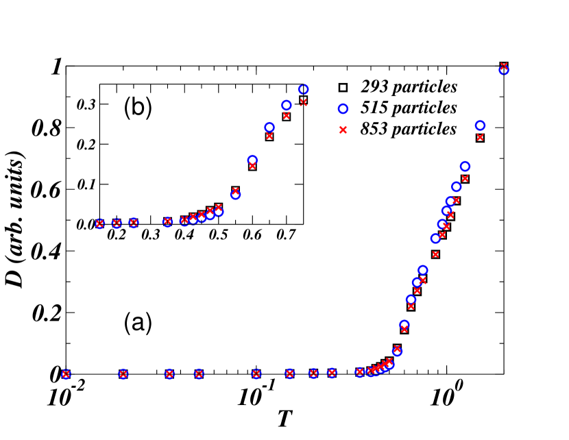
Figure 2: (Color online) a) Diffusion coefficient as a function of the temperature, for three different system sizes of the system at constant particle density. b) Zoom of the same plot in the range $0.15<T<0.75$.

III Phase switching

In fig. (3) we represent the particle energy as function of the MC steps for temperature $T=0.53625$, which corresponds to a temperature in the phase transition region. The system at this temperature oscillates between a lower and a higher value of energy. This bistable energy behavior is the responsible for the fluctuations in the SH. Despite the large number of MC steps used in the sampling, we observe in fig. 3 that the number of high and low energy regions is relatively reduced. Hence, if we calculate the SH through the energy fluctuations of internal energy, large fluctuations due to finite sampling is expected as observed in fig. (1c).

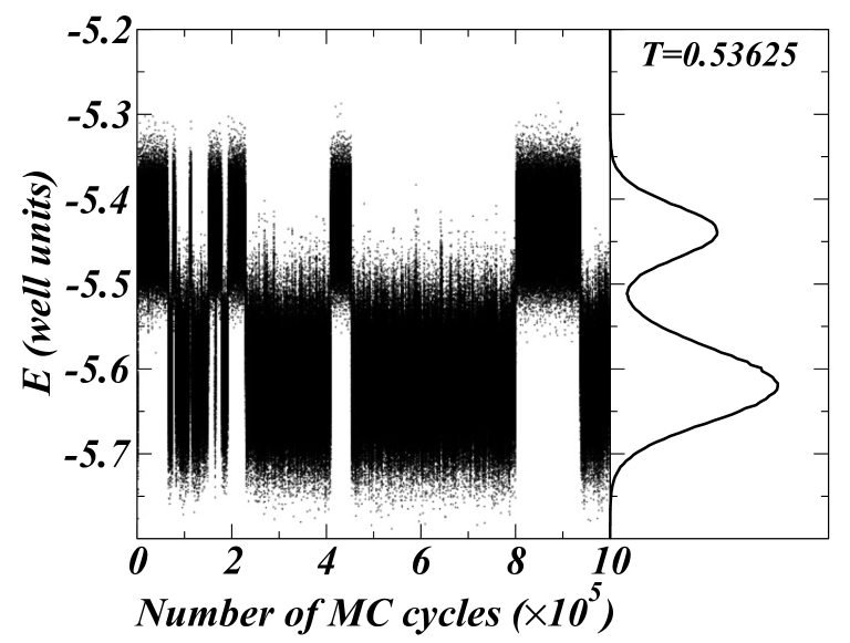
Figure 3: a) Energy sampling of a confined L-J system during a full MC run at a temperature $T=0.53625$, corresponding to a phase-switching region. b) Energy histogram obtained from the MC sampling in a).

Representing the internal energy histogram as function of the temperature, shown in fig. (4), we can identify an energy gap for temperatures at the phase transition. The transition between solid and liquid is not smooth with phase coexistence between two states. Instead, the system switches between this two phases, with abrupt modifications in a small number of MC cycles. In the phase transition, when the particles exhibit a low energy configuration, the system is in the solid phase. For higher energies, the system is in the liquid phase.

One might expect to find intermediate energetic states in the sampling. If both phases coexist the system might switch, or smoothly evolve, among a multitude of different closely spaced energetic states. Nevertheless in all the examined cases the system exclusively switches between two well defined states.

In fact one might expect phase coexistence for larger systems, however, it seems that the size of the current system is small enough to preclude phase coexistence. Apparently the system is so small that a nucleation bubble fills the entire available volume.

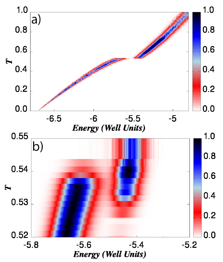
Figure 4: (Color online) a) Colormap showing the energy distribution functions as a function of the temperature. b) Zoom in the region corresponding to the solid-liquid phase transition.

In order to better understand the geometrical and dynamical properties of the system in the phase switching region, we observe that the system remains in either the lower or the upper energy branches for a sufficient amount of time (MC steps) to consider both the structural (pair correlation function) or dynamical (self-diffusion constant) properties in well defined phases.

So far we focused our attention to a system with high number density (effective filling fraction $\phi\simeq 56\%$). Since the interaction potential, although possessing a strong repulsive core, is not a hard-core one, we expect that this behavior can be maintained down to lower densities. We have performed several MC runs on a system with an effective filling fraction $\phi=45\%$ obtaining similar results for the $C_{v}$ as a function of temperature and a finite phase transition region. In fig. (5a), the SH as a function of $T$ is represented. In analogy with previous results, the SH curve shows different areas separated by a narrow peak at the phase transition region . Again, the SH in this region strongly fluctuates due to the finite sampling.

In fig. (5b) we plot an energy sampling analogous to the one appearing in fig. (3a). In this case the temperature is $T=0.485$, corresponding to the maximum of the SH peak. This energy sampling suggests that at this lower density, the phase systems also might switch between two different dynamical states. However the switching apparently happens at a much lower rate than in the previous case. Notice that in this case we performed $\sim 1.5\times 10^{9}$ MC steps to detect one switching event in the energy, while in fig. (3a) several events were detected using much less MC steps. Hence, although extensive simulations would be required, we conjecture that the dynamical behavior presented in this work might be found for any high enough density. The exact meaning of high enough density can not be explicitly given with the available data. In the remainder of this paper, we shall deal only with $\phi=0.56$ systems.

Using much larger systems might allow for the appearance of more than two energy levels and diffusion constants. As a result, the system would evolve with its size to a regime in which actual phase coexistence instead of phase switching takes place.

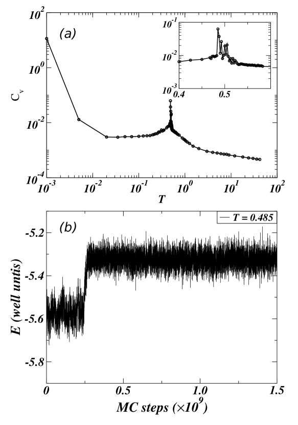
Figure 5: a) Specific heat as function of temperature for a confined L-J system with $N=515$ particles and an effective filling fraction $\phi\simeq 45\%$. Zooms of the specific heat is represent in the inset. b) Energy sampling for the same system during a full MC run at a temperature $T=0.485$, corresponding to a phase-switching region.

III.1 Dynamical properties in the switching regime

Regarding dynamical properties, in fig. (6a-c) we plot the self-diffusion constant as a function of temperature much in the same way as done in fig. 2. In this case, we have split the statistical ensemble in two different sets for temperatures in the phase switching region, one corresponding to the high energy branch (liquid phase), and the other one corresponding to lower energy branch (solid phase). In fig. (6c) it appears evident that the diffusion coefficients corresponding to both phases can differ by a large amount. In the case under study, the diffusion constant differs by a factor 3 between phases at the same temperature.

In fig. (6d) we show several examples of the evolution of the mean squared displacement as a function of the number of MC steps. In all the examined cases, the maximum root mean squared value is well below the radius of the confining sphere, hence we do not expect saturation effects due to confinement. Nevertheless, at higher temperatures and long simulation times, the MSD tends to saturate after a purely diffusive region as expected (not shown for the sake of brevity).

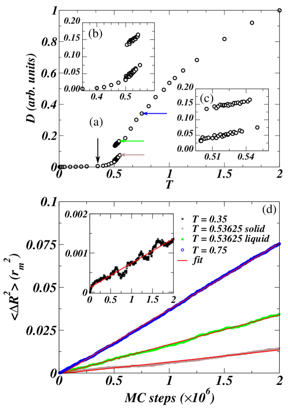
Figure 6: a) Self-diffusion coefficient for a 515 particle system as a function of temperature. Arrows indicate the points corresponding to data in panel d. b) Zoom of the self-diffusion coefficient in the range $0.35\leq T\leq 0.6$. c) Self-diffusion coefficients as a function of temperature obtained for the liquid phase (upper branch) and the solid phase (lower branch) in the region of phase-switching. d) Mean squared displacement as a function of MC steps for different data points shown in a) as indicated by the arrows of the corresponding color. Red lines indicate the linear fit from whose slope the diffusion coefficient is extracted.

III.2 Geometrical properties in the switching regime

Regarding geometrical properties of both phases at the phase switching region, we have studied the radial distribution function $g\left(r\right)$ Percus:1958wv (47, 48). This function is defined as the ratio of the average number density at a distance $r$ from one particle to the averaged number density of an hypothetical, fully uncorrelated, system. Hence, the radial distribution function describes the correlation in the interparticle distance in the system. Again, we can distinguish the statistical sampling in two sets associated with upper and lower energy branches in the phase switching region. Contrary to the behavior of the diffusion constants, the radial distribution function in the upper and lower energy branches is very similar. In fig. 7 we represent the $g\left(r\right)$ for the configurations at both the liquid and solid phase at a fixed temperature. The only marked difference is the indicated split-second peak of $g\left(r\right)$ which for bulk packings of hard spheres is a known signature of a solid phase Donev_2005 (42, 49). Other than that the radial distribution functions $g\left(r\right)$ remain nearly identical when the switching from solid to liquid phases and a clear identification of different phases through structural measurements is therefore much less sensitive than through dynamical measurements (eg. self-diffusion constants) in strongly confined systems.

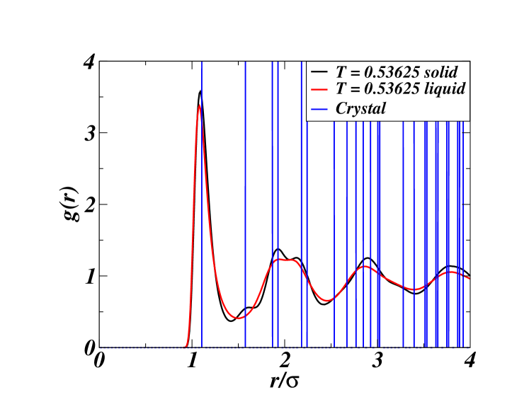
Figure 7: (Color online) Radial distribution function $g\left(r\right)$ obtained at a fixed temperature in the phase switching region ($T\simeq 0.53$) for both the solid (black line) and liquid (red line) phases. Blue vertical lines correspond to a perfect FCC crystal.

IV Conclusion

In summary, we have studied the self-diffusion in a strongly confined Lennard-Jones system. For small clusters, of the order of a few hundreds of particles, instead of phase coexistence the system present dynamic phase switching between solid-like and liquid-like amorphous phases. We found that the self-diffusion coefficient of the liquid-like phase in the phase-switching region can be up to a factor of three larger than the one associated to the solid phase. Interestingly, although the radial distribution functions are nearly the same a split-second peak is observed as a subtle structural signature of transient solid phase.

References

References

- (1) P. Pawlow, Z. Phys. Chem. 65, 1 (1909).
- (2) T. L. Hill, Thermodynamics of Small Systems (Benjamin, New York, 1963).
- (3) J. P. Hansen, and I. R. McDonald, Theory of Simple Liquids (Academic Press, Amsterdam, 2006).
- (4) J. N. Israelachvili, Theory of Simple Liquids (Academic Press, London, 1991).
- (5) B. Bhushan, J. N. Israelachvili, and U. Landman, Nature 374, 607 (1995).
- (6) S. Granick, Science 253, 1374 (1991).
- (7) J. Klein, and E. Kumacheva, Science 269, 816 (1995).
- (8) D. J. Wales, Science 271, 925 (1996).
- (9) J. J. Erpenbeck, and W. W. Wood, Phys. Rev. A 43, 4254 (1991).
- (10) P. A. Thompson, G. S. Grest, and M. O. Robbins, Phys. Rev. Lett. 68, 3448 (1992).
- (11) J. Gao, W. D. Luedtke, and U. Landman, Phys. Rev. Lett. 79, 705 (1997).
- (12) J. Mittal, T. M. Truskett, J. R. Errington, and G. Hummer, Phys. Rev. Lett. 100, 145901 (2008).
- (13) H. Matsubara, F. Pichierri, and K. Kurihara, Phys. Rev. Lett. 109, 197801 (2012).
- (14) L. D. Gelb, K. E. Gubbins, R. Radhakrishnan, and M. Sliwinska-Bartkowiak, Rep. on Prog. in Phys. 62, 1573 (1999).
- (15) R. Evans, and P. Tarazona, Phys. Rev. Lett. 52, 557 (1984).
- (16) M. Köber, E. Sahagún, P. García-Mochales, F. Briones, M. Luna, and J. J. Sáenz, Small 6, 2725 (2010).
- (17) C. Briant and J. Burton, J. Chem. Phys. 63, 2045 (1975).
- (18) P. Buffat and J.-P. Borel, Phys. Rev. A 13, 2287 (1976).
- (19) R. S. Berry, J. Jellinek, and G. Natanson, Phys. Rev. A 30, 919 (1984).
- (20) J. D. Honeycutt and H. C. Andersen, J. Phys. Chem. 91, 4950 (1987).
- (21) R. S. Berry, T. L. Beck, H. L. Davis, and J. Jellinek, Advances in Chemical Physics: Evolution of Size Effects in Chemical Dynamics, Part 2 70 (John Wiley & Sons,1988).
- (22) F. Ercolessi, W. Andreoni, and E. Tosatti, Phys. Rev. Lett. 66, 911 (1991).
- (23) M. Schmidt, R. Kusche, B. von Issendorff, and H. Haberland, Nature 393, 238 (1998).
- (24) F. Baletto and R. Ferrando, Rev. of Mod. Phys. 77, 371 (2005).
- (25) J. Mittal, J. R. Errington, and T. M. Truskett, Phys. Rev. Lett. 96, 177804 (2006).
- (26) Y. Rosenfeld, Phys. Rev. A 15, 2545 (1977).
- (27) T. S. Ingebrigtsen, J. R. Errington, T. M. Truskett, and J. C. Dyre, Phys. Rev. Lett. 111, 235901 (2013).
- (28) S. Auer, D. Frenkel, Nature 409, 6823 (2001).
- (29) K. N. Pham, S. U. Egelhaaf, P. N. Poon, C. K. Wilson, Phys. Rev. E 69, 011503 (2004).
- (30) P. Labastie and R. L. Whetten, Phys. Rev. Lett. 65, 1567 (1990).
- (31) D. J. Wales and R. S. Berry, Phys. Rev. Lett. 73, 2875 (1994).
- (32) C. L. Cleveland, U. Landman, and W. D. Luedtke, J. Phys. Chem. 98, 6272 (1994).
- (33) D. Schebarchov and S. Hendy, J. Chem. Phys. 123, 104701 (2005).
- (34) N. Quirke, Mol. Simulation 1, 249 (1988).
- (35) W. Polak, European Phys. J. D 40, 231 (2006).
- (36) T. L. Beck and T. L. I. Marchioro, J. Chem. Phys. 93, 1347 (1990).
- (37) I.-C. Yeh and G. Hummer, J. Phys. Chem. B 108, 15873 (2004).
- (38) C. L. Cleveland, W. D. Luedtke, and U. Landman, Phys. Rev. B 60, 5065 (1999).
- (39) D. P. Landau and K. Binder, A Guide to Monte Carlo Simulation in Statistical Physics (World Scientific, Singapure, 1994).
- (40) H. Huitema and J. P. Van der Eerden, J. Chem. Phys. 110, 3267 (1999).
- (41) M.L. A. Donev, S. Torquato, and F. H. Stillinger, Phys. Rev. E 71, 011105 (2005).
- (42) K. Nygård, R. Kjellander, S. Sarman, S. Chodankar, E. Perret, J. Buitenhuis, and J. F. van der Veen, Phys. Rev. Lett. 108, 037802 (2012).
- (43) R. Kimmich, NMR: tomography, diffusometry, relaxometry (Springer, Berlin, 1997).
- (44) E. L. Elson and D. Magne, Biopolymers 13, 1 (1974).
- (45) F. Wang and D. P. Landau, Phys. Rev. E 64, 056101 (2001).
- (46) J. K. Percus and G. J. Yevick, Phys. Rev. 110, 1 (1958).
- (47) M. S. Wertheim, Phys. Rev. Lett. 10, 321 (1963).
- (48) A. J. Liu, S. R. Nagel, The Jamming Scenario: An Introduction and Outlook (Oxford University Press, Oxford, 2010).