Resolving sets for breaking symmetries of graphs

Abstract

This paper deals with the maximum value of the difference between the determining number and the metric dimension of a graph as a function of its order. Our technique requires to use locating-dominating sets, and perform an independent study on other functions related to these sets. Thus, we obtain lower and upper bounds on all these functions by means of very diverse tools. Among them are some adequate constructions of graphs, a variant of a classical result in graph domination and a polynomial time algorithm that produces both distinguishing sets and determining sets. Further, we consider specific families of graphs where the restrictions of these functions can be computed. To this end, we utilize two well-known objects in graph theory: $k$-dominating sets and matchings.

1 Introduction and preliminaries

Every resolving parameter conveys useful information about the behavior of distances in a graph. Thus, considering several of those parameters together provides stronger properties of the underlying graph, which is the reason for studying the relations among them. Indeed, much effort has gone into relating metric dimension and other similar invariants including partition dimension [9, 45], upper dimension [12, 26], and resolving number [13, 36], to name but a few. Combining metric dimension and determining number allows us to obtain not only metric properties of graphs but also an extra information about their symmetries. However, there are no many papers dealing with the connection between these two parameters: the determining number of a graph is bounded above by its metric dimension [7, 22]. This prompts the following question posed by Boutin [7]: Can the difference between the determining number and the metric dimension of a graph be arbitrarily large? To deal with this question, which is the main problem of this paper, we next define these parameters.

Let $G$ be a connected graph. Given a set $S\subseteq V(G)$, the stabilizer of $S$ is $\operatorname{Stab}(S)=\{\phi\in\operatorname{Aut}(G):\phi(u)=u,\forall u\in S\}$, and $S$ is a determining set of $G$ if $\operatorname{Stab}(S)$ is trivial. The determining number of $G$, denoted by $\operatorname{Det}(G)$, is the minimum cardinality of a determining set of $G$. A vertex $u\in V(G)$ resolves a pair $\{x,y\}\subseteq V(G)$ if $d(u,x)\neq d(u,y)$, and $S$ is a resolving set of $G$ if every pair of vertices of $G$ is resolved by some vertex of $S$. The metric dimension of $G$, written as $\dim(G)$, is the minimum order of a resolving set of $G$, and a resolving set of size $\dim(G)$ is called a metric basis of $G$.

Determining sets were introduced in 2006 by Boutin [7], and independently by Erwin and Harary [22], who adopted the term fixing set. However, this concept was defined in a more general context in 1971 by Sims [41]: a base of a permutation group of a set is a subset of elements whose stabilizer is trivial. Also in the 1970s, resolving sets were introduced by Harary and Melter [28], and independently by Slater [42]. These two types of sets have been widely studied in the literature because of their multiple applications in very diverse areas. For instance, bases are useful tools for storing and analyzing large permutation groups [5], and resolving sets are utilized for the graph isomorphism problem [3]. We refer the reader to the survey of Bailey and Cameron [4] for more references on these topics.

As it was said before, there is a relationship between the determining number and the metric dimension: every resolving set of a graph $G$ is also a determining set, and consequently $\operatorname{Det}(G)\leq\dim(G)$ [7, 22]. Let $(\dim-\operatorname{Det})(n)$ be the maximum value of $\dim(G)-\operatorname{Det}(G)$ over all graphs $G$ of order $n$. Thus, the computation of this function is equivalent to answer the above-mentioned question asked by Boutin [7] about the difference between our parameters, which is widely studied by Cáceres et al. [8]. Namely, they provide the following bounds.

Proposition 1.1.

[8] For every $n\geq 8$,

$$\lfloor\frac{2}{5}n\rfloor-2\leq({\rm dim}-{\rm Det})(n)\leq n-2.$$

Fundamental to our technique, which lets us improve significatively the above result, are locating-dominating sets. Hence, we next introduce these sets together with the functions $(\lambda-{\rm Det})(n)$ and $\lambda(n)$, for which we have to develop an independent study that is also of interest.

A vertex $u\in V(G)$ distinguishes a pair $\{x,y\}\subseteq V(G)$ if either $u\in\{x,y\}$ or $N(x)\cap\{u\}\neq N(y)\cap\{u\}$, and a set $D\subseteq V(G)$ is a distinguishing set of $G$ if every pair of $V(G)$ is distinguished by some vertex of $D$. If $D$ is also a dominating set of $G$, i.e., $N(x)\cap D\neq\emptyset$ for every $x\in V(G)\setminus D$, then we say that $D$ is a locating-dominating set of $G$. The minimum cardinality of a locating-dominating set of $G$ is its locating-domination number, denoted by $\lambda(G)$.

Distinguishing sets were defined by Babai [3] when constructing canonical labelings for the graph isomorphism problem, while Slater [43] introduced locating-dominating sets in the context of domination. However, these two concepts are in essence the same: one can easily check that every distinguishing set becomes a dominating set by adding at most one vertex. This implies the following observation.

Remark 1.2.

For any distinguishing set $D$ of a graph $G$, $\lambda(G)\leq|D|+1$.

Every locating-dominating set of $G$ is clearly a resolving set, and so ${\rm Det}(G)\leq{\rm dim}(G)\leq\lambda(G)$ which leads us to pose a similar question to that of Boutin [7] but concerning the difference $\lambda(G)-\operatorname{Det}(G)$. Thus, let $(\lambda-{\rm Det})(n)$ and $\lambda(n)$ be the maximum values of, respectively, $\lambda(G)-{\rm Det}(G)$ and $\lambda(G)$ over all graphs $G$ of order $n$. Although the function $\lambda(n)$ equals $n-1$ (just take the complete graph $K_{n}$), we need to define it because we shall consider a non-trivial restriction of $\lambda(n)$ which is quite useful throughout the paper. Therefore, it is straightforward that

$$({\rm dim}-{\rm Det})(n)\leq(\lambda-{\rm Det})(n)\leq\lambda(n)=n-1.$$ (1)

This paper undertakes a study on the function $({\rm dim}-{\rm Det})(n)$ which requires to develop a parallel study on $(\lambda-\operatorname{Det})(n)$ and the function $\lambda_{|_{\mathcal{C}^{*}}}(n)$ described in Section 3. We thus start by constructing appropriate families of graphs which provide new lower bounds on $({\rm dim}-{\rm Det})(n)$ and $(\lambda-\operatorname{Det})(n)$, improving the lower bound of Proposition 1.1 by Cáceres et al. [8]. Further, we conjecture that these are precisely the exact values of these functions. To improve the upper bound, we require a more sophisticated method which uses the locating-domination number of twin-free graphs, namely the function $\lambda_{|_{\mathcal{C}^{*}}}(n)$. Indeed, we first prove that this function is an upper bound on $(\dim-\operatorname{Det})(n)$ and $(\lambda-\operatorname{Det})(n)$, and then conjecture a presumable value of $\lambda_{|_{\mathcal{C}^{*}}}(n)$ which will be supported through the paper.

Subsequently, we obtain two explicit upper bounds on $\lambda_{|_{\mathcal{C}^{*}}}(n)$ in Sections 4 and 5, respectively. For the first one, we give a different version of a classical theorem in domination theory due to Ore [39]. This version leads us to a series of relationships between the locating-domination number and classical graph parameters in twin-free graphs, similar to the relations established among other domination parameters in many papers (see [30] for a number of examples). Besides their own interest, these relations yield a first explicit bound on $\lambda_{|_{\mathcal{C}^{*}}}(n)$ by using a nice Ramsey-type result due to Erdős and Szekeres [21].

The second upper bound that we provide on $\lambda_{|_{\mathcal{C}^{*}}}(n)$ is, until now, the best bound known on $(\dim-\operatorname{Det})(n)$. It is obtained from the greedy algorithm described in Section 5 which produces both distinguishing sets and determining sets of bounded size in polynomial time. Hence, we also obtain a bound on the determining number of a twin-free graph.

Finally, we devote the last two sections to the family of graphs not containing the complete bipartite graph $K_{2,k}$ as a subgraph. Concretely, we provide bounds and exact values of our main functions restricted to graphs without the cycle $C_{4}$ as a subgraph in Section 6. For this purpose, we obtain relationships between the locating-domination number of a twin-free graph and other two well-known parameters: the $k$-domination number and the matching number. Hence, we get bounds on these two invariants similar to other relations provided in a number of papers (see Section 6 for the details). Furthermore, we compute the restrictions of $(\dim-\operatorname{Det})(n)$ and $(\lambda-\operatorname{Det})(n)$ to the family of trees in Section 7, thereby closing the study initiated by Cáceres et al. [8] on this class of graphs.

2 Lower bounds on $(\dim-\operatorname{Det})(n)$ and $(\lambda-\operatorname{Det})(n)$

The question raised by Boutin [7] arose from the fact that all graphs $G$ where she computed $\dim(G)-\operatorname{Det}(G)$ have a very small value of this difference. Thus, Cáceres et al. [8] found a family of graphs with constant determining number and metric dimension with linear growth: the wheel graphs $W_{1,n}=K_{1}+C_{n}$ for which $\dim(W_{1,n})-\operatorname{Det}(W_{1,n})=\lfloor\frac{2}{5}n\rfloor-2$. This implies a lower bound on the maximum value of this difference, i.e., a lower bound on the function $(\dim-\operatorname{Det})(n)$ (see Proposition 1.1 above). In this section, we improve this bound and also give a lower bound on $(\lambda-\operatorname{Det})(n)$. To do this, we next provide two appropriate families of graphs.

For an integer $r\geq 6$, let $T_{r}$ be a path $(u_{1},...,u_{r})$ with a pendant vertex $u_{0}$ adjacent to $u_{3}$. The corona product $G\circ K_{1}$ is the graph obtained from attaching a pendant vertex to every vertex of any graph $G$. Let $G_{r}=T_{r}\circ K_{1}$ and let $H_{r}$ be the graph resulting from $G_{r}$ by attaching a pendant vertex $v_{0}^{\prime}$ to $u_{0}$ (see Figure 1).

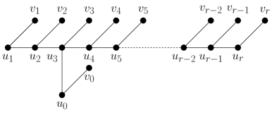
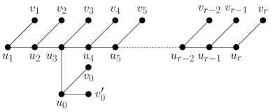
(a)	(b)

Figure 1: The graphs (a) $G_{r}$ and (b) $H_{r}$.

The following lemma gives some evaluations of the main parameters considered in the paper for the graphs $G_{r}$, $H_{r}$ and their complements $\overline{G}_{r}$ and $\overline{H}_{r}$. These are the key tools for proving Theorem 2.2 below.

Lemma 2.1.

For every $r\geq 6$, the following statements hold:

1. $\operatorname{Det}(G_{r})=0$ and $\operatorname{Det}(H_{r})=1$.

2. $\dim(\overline{G}_{r})=r$ and $\dim(\overline{H}_{r})=r+1$.

3. $\lambda(G_{r})=r+1$ and $\lambda(H_{r})=r+2$.

Proof.

Let $V(G_{r})=\{u_{0},...,u_{r},v_{0},...,v_{r}\}$ and $E(G_{r})=E(T_{r})\cup\{\{u_{i},v_{i}\}:0\leq i\leq r\}$. Also, let $V(H_{r})=V(G_{r})\cup\{v_{0}^{\prime}\}$ and $E(H_{r})=E(G_{r})\cup\{\{u_{0},v_{0}^{\prime}\}\}$. The three statements are proved one by one.

1. $\operatorname{Det}(G_{r})=0$ since the automorphism group of $G_{r}$ is trivial. On the other hand, $\operatorname{Aut}(H_{r})=\{id_{H_{r}},f\}$ where $f$ interchanges $v_{0}$ and $v_{0}^{\prime}$, and fixes any other vertex. Hence, $S=\{v_{0}\}$ is clearly a minimum determining set of $H_{r}$ and so $\operatorname{Det}(H_{r})=1$.

2. Observe that every resolving set $S$ of $\overline{G}_{r}$ contains either $u_{i}$ or $v_{i}$ for every $0\leq i\leq r$, except for at most one. Otherwise, there are $u_{i},v_{i},u_{j},v_{j}\not\in S$ for some $i\neq j$, which implies that $d(u,v_{i})=1=d(u,v_{j})$ for every $u\in S$ and so $S$ is not a resolving set of $\overline{G}_{r}$; a contradiction. Therefore, $\dim(\overline{G}_{r})\geq r$ and equality is given by the set $S=\{u_{0},u_{1},...,u_{r-2},u_{r}\}$ which is a metric basis of $\overline{G}_{r}$.

   The same arguments apply to prove that $S\cup\{v_{0}^{\prime}\}$ is a metric basis of $\overline{H}_{r}$, and then $\dim(\overline{H}_{r})=r+1$.

3. Let $D$ be a locating-dominating set of $G_{r}$. Note that either $u_{i}$ or $v_{i}$ belongs to $D$ for every $0\leq i\leq r$ (otherwise $N(v_{i})\cap D=\emptyset$ and so $D$ is not a dominating set of $G_{r}$; a contradiction). Hence, $\lambda(G_{r})\geq r+1$ and equality holds since $D=\{u_{0},...,u_{r}\}$ is clearly a locating-dominating set of $G_{r}$.

   Arguing as above, we can check that $D\cup\{v_{0}^{\prime}\}$ is a minimum locating-dominating set of $H_{r}$ and so $\lambda(H_{r})=r+2$.

∎

With these values in hand, we next obtain lower bounds on $(\dim-\operatorname{Det})(n)$ and $(\lambda-\operatorname{Det})(n)$ which in particular improve Proposition 1.1 above due to Cáceres et al. [8].

Theorem 2.2.

For every $n\geq 14$,

$$(\dim-\operatorname{Det})(n)\geq\lfloor\frac{n}{2}\rfloor-1\qquad and\qquad(\lambda-\operatorname{Det})(n)\geq\lfloor\frac{n}{2}\rfloor.$$

Proof.

To prove that $(\dim-\operatorname{Det})(n)\geq\lfloor\frac{n}{2}\rfloor-1$ we only need to show that, for every $n\geq 14$, there exists a graph $G$ of order $n$ such that $\dim(G)-\operatorname{Det}(G)=\lfloor\frac{n}{2}\rfloor-1$. If $n$ is even then let $G=\overline{G}_{\frac{n}{2}-1}$. Indeed, $\overline{G}_{\frac{n}{2}-1}$ has order $n$ and Lemma 2.1 yields $\dim(\overline{G}_{\frac{n}{2}-1})-\operatorname{Det}(\overline{G}_{\frac{n}{2}-1})=\lfloor\frac{n}{2}\rfloor-1$ (note that $\operatorname{Det}(G)=\operatorname{Det}(\overline{G})$ holds for any graph $G$ since $\operatorname{Aut}(G)=\operatorname{Aut}(\overline{G})$). Otherwise, $n$ is odd and we set $G=\overline{H}_{\frac{n-1}{2}-1}$, whose order is $n$ and satisfies $\dim(\overline{H}_{\frac{n-1}{2}-1})-\operatorname{Det}(\overline{H}_{\frac{n-1}{2}-1})=\lfloor\frac{n}{2}\rfloor-1$, by Lemma 2.1.

Considering the graphs $G_{\frac{n}{2}-1}$ (when $n$ is even) and $H_{\frac{n-1}{2}-1}$ (when $n$ is odd), one can use the same arguments as above to show that $(\lambda-\operatorname{Det})(n)\geq\lfloor\frac{n}{2}\rfloor$. ∎

In the remainder of the paper, we shall exhibit wide classes of graphs where the restrictions of $(\dim-\operatorname{Det})(n)$ and $(\lambda-\operatorname{Det})(n)$ do not exceed $\frac{n}{2}$. Thus, there are reasons to believe that the bounds given above are the exact values of these functions. We state this as a conjecture.

Conjecture 1.

There exists a positive integer $n_{0}$ such that, for every $n\geq n_{0}$,

$$(\dim-\operatorname{Det})(n)=\lfloor\frac{n}{2}\rfloor-1\qquad and\qquad(\lambda-\operatorname{Det})(n)=\lfloor\frac{n}{2}\rfloor.$$

3 An upper bound on $(\dim-\operatorname{Det})(n)$ and $(\lambda-\operatorname{Det})(n)$

In this section, we assemble all the necessary machinery in order to prove that $(\dim-\operatorname{Det})(n)$ and $(\lambda-\operatorname{Det})(n)$ are bounded above by the function $\lambda_{|_{\mathcal{C}^{*}}}(n)$ which is the maximum value of $\lambda(G)$ over all twin-free graphs $G$ of order $n$ (see Theorem 3.6). The proof requires basically the following two ideas: the construction of a twin-free graph $\widetilde{G}$ from an arbitrary graph $G$ based on the so called twin graph described in Subsection 3.1, and the relationship between $\lambda(G)$ and $\lambda(\widetilde{G})$ given in Subsection 3.2.

3.1 The twin graph $G^{*}$

For a graph $G$, the twin graph $G^{*}$ is obtained from $G$ by identifying vertices with the same neighborhood. This construction and any of its variations (depending on the choice of closed and/or open neighborhoods) completely characterize the original graph, which is the reason why they have been considered for solving many problems in graph theory (see for instance [29, 31, 35, 40]). In this subsection, we provide some properties of $G^{*}$ and a bound on $\operatorname{Det}(G)$ in terms of $|V(G^{*})|$, each of which is useful in the paper. The twin graph is formally defined as follows.

Two different vertices $u,v\in V(G)$ are twins if $N(u)=N(v)$ or $N[u]=N[v]$, i.e., no vertex of $V(G)\setminus\{u,v\}$ distinguishes $\{u,v\}$. It is proved in [35] that this definition induces an equivalence relation on $V(G)$ given by $u\equiv v$ if and only if either $u=v$ or $u$ and $v$ are twins. Thus, let $u^{*}=\{v\in V(G):u\equiv v\}$ and consider the partition $u_{1}^{*},...,u_{r}^{*}$ of $V(G)$ induced by this relation, where every $u_{i}$ is a representative of $u_{i}^{*}$. The twin graph of $G$, written as $G^{*}$, has vertex set $V(G^{*})=\{u_{1}^{*},...,u_{r}^{*}\}$ and edge set $E(G^{*})=\{\{u_{i}^{*},u_{j}^{*}\}:\{u_{i},u_{j}\}\in E(G)\}$. Note that, for every $x\in V(G)$, we shall consider $x^{*}$ as a class in $V(G)$, as well as a vertex of $G^{*}$. The twin graph $G^{*}$ has the following properties.

Lemma 3.1.

[35] For every graph $G$, the following statements hold:

1. The graph $G^{*}$ is independent of the choice of the representatives $u_{i}$, i.e.,

   $$\{u_{i}^{*},u_{j}^{*}\}\in E(G^{*})\qquad\Longleftrightarrow\qquad\{x,y\}\in E(G)\quad\forall x\in u_{i}^{*},y\in u_{j}^{*}$$

2. Every class $u_{i}^{*}$ either induces a complete subgraph or is an independent set in $G$.

A vertex $u_{i}^{*}\in V(G^{*})$ is of type $(1)$ if $|u_{i}^{*}|=1$; otherwise $u_{i}^{*}$ is of type $(KN)$. According to Statement 2 of Lemma 3.1, a vertex $u_{i}^{*}$ of type $(KN)$ is of type $(K)$ or $(N)$, depending on weather $u_{i}^{*}$ induces a complete subgraph or is an independent set in $G$. Note that $N[x]=N[y]$ for every $x,y\in u_{i}^{*}$ whenever $u_{i}^{*}$ is of type $(K)$, and $N(x)=N(y)$ for every $x,y\in u_{i}^{*}$ whenever $u_{i}^{*}$ is of type $(N)$. For more properties of $G^{*}$ we refer the reader to [35].

Now, we give two lemmas considering the twin graph $G^{*}$ which will be helpful in the remainder of the paper.

Lemma 3.2.

For every graph $G$, no two different vertices $u_{i}^{*},u_{j}^{*}\in V(G^{*})$ of type $(1)$ are twins in $G^{*}$.

Proof.

Since $u_{i}^{*}\neq u_{j}^{*}$ there exists a vertex $u\in V(G)\setminus\{u_{i},u_{j}\}$ distinguishing $\{u_{i},u_{j}\}$. Without loss of generality, assume that $u_{i}\in N_{G}(u)$ and $u_{j}\not\in N_{G}(u)$. Also, observe that $u$ is not contained in $u_{i}^{*}$ or $u_{j}^{*}$ since they are of type $(1)$. Therefore, $u_{i}^{*}\in N_{G^{*}}(u^{*})$ and $u_{j}^{*}\not\in N_{G^{*}}(u^{*})$, which implies that $u_{i}^{*}$ and $u_{j}^{*}$ are not twins in $G^{*}$. ∎

Let $\Omega_{G}=\bigcup_{1\leq i\leq r}u_{i}^{*}\setminus\{u_{i}\}$ which is composed by all but one vertex of every class of type $(KN)$. Clearly, this set has cardinality $n-r$ and satisfies that no two vertices of $V(G)\setminus\Omega_{G}$ are twins in $G$. Observe that $\Omega_{G}$ is also independent of the choice of the representatives $u_{i}$. Using this set, we can prove the following result.

Lemma 3.3.

Let $G$ be a graph of order $n$ such that $G^{*}$ has order $r$. Then,

$$\operatorname{Det}(G)\geq n-r.$$

In particular, $\lambda(G)-\operatorname{Det}(G)\leq r-1$.

Proof.

Let $u_{i}^{*}$ be a class of type $(KN)$ in $V(G)$. For each $x,y\in u_{i}^{*}$, let $f\in\operatorname{Aut}(G)$ fixing every vertex of $G$ but $x$ and $y$, which are interchanged. Obviously, $f\in\operatorname{Stab}(V(G)\setminus\{x,y\})$ and $f\neq id_{G}$. Hence, every determining set $S$ of $G$ contains either $x$ or $y$. It follows that $S$ contains all but one vertex of each class of type (KN), i.e., $|\Omega_{G}|=n-r$ vertices. Therefore, $\operatorname{Det}(G)\geq n-r$ and combining this with $\lambda(G)\leq n-1$ yields $\lambda(G)-\operatorname{Det}(G)\leq r-1$. ∎

3.2 Using locating-dominating sets of twin-free graphs

In this subsection, we provide an upper bound on the functions $(\dim-\operatorname{Det})(n)$ and $(\lambda-\operatorname{Det})(n)$ based on the locating-domination number of twin-free graphs. These graphs are important for their own sake [1, 2, 10, 44], and also for their many applications to other problems in graph theory [25, 29, 38]. Here, we construct a twin-free graph $\widetilde{G}$ for every graph $G$ (whenever $G^{*}\not\cong K_{2}$) in such a way that we can obtain locating-dominating sets of $G$ from those of $\widetilde{G}$. This construction and the relation between $\lambda(G)$ and $\lambda(\widetilde{G})$ given in Lemma 3.5 below are the key tools to prove the above-mentioned bound on $(\dim-\operatorname{Det})(n)$ and $(\lambda-\operatorname{Det})(n)$ (see Theorem 3.6).

A graph $G$ is twin-free if it does not contain twin vertices. Observe that $G^{*}$ is not necessarily twin-free (see for instance Figures 2(a) and 2(b)). However, we shall use this graph to associate a twin-free graph $\widetilde{G}$ to $G$. Indeed, let $\widetilde{G}$ be the graph obtained from $G^{*}$ by attaching a pendant vertex to every $u_{i}^{*}\in V(G^{*})$ of type $(KN)$ whenever $u_{i}^{*}$ has some twin in $G^{*}$ (see Figure 2(c)). Thus, let us denote $V(\widetilde{G})=V^{*}\cup\mathcal{L}$, where $V^{*}=\{u_{1}^{*},...,u_{r}^{*}\}$ and $\mathcal{L}$ is the set of pendant vertices adjacent to vertices of $V^{*}$. Note again that, for every $x\in V(G)$, $x^{*}$ denotes a class in $V(G)$, a vertex of $V(G^{*})$, as well as a vertex of $V^{*}\subseteq V(\widetilde{G})$.

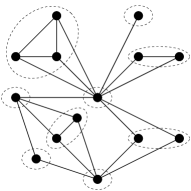
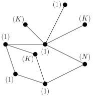
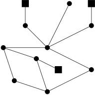
(a)				(b)				(c)

Figure 2: (a) A graph $G$ and its classes in $G^{*}$, (b) the twin graph $G^{*}$ and (c) the associated graph $\widetilde{G}$.

We next provide two technical lemmas about $\widetilde{G}$ which are useful in the proof of Theorem 3.6 and other proofs of this paper.

Lemma 3.4.

Let $G$ be a graph of order $n$ such that $G^{*}$ is not isomorphic to $K_{2}$. Then, the graph $\widetilde{G}$ has order $\widetilde{n}\leq n$ and is twin-free.

Proof.

When obtaining $G^{*}$ from $G$, we ”lose” at least one vertex for each class of type $(KN)$ since they contain at least two vertices. Thus, every time we attach a pendant vertex to a vertex of type $(KN)$ for constructing $\widetilde{G}$ from $G^{*}$, we do not exceed the order of $G$. Hence, $\widetilde{n}\leq n$.

Now, we prove that $\widetilde{G}$ is twin-free. On the contrary, suppose that $\widetilde{G}$ has a pair of twins, say $u,v\in V(\widetilde{G})$. If $u,v\in V^{*}$ then it is easy to see that they are also twins in $G^{*}$. Hence, at least one of them is of type $(KN)$, by Lemma 3.2, and so they are distinguished in $\widetilde{G}$ by the corresponding pendant vertex of $\mathcal{L}$; a contradiction. Moreover, no two pendant vertices of $\mathcal{L}$ are twins since they are adjacent to different vertices of $V^{*}$. Therefore, we can assume that $u\in V^{*}$ and $v\in\mathcal{L}$.

Let $u=u_{i}^{*}$ and let $u_{j}^{*}$ be such that $N_{\widetilde{G}}(v)=\{u_{j}^{*}\}$ for some $1\leq i,j\leq r$. Since $u$ and $v$ are twins, we can assume that $N_{\widetilde{G}}(u)=N_{\widetilde{G}}(v)=\{u_{j}^{*}\}$ (otherwise $N_{\widetilde{G}}[u]=N_{\widetilde{G}}[v]=\{v,u_{j}^{*}\}$ and so $\widetilde{G}\cong K_{2}$ since $\widetilde{G}$ must be connected, which implies that $G^{*}\cong K_{1}$; a contradiction since $G^{*}\cong K_{1}$ implies that $\widetilde{G}\cong K_{1}$). Hence, $u_{i}^{*}\neq u_{j}^{*}$ and, by construction of $\widetilde{G}$, $u_{j}^{*}$ must have a twin in $G^{*}$, say $u_{k}^{*}$. Clearly, $u_{k}^{*}\neq u_{i}^{*}$ (otherwise $u_{i}^{*}$ and $u_{j}^{*}$ are twins in $G^{*}$ and so $G^{*}\cong K_{2}$ since $N_{\widetilde{G}}(u_{i}^{*})=N_{G^{*}}(u_{i}^{*})=\{u_{j}^{*}\}$; a contradiction). Thus, $u_{k}^{*}\in N_{G^{*}}(u_{i}^{*})$ since $u_{j}^{*}$ and $u_{k}^{*}$ are twins and we know that $u_{j}^{*}\in N_{G^{*}}(u_{i}^{*})$ but $N_{\widetilde{G}}(u^{*}_{i})=N_{G^{*}}(u_{i}^{*})=\{u_{j}^{*}\}$, which is a contradiction. ∎

The following lemma establishes a relationship between $\lambda(G)$ and $\lambda(\widetilde{G})$, and is a key result for proving Theorem 3.6.

Lemma 3.5.

Let $G$ be a graph of order $n$ such that $G^{*}$ has order $r$. Then,

$$\lambda(G)\leq\lambda(\widetilde{G})+n-r.$$

In particular, $\lambda(G)-\operatorname{Det}(G)\leq\lambda(\widetilde{G})$.

Proof.

Let $S\subseteq V(\widetilde{G})$ be a minimum locating-dominating set of $\widetilde{G}$. Observe that, for every $u\in V(\widetilde{G})$, there is a unique $u_{i}\in V(G)$ with $1\leq i\leq r$ such that either $u=u_{i}^{*}$ or $N_{\widetilde{G}}(u)=\{u_{i}^{*}\}$ (depending on whether $u\in V^{*}$ or $u\in\mathcal{L}$). Thus, let $\pi(u)$ be such $u_{i}$ and $\pi(S)=\{\pi(u):u\in S\}$. Clearly, the set $\pi(S)$ satisfies $|\pi(S)|\leq|S|=\lambda(\widetilde{G})$ because $\pi(u)=\pi(v)$ whenever $u,v\in S$ with $u\in V^{*}$, $v\in\mathcal{L}$ and $N_{\widetilde{G}}(v)=\{u\}$. Therefore, we will obtain the expected bound by proving that $S^{\prime}=\pi(S)\cup\Omega_{G}$ is a locating-dominating set of $G$ since $|\Omega_{G}|=n-r$.

First, observe that $\pi(u)=u_{i}$ implies that $u_{i}^{*}\subseteq S^{\prime}$ whenever $u\in S$. We claim that $S^{\prime}$ is a distinguishing set of $G$. Indeed, given $x,y\in V(G)\setminus S^{\prime}$, we shall prove that $\{x,y\}$ is distinguished by some vertex of $S^{\prime}$. Obviously, we can assume that $x^{*}\neq y^{*}$ in $G^{*}$ (otherwise either $x$ or $y$ belongs to $\Omega_{G}\subseteq S^{\prime}$; a contradiction since $x,y\in V(G)\setminus S^{\prime}$). Since $S$ is a locating-dominating set of $\widetilde{G}$, then there is $u\in S$ distinguishing $\{x^{*},y^{*}\}$ in $\widetilde{G}$, and we can suppose that $u\neq x^{*}\neq y^{*}$ (otherwise either $u=x^{*}\subseteq S^{\prime}$ or $u=y^{*}\subseteq S^{\prime}$; a contradiction).

If $u\in\mathcal{L}$ then, without loss of generality, let us assume that $x^{*}\in N_{\widetilde{G}}(u)$ and $y^{*}\not\in N_{\widetilde{G}}(u)$. Thus, $\pi(u)=u_{i}$ with $u_{i}^{*}=x^{*}$ and so $x^{*}\subseteq S^{\prime}$; a contradiction with $x\in V(G)\setminus S^{\prime}$. Hence, $u\in V^{*}$ and so $u=u_{i}^{*}$ for some $1\leq i\leq r$, which leads to $\pi(u)=u_{i}\in S^{\prime}$. Assuming that $x^{*}\in N_{\widetilde{G}}(u)$ and $y^{*}\not\in N_{\widetilde{G}}(u)$ (the opposite case is similar), we have that $x\in N_{G}(u_{i})$ and $y\not\in N_{G}(u_{i})$, by Statement 1 of Lemma 3.1, which implies that $u_{i}$ distinguishes $\{x,y\}$. Therefore, $S^{\prime}$ is a distinguishing set of $G$ and a similar analysis shows that it is also a dominating set.

We have just proved that $\lambda(G)\leq\lambda(\widetilde{G})+n-r$, which combined with $\operatorname{Det}(G)\geq n-r$ (see Lemma 3.3) yields $\lambda(G)-\operatorname{Det}(G)\leq\lambda(\widetilde{G})$, as claimed. ∎

For any class of graphs $\mathcal{C}$, we define $(\dim-\operatorname{Det})_{|_{\mathcal{C}}}(n)$, $(\lambda-\operatorname{Det})_{|_{\mathcal{C}}}(n)$ and $\lambda_{|_{\mathcal{C}}}(n)$ as in Section 1 but restricting their domains to the graphs of $\mathcal{C}$. Let $\mathcal{C}^{*}$ be the class of twin-free graphs. Thus, the function $\lambda_{|_{\mathcal{C}^{*}}}(n)$ can be considered for every $n\geq 4$ since $P_{4}$ is clearly the smallest twin-free graph.

We now reach the main result of this section which improves significatively Expression (1).

Theorem 3.6.

For every $n\geq 4$,

$$(\dim-\operatorname{Det})(n)\leq(\lambda-\operatorname{Det})(n)\leq\lambda_{|_{\mathcal{C}^{*}}}(n).$$

Proof.

Since the first inequality is obvious, we only need to show that $(\lambda-\operatorname{Det})(n)\leq\lambda_{|_{\mathcal{C}^{*}}}(n)$. We begin by proving the following two claims.

Claim 1.

For a graph $G$, let $H$ be the graph obtained from $G$ by attaching a pendant vertex $u$ to a vertex $v\in V(G)$. Then, $\lambda(G)\leq\lambda(H)$.

Proof.

Let $S\subseteq V(H)$ be a minimum locating-dominating set of $H$. Clearly, if $u\notin S$ then $S\subseteq V(G)$ is also a locating-dominating set of $G$, and so $\lambda(G)\leq\lambda(H)$. Otherwise $u\in S$ and it is easy to check that $S^{\prime}=(S\setminus\{u\})\cup\{v\}$ is a locating-dominating set of $G$. Therefore, $\lambda(G)\leq|S^{\prime}|\leq\lambda(H)$. ∎

Claim 2.

$\lambda_{|_{\mathcal{C}^{*}}}(n)\leq\lambda_{|_{\mathcal{C}^{*}}}(n+1).$

Proof.

Consider a twin-free graph $G$ of order $n$ such that $\lambda(G)=\lambda_{|_{\mathcal{C}^{*}}}(n)$. To prove the claim, it suffices to find a twin-free graph $H$ of order $n+1$ such that $\lambda(H)\geq\lambda(G)$. Indeed, let $H$ be the graph obtained from $G$ by attaching a pendant vertex $u$ to a vertex $v\in V(G)$ such that no neighbor of $v$ has degree 1 in $G$. Note that this is possible since $G$ is not the disjoint union of copies of $K_{1}$ or $K_{2}$, which is neither connected nor twin-free. Hence, $H$ has order $n+1$ and is clearly twin-free. Moreover, Claim 1 ensures that $\lambda(H)\geq\lambda(G)$, as required. ∎

Now, we are able to prove the theorem. Thus, let $G$ be a graph of order $n$ such that $\lambda(G)-\operatorname{Det}(G)=(\lambda-\operatorname{Det})(n)$. Lemma 3.5 yields

$$(\lambda-\operatorname{Det})(n)=\lambda(G)-\operatorname{Det}(G)\leq\lambda(\widetilde{G}).$$ (2)

On the other hand, if $G^{*}\cong K_{2}$ then, by Lemma 3.3, we have $(\lambda-\operatorname{Det})(n)=\lambda(G)-\operatorname{Det}(G)\leq 1<\frac{n}{2}$; a contradiction with Theorem 2.2. Hence, $G^{*}\not\cong K_{2}$ and so Lemma 3.4 says that $\widetilde{G}$ is twin-free and $\widetilde{n}=|V(\widetilde{G})|\leq n$. Thus, we get

$$\lambda(\widetilde{G})\leq\lambda_{|_{\mathcal{C}^{*}}}(\widetilde{n})\leq\lambda_{|_{\mathcal{C}^{*}}}(n),$$ (3)

the last inequality being a consequence of Claim 2. Therefore, combining Expressions (2) and (3) gives the expected inequality. ∎

The preceding theorem implies that bounding the function $\lambda_{|_{\mathcal{C}^{*}}}(n)$ yields bounds on $(\dim-\operatorname{Det})(n)$ and $(\lambda-\operatorname{Det})(n)$. Thus, we will be mainly concerned with the locating-domination number of twin-free graphs in the following two sections.

Theorems 2.2 and 3.6 give $\lambda_{|_{\mathcal{C}^{*}}}(n)\geq\lfloor\frac{n}{2}\rfloor$ and, throughout this paper, we shall find numerous conditions for a twin-free graph to satisfy $\lambda(G)\leq\frac{n}{2}$. Thus, we believe that the following conjecture, which implies most of Conjecture 1, is true.

Conjecture 2.

There exists a positive integer $n_{1}$ such that, for every $n\geq n_{1}$,

$$\lambda_{|_{\mathcal{C}^{*}}}(n)=\lfloor\frac{n}{2}\rfloor.$$

4 From minimal dominating sets to locating-dominating sets

In this section, we present a variant of a theorem by Ore [39] in domination theory which leads us to a bound on $\lambda_{|_{\mathcal{C}^{*}}}(n)$ (see Corollary 4.6) by means of a classical result due to Erdős and Szekeres [21]. Further, this variant allows us to relate the locating-domination number of a twin-free graph to classical graph parameters: upper domination number, independence number, clique number and chromatic number. All these relations produce a number of sufficient conditions for a twin-free graph $G$ to verify $\lambda(G)\leq\frac{n}{2}$, i.e., they support Conjecture 2 in numerous cases (see Corollaries 4.3, 4.4 and 4.5).

A set $S\subseteq V(G)$ is a minimal dominating set if no proper subset of $S$ is a dominating set of $G$ (minimal locating-dominating sets are defined analogously). The following theorem due to Ore [39] is one of the first results in the field of domination, which is an area that has played a central role in graph theory for the last fifty years. We refer the reader to [30] for an extensive bibliography on domination related concepts.

Theorem 4.1.

[39] Let $G$ be a graph without isolated vertices and let $D\subseteq V(G)$ be a minimal dominating set of $G$. Then, $V(G)\setminus D$ is a dominating set of $G$. Consequently, $\gamma(G)\leq\frac{n}{2}$.

Observe that an analogue of this last result but for locating-dominating sets of twin-free graphs would prove in the affirmative Conjecture 2. Unfortunately, the complement of a minimal locating-dominating set of a twin-free graph is not necessarily a locating-dominating set, as shown in Figure 3. However, we next provide a similar relation between minimal dominating sets and locating-dominating sets which improves Theorem 4.1 in the twin-free case.

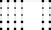
Figure 3: A twin-free graph with a minimal locating-dominating set (depicted as square vertices) whose complement is not a locating-dominating set.

Theorem 4.2.

Let $G$ be a twin-free graph and let $D\subseteq V(G)$ be a minimal dominating set of $G$. Then, $V(G)\setminus D$ is a locating-dominating set of $G$.

Proof.

Let $D$ be a minimal dominating set of $G$. By Theorem 4.1, we only need to prove that $V(G)\setminus D$ is a distinguishing set of $G$. Thus, we shall show that, for every $x,y\in D$, there is a vertex $u\in V(G)\setminus D$ distinguishing $\{x,y\}$. Indeed, it is proved in [39] that $D$ is a minimal dominating set if and only if each vertex $x\in D$ satisfies that either $N(x)\subseteq V(G)\setminus D$ or $N(u)\cap D=\{x\}$ for some $u\in V(G)\setminus D$. Hence, if $N(x),N(y)\subseteq V(G)\setminus D$ then $\{x,y\}$ is distinguished by some $u\in V(G)\setminus D$ since $G$ is twin-free. Otherwise, we can assume without loss of generality that $N(u)\cap D=\{x\}$ for some $u\in V(G)\setminus D$ and so $\{x,y\}$ is distinguished by $u$. Therefore, $V(G)\setminus D$ is a locating-dominating set of $G$, as claimed. ∎

Now, we show a series of consequences of this last result which relate $\lambda(G)$ to well-known graph parameters when $G$ is twin-free. The upper domination number $\Gamma(G)$ of a graph $G$ is the maximum cardinality of a minimal dominating set of $G$. This is a heavily studied invariant which has been related to other well-known parameters in the area of domination (see [30] for multiple examples). With the same spirit, the following consequence of Theorem 4.2 relates the upper domination number to the locating-domination number of a twin-free graph, and supports the validity of Conjecture 2.

Corollary 4.3.

Let $G$ be a twin-free graph. Then,

$$\lambda(G)\leq n-\max{\{\Gamma(G),\Gamma(\overline{G})-1\}}.$$

In particular, $\lambda(G)\leq\frac{n}{2}$ when either $\Gamma(G)\geq\frac{n}{2}$ or $\Gamma(\overline{G})\geq\frac{n}{2}+1$.

Proof.

We deduce from Theorem 4.2 that $\lambda(G)\leq n-\Gamma(G)$ for every twin-free graph $G$. Also, Theorem 7 of [34] shows that $|\lambda(G)-\lambda(\overline{G})|\leq 1$ and so $\lambda(G)\leq\lambda(\overline{G})+1\leq n-\Gamma(\overline{G})+1$ since $\overline{G}$ is also twin-free. Therefore, $\lambda(G)\leq\min\{n-\Gamma(G),n-\Gamma(\overline{G})+1\}$, which is the expected bound. ∎

Recall that the independence number $\alpha(G)$ and the clique number $\omega(G)$ are the maximum cardinalities of an independent set and a complete subgraph of $G$, respectively. The following result relates these two classical parameters to $\lambda(G)$ when $G$ is twin-free, and gives another sufficient condition for $G$ to have $\lambda(G)\leq\frac{n}{2}$.

Corollary 4.4.

Let $G$ be a twin-free graph. Then,

$$\lambda(G)\leq n-\max\{\alpha(G),\omega(G)-1\}.$$

In particular, $\lambda(G)\leq\frac{n}{2}$ when either $\alpha(G)\geq\frac{n}{2}$ or $\omega(G)\geq\frac{n}{2}+1$.

Proof.

Observe first that every independent set $I$ of order $\alpha(G)$ is a minimal dominating set of $G$. Indeed, $I$ is a dominating set since every $x\in V(G)\setminus I$ has a neighbor in $I$ (otherwise $I$ is not an independent set of maximum order) and it is minimal since $N(u)\subseteq V(G)\setminus I$ for every $u\in I$. Hence, $\alpha(G)\leq\Gamma(G)$, and so $\omega(G)=\alpha(\overline{G})\leq\Gamma(\overline{G})$. Thus, combining these inequalities with Corollary 4.3 leads us to the bound since $G$ is twin-free and so is $\overline{G}$. ∎

The chromatic number of $G$, denoted by $\chi(G)$, is the smallest number of classes needed to partition $V(G)$ so that no two adjacent vertices belong to the same class. A classical result in graph theory establishes that $\chi(G)\leq\frac{n+\omega(G)}{2}$ (see for instance [14]). Applying this to $G$ and $\overline{G}$, we can easily deduce from Corollary 4.4 the following bound on $\lambda(G)$ in terms of $\chi(G)$ and $\chi(\overline{G})$ which in particular supports Conjecture 2.

Corollary 4.5.

Let $G$ be a twin-free graph. Then,

$$\lambda(G)\leq 2n-\max\{2\chi(G),2\chi(\overline{G})-1\}.$$

Consequently, $\lambda(G)\leq\frac{n}{2}$ when either $\chi(G)\geq\frac{3}{4}n$ or $\chi(\overline{G})\geq\frac{3}{4}n+\frac{1}{2}$.

Erdős and Szekeres [21] proved that every graph of order $n$ contains either a complete subgraph or an independent set of cardinality at least $\lceil\frac{\log_{2}n}{2}\rceil$. On account of this result and Corollary 4.4, we obtain our first upper bound on $\lambda_{|_{\mathcal{C}^{*}}}(n)$, and consequently on $(\dim-\operatorname{Det})(n)$ and $(\lambda-\operatorname{Det})(n)$ (by Theorem 3.6). Thus, the following corollary improves significatively the bound $(\dim-\operatorname{Det})(n)\leq n-2$ due to Cáceres et al. [8] (see Proposition 1.1 above).

Corollary 4.6.

For every $n\geq 4$,

$$(\dim-\operatorname{Det})(n)\leq(\lambda-\operatorname{Det})(n)\leq\lambda_{|_{\mathcal{C}^{*}}}(n)\leq n-\lceil\frac{\log_{2}n}{2}\rceil+1.$$

5 A greedy algorithm for finding distinguishing sets and determining sets of twin-free graphs

Babai [3] defined distinguishing sets because of their usefulness in the graph isomorphism problem. Indeed, by constructing a canonical labeling, he proved that deciding whether a graph $G$ of order $n$ is isomorphic to any other can be done in $o(n^{s+3})$ time whenever $G$ has a distinguishing set of size $s$. Thus, Babai provided the following result on distinguishing sets by means of a probabilistic argument.

Lemma 5.1.

[3] Let $G$ be a graph of order $n$ and let $k$ be such that $|N(x)\Delta N(y)|\geq k$ for any $x,y\in V(G)$. Then, $G$ has a distinguishing set of cardinality at most $\lceil\frac{2n\log n}{k+2}\rceil$ provided $k>4\log n$.

Note that the graphs considered in this last result are twin-free. Thus, we deduce from Lemma 5.1 and Remark 1.2 another result supporting Conjecture 2: a graph $G$ of order $n\geq 32$ satisfies $\lambda(G)\leq\frac{n}{2}$ whenever $|N(x)\Delta N(y)|>4\log n$ for any $x,y\in V(G)$. Similarly, we provide in this section a polynomial time algorithm that produces distinguishing sets of bounded size but having no restriction on the twin-free graph $G$. Hence, we obtain one of the main results of this paper which is an explicit upper bound on $\lambda_{|_{\mathcal{C^{*}}}}(n)$ (see Subsection 5.1). Also, this algorithm produces determining sets of bounded size and so an upper bound on the determining number of a twin-free graph (see Subsection 5.2). To do this, we next provide some notation.

For any set $D\subseteq V(G)$, let us define a relation on $V(G)$ given by $u\sim_{D}v$ if and only if either $u=v$ or $\{u,v\}$ is distinguished by no vertex of $D$. It is easy to check that this is an equivalence relation, and so we denote by $[u]_{D}$ the set of vertices $v\in V(G)$ so that $u\sim_{D}v$. Thus, let $D^{1}=\{u\in V(G)\setminus D:|[u]_{D}|=1\}$ and $D^{>1}=V(G)\setminus(D\cup D^{1})$. Observe that $D,D^{1},D^{>1}$ form a partition of $V(G)$, where any of these sets may be empty. Actually, $D$ is a distinguishing set if and only if $D^{>1}=\emptyset$.

The following greedy algorithm gives a partition of $V(G)$ into three sets so that, combining them properly, one obtains distinguishing sets and determining sets of $G$ of bounded size, as we shall see in Lemmas 5.2 and 5.5.

1

Input: A twin-free graph $G$ and a vertex $u_{0}\in V(G)$.

Output: An appropriate partition of $V(G)$ into three subsets $A,B,C$.

2

3$A\leftarrow\{u_{0}\}$

4 $B\leftarrow A^{1}$

5 $C\leftarrow A^{>1}$

6 while $\exists$ $u,x,y\in C$ such that $[x]_{A}=[y]_{A}$ and $[x]_{A\cup\{u\}}\neq[y]_{A\cup\{u\}}$ do

7      $A\leftarrow A\cup\{u\}$

8       $B\leftarrow A^{1}$

9       $C\leftarrow A^{>1}$

10      

11 end while

return A,B,C

Algorithm 1

5.1 A better upper bound on $\lambda_{|_{\mathcal{C}^{*}}}(n)$

Colbourn et al. [18] showed that the problem of computing the locating-domination number of an arbitrary graph is NP-hard. Hence, when designing polynomial time algorithms for computing this parameter, it is necessary the restriction to specific families of graphs. Indeed, linearity for trees and series-parallel graphs was proved in [18]. Likewise, for a twin-free graph $G$, we next show that Algorithm 1 returns distinguishing sets of bounded size in polynomial time. Further, this gives a bound on $\lambda_{|_{\mathcal{C}^{*}}}(n)$ which improves that given in Corollary 4.6, and consequently the upper bound of Proposition 1.1 by Cáceres et al. [8].

Lemma 5.2.

Let $A,B,C$ be the sets obtained by application of Algorithm 1 to a twin-free graph $G$ and any vertex $u_{0}\in V(G)$. Then, $A\cup B$, $A\cup C$ and $B\cup C$ are distinguishing sets of $G$.

Proof.

Note first that Algorithm 1 returns a partition of $V(G)$ into three subsets $A,B,C$ such that $B=A^{1}$, $C=A^{>1}$ and no pair $\{x,y\}\subseteq C$ with $[x]_{A}=[y]_{A}$ is distinguished by any $u\in C\setminus\{x,y\}$. $G$ is twin-free and so there must be a vertex $u\in V(G)\setminus\{x,y\}$ distinguishing $\{x,y\}$, which implies that $u\in A\cup B$. Hence, $A\cup B$ is a distinguishing set of $G$ since every pair $\{x,y\}\subseteq C$ is distinguished by some $u\in B$ whenever $[x]_{A}=[y]_{A}$ (otherwise $[x]_{A}\neq[y]_{A}$ and so $\{x,y\}$ is distinguished by some $u\in A$). Also, $A\cup C$ is a distinguishing set since every $x\in V(G)\setminus(A\cup C)=B$ is uniquely determined by $A\subseteq A\cup C$. Finally, to prove that $B\cup C$ is a distinguishing set, let $x_{1},...,x_{|A|}$ be the elements of $A$ sorted by appearance in Algorithm 1. We shall prove that every pair $\{x_{i},x_{j}\}$ with $i<j$ is distinguished by some vertex of $B\cup C$.

In the $i$-th step of the algorithm, a vertex $u\in C$ is added to $A$ and becomes $x_{i}$ because $u$ distinguishes a pair $\{x,y\}\subseteq C$ such that $[x]_{A}=[y]_{A}$ and so this class is splat into two new classes $[x]_{A\cup\{x_{i}\}}$ and $[y]_{A\cup\{x_{i}\}}$. Thus, any pair $\{\alpha,\beta\}$ with $\alpha\in[x]_{A\cup\{x_{i}\}}$ and $\beta\in[y]_{A\cup\{x_{i}\}}$ is distinguished by $x_{i}$ and non-distinguished by any of $x_{1},...,x_{i-1}$. Moreover, in the following steps, it always remains one such pair $\{\alpha,\beta\}\subseteq B\cup C$. Indeed, when $u$ is sent to $A$, there is another vertex $u^{\prime}\in[u]_{A}$ which either stays in $C$ or goes to $B$ since $C$ is formed by vertices of non-unitary classes. It follows that for every pair $\{x_{j},x_{k}\}$ with $j<k$, there exists a pair $\{\alpha,\beta\}\subseteq B\cup C$ non-distinguished by $x_{j}$ but distinguished by $x_{k}$. Thus, assume without loos of generality that $x_{j}\in N(\alpha)\cap N(\beta)$ and $x_{k}\in N(\alpha)\setminus N(\beta)$ (the remaining cases are analogous). Hence, $\{x_{j},x_{k}\}$ is distinguished by $\beta$, which completes the proof. ∎

The pigeonhole principle ensures that one set among $A,B,C$ has cardinality at least $\lceil\frac{n}{3}\rceil$ and so one of $A\cup B,A\cup C,B\cup C$ has cardinality at most $\lfloor\frac{2}{3}n\rfloor$. Then, by Lemma 5.2 and Remark 1.2, we have the following result.

Theorem 5.3.

Let $G$ be a twin-free graph of order $n\geq 4$. Then, there exists a locating-dominating set of $G$ of cardinality at most $\lfloor\frac{2}{3}n\rfloor+1$ which can be computed in polynomial time. In particular,

$$\lambda_{|_{\mathcal{C}^{*}}}(n)\leq\lfloor\frac{2}{3}n\rfloor+1.$$

The next corollary summarizes some of the main results of this paper, i.e., Theorems 2.2, 3.6 and 5.3. As far as we know, these are the best bounds on the function $(\dim-\operatorname{Det})(n)$.

Corollary 5.4.

For every $n\geq 14$,

$$\lfloor\frac{n}{2}\rfloor-1\leq(\dim-\operatorname{Det})(n)\leq(\lambda-\operatorname{Det})(n)\leq\lambda_{|_{\mathcal{C}^{*}}}(n)\leq\lfloor\frac{2}{3}n\rfloor+1.$$

5.2 An upper bound on $\operatorname{Det}(G)$ for twin-free graphs

Blaha [5] showed that finding a minimum base of a permutation group is NP-hard and provided a greedy algorithm for constructing bases. The same algorithm was given by Gibbons and Laison [27] in the particular case of automorphism groups of graphs: for a graph $G$ of order $n$, the algorithm returns a determining set of size $O(\operatorname{Det}(G)\log\log n)$. Observe that this algorithm does not yield a bound on the determining number of $G$ in terms of $n$. However, we next show that Algorithm 1 gives an explicit upper bound on $\operatorname{Det}(G)$ when $G$ is twin-free by constructing a determining set of bounded size in polynomial time.

Lemma 5.5.

Let $A,B,C$ be the sets obtained by application of Algorithm 1 to a twin-free graph $G$ and any vertex $u_{0}\in V(G)$. Then, $A$ and $B\cup C$ are determining sets of $G$.

Proof.

We have proved in Lemma 5.2 that $B\cup C$ is a distinguishing set of $G$, which implies that it is also a resolving set and so it is a determining set. To prove that $A$ is a determining set of $G$, we first claim that $stab(A)=stab(A\cup\{x\})$ for every $x\in B$. Indeed, $stab(A)\supseteq stab(A\cup\{x\})$, by definition of the stabilizer. Also, note that $N(x)\cap A$ is unique since $B=A^{1}$, and recall that automorphisms preserve adjacencies. Thus, no automorphism fixing every vertex of $A$ can interchange $x$ with any other vertex of $V(G)$. Hence, $stab(A)\subseteq stab(A\cup\{x\})$. Therefore, extending this argument to every vertex of $B$, we obtain that $stab(A)=stab(A\cup B)$. But $A\cup B$ is a distinguishing set by Lemma 5.2 and so it is a determining set, which implies that $stab(A\cup B)=stab(A)=\{id_{G}\}$. It follows that $A$ is a determining set. ∎

Reasoning as in the previous subsection, we have that either $A$ or $B\cup C$ has cardinality at most $\lfloor\frac{n}{2}\rfloor$ and so, by Lemma 5.5, we obtain the following bound.

Theorem 5.6.

Let $G$ be a twin-free graph of order $n\geq 4$. Then, there exists a determining set of $G$ of cardinality at most $\lfloor\frac{n}{2}\rfloor$ which can be computed in polynomial time. In particular,

$$\operatorname{Det}(G)\leq\lfloor\frac{n}{2}\rfloor.$$

Note that, although the graph depicted in Figure 4 does not prove tightness for this last result, this construction shows that we are very close to a tight bound.

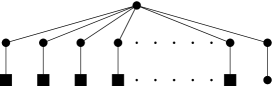
Figure 4: A graph $G$ with a determining set (illustrated with square vertices) of size $\operatorname{Det}(G)=\lfloor\frac{|V(G)|}{2}\rfloor-1$.

6 Useful tools for the problems restricted to graphs without $K_{2,k}$ as subgraph

6.1 $k$-domination

The concept of $k$-dominating set was introduced by Fink and Jacobson [24] as a generalization of classical dominating sets of graphs. There is a wealth of literature about this variety of domination (see [15] and the references given there). Specifically, the $k$-domination number $\gamma_{k}(G)$ has been related to other graph parameters such as the path covering number [19], the order and the minimum degree [23] and the $j$-dependence number [24]. In this subsection, we establish a relationship between $\gamma_{k}(G)$ and $\lambda(G)$ when $G$ does not contain $K_{2,k}$ as a subgraph. To do this, we require Lemma 6.1 below which, in addition, is a key result in the following subsection for computing the restriction of $(\lambda-\operatorname{Det})(n)$ to this class of graphs when $k=2$.

Given a set $D\subseteq V(G)$, a vertex $x\in V(G)\setminus D$ and a positive integer $k$, we say that $x$ is $k$-dominated by $D$ if $|N(x)\cap D|\geq k$, and $D$ is a $k$-dominating set of $G$ if every vertex of $V(G)\setminus D$ is $k$-dominated by $D$. The $k$-domination number of $G$, denoted by $\gamma_{k}(G)$, is the minimum cardinality of a $k$-dominating set of $G$. It is straightforward that $\gamma_{1}(G)=\gamma(G)$ and $\gamma_{k}(G)\leq\gamma_{\ell}(G)$ for every $k,\ell$ with $1\leq k\leq\ell$.

Let $\mathcal{K}_{2,k}$ denote the class of graphs not containing $K_{2,k}$ as a (not necessarily induced) subgraph. The following lemma contains the main idea for proving Proposition 6.2.

Lemma 6.1.

Let $G\in\mathcal{K}_{2,k}$, $D\subseteq V(G)$ and $x\in V(G)\setminus D$. If $x$ is $k$-dominated by $D$ then, for every $y\in V(G)\setminus D$, the pair $\{x,y\}$ is distinguished by some vertex of $D$.

Proof.

Let $y\in V(G)\setminus D$ and $A\subseteq N(x)\cap D$ such that $|A|=k$. Clearly, some vertex of $A$ distinguishes $\{x,y\}$ since otherwise $A\subseteq N(y)$ and so the induced subgraph by $A\cup\{x,y\}$ contains a copy of $K_{2,k}$, which is impossible. ∎

Hence, a $k$-dominating set of $G$ is a locating-dominating set whenever $G\in\mathcal{K}_{2,k}$ but the converse is not true in general, as shown in Figure 5. Further, it was proved in [16] that $\gamma_{k}(G)\leq\frac{k}{k+1}n$ for any graph $G$ such that $k\leq\delta(G)$. Thus, we have the following result.

Proposition 6.2.

For every $G\in\mathcal{K}_{2,k}$, it holds that

$$\gamma(G)\leq\lambda(G)\leq\gamma_{k}(G).$$

In particular, $\lambda(G)\leq\frac{k}{k+1}n$ whenever $\delta(G)\geq k$.

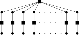
Figure 5: A graph in $\mathcal{K}_{2,2}$ with a locating-dominating set (depicted as square vertices) which is not a 2-dominating set.

Let us denote by $\mathcal{C}_{4}$ the class $\mathcal{K}_{2,2}$, i.e., the set of graphs not having $C_{4}=K_{2,2}$ as a subgraph. The following corollary is a consequence of Proposition 6.2 when $k=2$, and gives essentially the same bound as the one provided by Corollary 5.4. However, this bound will be improved in the following subsection (see Theorem 6.7).

Corollary 6.3.

Let $G\in\mathcal{C}_{4}$ be such that $\delta(G)\geq 2$. Then, $\lambda(G)-\operatorname{Det}(G)\leq\frac{2}{3}n$.

6.2 Matchings

The matching number $\alpha^{\prime}(G)$ has been related to many domination parameters (see for instance [6, 17, 32, 33]). As an example, Henning et al. [32] related the matching number to the total domination number $\gamma_{t}(G)$, i.e., the minimum size of a set of vertices dominating every vertex of $G$. Concretely, they proved that $\gamma_{t}(G)\leq\alpha^{\prime}(G)$ whenever $G$ is either a claw-free graph or a $k$-regular graph with $k\geq 3$. In the same vein, we obtain a similar relationship between $\alpha^{\prime}(G)$ and $\lambda(G)$ when $G$ is a twin-free graph in $\mathcal{C}_{4}$ (see Proposition 6.6). Besides its independent interest, we apply this relation to study the functions $({\rm dim}-{\rm Det})_{|_{\mathcal{C}_{4}}}(n)$ and $(\lambda-{\rm Det})_{|_{\mathcal{C}_{4}}}(n)$ (see Theorems 6.7 and 6.8).

A matching $M$ in a graph $G$ is a subset of pairwise disjoint edges of $G$, and the matching number of $G$, written as $\alpha^{\prime}(G)$, is the cardinality of a maximum matching in $G$. We denote by $\overline{M}$ the set of vertices of $G$ in no edge of $M$. Observe that $\overline{M}$ is an independent set when $M$ is maximum (otherwise there is an edge $e=\{x,y\}$ with $x,y\in\overline{M}$ and so the matching $M^{\prime}=M\cup\{e\}$ has more edges than $M$, which is impossible). The following is a technical lemma that captures all possible situations for the edges of a maximum matching (see Figure 6).

Lemma 6.4.

Let $M$ be a maximum matching in $G$. Then, for every $\{u,v\}\in M$, exactly one of the following cases holds:

1. $N(u)\cap\overline{M}=N(v)\cap\overline{M}=\emptyset$.

2. Either $N(u)\cap\overline{M}\neq\emptyset$ or $N(v)\cap\overline{M}\neq\emptyset$, but not both.

3. $N(u)\cap\overline{M}=N(v)\cap\overline{M}=\{x\}$ for some $x\in\overline{M}$.

Proof.

Let $M$ be a maximum matching in $G$. It is enough to prove that there is no edge $e=\{u,v\}$ in $M$ and vertices $x,y\in\overline{M}$ such that $x\in N(u)$ and $y\in N(v)$. Indeed, $(M\setminus\{e\})\cup\{\{u,x\},\{v,y\}\}$ would be a matching in $G$ with more edges than $M$, which is impossible. ∎

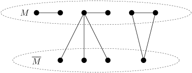
Figure 6: The three cases for the edges of a maximum matching $M$ provided by Lemma 6.4.

For every matching $M$ in $G$, let us consider the set

$$U_{M}=\{x\in\overline{M}:N(x)\subseteq e\quad for\quad some\quad e\in M\}.$$

Note that, when $M$ is maximum, $U_{M}$ is formed by all vertices $x\in\overline{M}$ such that $\delta(x)=1$ or $N(x)=e$ for some $e\in M$. We next show another technical result which is required in the proof of Proposition 6.6.

Lemma 6.5.

Let $G$ be a twin-free graph. Then, there exists a maximum matching $M$ such that $U_{M}=\emptyset$ which can be computed in polynomial time.

Proof.

Let $M$ be a maximum matching in $G$. Observe first that no two vertices $x,y\in U_{M}$ satisfy $N(x),N(y)\subseteq e$ for any $e\in M$ (otherwise Lemma 6.4 yields $\delta(x)=\delta(y)=1$ and $N(x)=N(y)$, which contradicts the fact that $G$ is twin-free).

If $U_{M}\neq\emptyset$ then let $x\in U_{M}$ and $e=\{u,v\}$ in $M$ with $N(x)\subseteq e$. Thus, assuming that $u\in N(x)$, we claim that $M^{\prime}=(M\setminus\{e\})\cup\{\{u,x\}\}$ is a maximum matching in $G$ such that $U_{M^{\prime}}=U_{M}\setminus\{x\}$. Clearly, $U_{M}\setminus\{x\}\subseteq U_{M^{\prime}}$. Indeed, for every $y\in U_{M}\setminus\{x\}\subseteq\overline{M}^{\prime}$ there exists an edge $f\in M$ such that $N(y)\subseteq f$. As remarked above, $f\neq e$ since $x\neq y$, which implies that $f\in(M\setminus e)\subseteq M^{\prime}$ and so $y\in U_{M^{\prime}}$.

We now prove that $U_{M^{\prime}}\subseteq U_{M}\setminus\{x\}$. Let $y\in U_{M^{\prime}}$ such that $N(y)\subseteq f$ for some $f\in M^{\prime}$. If $f\in M\setminus\{e\}$ then $y\in U_{M}\setminus\{x\}$ (note that $y\neq v$ since $v\in N(u)$ and so there is no $f\in M\setminus\{e\}$ with $N(v)\subseteq f$). Otherwise, $f=\{u,x\}$. If $y\neq v$ then $y\notin N(x)$ since $\overline{M}$ is an independent set, and then $N(y)=\{u\}$. However, $N(x)\subseteq e$ and so Lemma 6.4 ensures that $N(x)=N(y)=\{u\}$; a contradiction since $G$ is twin-free. Therefore, $y=v$ and we easily get either $N(v)=N(x)=\{u\}$ or $N[v]=N[x]=\{u,v,x\}$; again a contradiction. Thus, we have proved that $U_{M^{\prime}}=U_{M}\setminus\{x\}$ and iterating this process gives a maximum matching $M^{*}$ with $U_{M^{*}}=\emptyset$. Observe that $M$ can be found in polynomial time [20] and $M^{*}$ is easily obtained from $M$ also in polynomial time. Hence, we can compute $M^{*}$ in polynomial time, as claimed.

∎

We now reach one of the main results of this section which relates $\alpha^{\prime}(G)$ and $\lambda(G)$ when $G$ is a twin-free graph in $\mathcal{C}_{4}$.

Proposition 6.6.

Let $G\in\mathcal{C}_{4}$ be a twin-free graph of order $n\geq 4$. Then, there is a locating-dominating set of $G$ of cardinality $\alpha^{\prime}(G)$ which can be computed in polynomial time, and consequently

$$\lambda(G)\leq\alpha^{\prime}(G).$$

In particular, $\lambda(G)\leq\frac{n}{2}$.

Proof.

Let $M$ be a maximum matching in $G$ satisfying that $U_{M}=\emptyset$, which exists by Lemma 6.5. We consider a partition $V(G)=V_{1}\cup V_{2}\cup\overline{M}$ such that $e\cap V_{1}$ and $e\cap V_{2}$ are non-empty for every $e\in M$, i.e., $V_{1}$ and $V_{2}$ contain the endpoints of every $e\in M$, respectively. By Lemma 6.4, for every $e=\{u,v\}$ in $M$ and $x\in\overline{M}$ with $N(x)\cap e=\{u\}$, we can assume without loss of generality that $u\in V_{1}$. This means that every $e=\{u,v\}$ in $M$ so that $N(u)\cap\overline{M}\neq\emptyset$ and $N(v)\cap M=\emptyset$ satisfies $u\in V_{1}$. Thus, we shall prove that $V_{1}$ is a locating-dominating set of $G$.

It is easy to check that $V_{1}$ is a dominating set of $G$ by construction of $V_{1}$ and $V_{2}$. Furthermore, every $x\in\overline{M}$ is 2-dominated by $V_{1}$. Indeed, $N(x)$ intersects at least two different edges of $M$ since $U_{M}=\emptyset$. Thus, let $u,u^{\prime}\in N(x)$ with $\{u,v\},\{u^{\prime},v^{\prime}\}\in M$ for some $v,v^{\prime}\in V(G)$. Since we can suppose $u,u^{\prime}\in V_{1}$, we have that $x$ is 2-dominated by $\{u,u^{\prime}\}\subseteq V_{1}$.

To prove that $V_{1}$ is a distinguishing set of $G$, we claim that every pair $\{x,y\}\subseteq V_{2}\cup\overline{M}$ is distinguished by some $u\in V_{1}$. By Lemma 6.1, we can assume that $x,y\in V_{2}$ since every vertex of $\overline{M}$ is 2-dominated by $V_{1}$ and $G\in\mathcal{C}_{4}$. Thus, let $u,u^{\prime}\in V_{1}$ such that $\{u,x\},\{u^{\prime},y\}\in M$. Hence, one of $u$ or $u^{\prime}$ resolves $\{x,y\}$ since otherwise $u\in N(y)$ and $u^{\prime}\in N(x)$, which produces the cycle $(u,x,u^{\prime},y)$; a contradiction with $G\in\mathcal{C}_{4}$. Therefore, we have proved that $V_{1}$ is a locating-dominating set of $G$ (obtained in polynomial time by Lemma 6.5) and so $\lambda(G)\leq|V_{1}|=\alpha^{\prime}(G)\leq\frac{n}{2}$, as claimed. ∎

As an application of this last result, we next compute the exact value of $(\lambda-\operatorname{Det})_{|_{{\mathcal{C}_{4}}}}(n)$ and give bounds on $(\dim-\operatorname{Det})_{|_{{\mathcal{C}_{4}}}}(n)$, supporting again the validity of Conjecture 2.

Theorem 6.7.

For every $n\geq 14$, it holds that

$$(\lambda-\operatorname{Det})_{|_{{\mathcal{C}_{4}}}}(n)=\lfloor\frac{n}{2}\rfloor.$$

Proof.

Mimicking the proof of Theorem 2.2 on $(\lambda-\operatorname{Det})(n)$ yields $(\lambda-\operatorname{Det})_{|_{{\mathcal{C}_{4}}}}(n)\geq\lfloor\frac{n}{2}\rfloor$ since the graphs considered belong to $\mathcal{C}_{4}$. To prove the reverse inequality, it suffices to show that every graph $G\in\mathcal{C}_{4}$ of order $n$ satisfies $\lambda(G)-\operatorname{Det}(G)\leq\frac{n}{2}$. Indeed, let us assume first that $G^{*}\not\cong K_{2}$ (otherwise $\lambda(G)-\operatorname{Det}(G)\leq 1<\frac{n}{2}$ by Lemma 3.3). Thus, the graph $\widetilde{G}$ described in Section 3 satisfies $\lambda(G)-\operatorname{Det}(G)\leq\lambda(\widetilde{G})$, by Proposition 3.5. Also, Lemma 3.4 guarantees that $\widetilde{G}$ is twin-free and has order $\widetilde{n}\leq n$. Hence, Proposition 6.6 gives $\lambda(\widetilde{G})\leq\frac{\widetilde{n}}{2}\leq\frac{n}{2}$ since it is easily seen that $\widetilde{G}\in\mathcal{C}_{4}$. Therefore, we have proved that $\lambda(G)-\operatorname{Det}(G)\leq\lambda(\widetilde{G})\leq\frac{n}{2}$, as required. ∎

Theorem 6.8.

For every $n\geq 49$, it holds that

$$\lfloor\frac{2}{7}n\rfloor\leq(\dim-\operatorname{Det})_{|_{{\mathcal{C}_{4}}}}(n)\leq\lfloor\frac{n}{2}\rfloor.$$

Proof.

The upper bound follows immediately from Expression (1) and Theorem 6.7. For the lower bound, we shall construct a graph $G$ of order $n$ not containing $C_{4}$ as a subgraph such that $(\dim-\operatorname{Det})(G)=\lfloor\frac{2}{7}n\rfloor$. Indeed, let $n=7q+s$ for some integers $q,s$ with $q\geq 7$ and $0\leq s<7$. The graph $T_{q,0}$ is given by attaching a copy of $T_{6}$ to every vertex of $T_{q-1}$ as shown in Figure 7(a) (recall that the tree $T_{r}$ is described in Section 2). If $s\in\{1,2,3\}$ then $T_{q,s}$ is obtained from $T_{q,0}$ by replacing the edge $\{u_{1},u_{2}\}$ by a path of length $s+1$ (see Figure 7(b)). Otherwise, $s\in\{4,5,6\}$ and $T_{q,s}$ comes from $T_{q,0}$ by attaching a path of length $s$ to $u_{1}$ (see Figure 7(c)). It is clear that $aut(T_{q,s})=id_{T_{q,s}}$, which implies that $\operatorname{Det}(T_{q,s})=0$. Further, the metric bases illustrated in Figure 7 (see Section 7 for more information on metric dimension of trees) show that

$$\dim(T_{q,s})=\left\{\begin{array}[]{lcc}2q&if&s\in\{0,1,2,3\}\\ \\ 2q+1&if&s\in\{4,5,6\}\end{array}\right.$$

But $n=|V(T_{q,s})|$ and so $\dim(T_{q,s})=\lfloor\frac{2}{7}n\rfloor$. Therefore, setting $G\cong T_{q,s}$ yields the expected bound.

∎

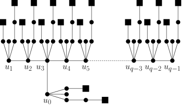
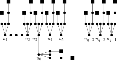
(a)		(b)

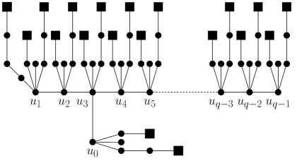
(c)

Figure 7: Metric bases (depicted as square vertices) of the graphs (a) $T_{q,0}$, (b) $T_{q,3}$ and (c) $T_{q,5}$.

7 Computing the functions restricted to trees

Cáceres et al. [8] started the study of the difference between the determining number and the metric dimension of trees when trying to answer the question raised by Boutin [7]. Actually, they constructed a family of trees where this difference is $\Omega(\sqrt{n})$. This section completely solves this particular problem showing that the trees $T_{q,s}$ described in the preceding section have the maximum value of $\dim(G)-\operatorname{Det}(G)$ in the class of trees (see Theorem 7.4). Moreover, we compute the maximum value of $\lambda(G)-\operatorname{Det}(G)$ restricted to trees (see Theorem 7.5).

Some of the terminology that we adopt in this section can be found in [11]. Given a tree $T$, a vertex of degree at least 3 is called a major vertex of $T$. A pendant vertex $\ell$ is a terminal vertex of a major vertex $u$ if the major vertex closest to $\ell$ in $T$ is $u$. The terminal degree of a major vertex $u$, denoted by $ter(u)$, is the number of terminal vertices of $u$. A major vertex $u$ is an exterior major vertex of $T$ if it has positive terminal degree in $T$. The set of exterior major vertices of $T$ is denoted by $Ex(T)$.

The metric dimension of any tree is well-known (see for instance [11, 28, 37, 42]) and its formula is exhibited next.

Proposition 7.1.

[37] If $T$ is a tree that is not a path, then

$$\dim(T)=\sum_{u\in Ex(T)}(ter(u)-1).$$

First, we provide two technical lemmas which aid in proving Theorem 7.4. We denote by $ter^{\prime}(u)$ the number of different distances between $u$ and any of its terminal vertices. For every $u\in Ex(T)$, we write $N_{u}$ for the set of vertices in some $u$-$\ell$ shortest path, where $\ell$ is a terminal vertex of $u$; the cardinality of $N_{u}$ is denoted by $n_{u}$.

Lemma 7.2.

Let $T$ be a tree and $u\in Ex(T)$. Then, $ter^{\prime}(u)\leq\frac{2}{7}n_{u}+1$.

Proof.

Let $d_{1},d_{2},...,d_{ter^{\prime}(u)}$ with $d_{1}<d_{2}<...<d_{ter^{\prime}(u)}$ be the different distances between $u$ and any of its terminal vertices. Thus, $\displaystyle n_{u}\geq(\sum_{i=1}^{ter^{\prime}(u)}d_{i})+1$, and consequently

$$n_{u}\geq(\sum_{i=1}^{ter^{\prime}(u)}i)+1=\frac{ter^{\prime}(u)(ter^{\prime}(u)+1)}{2}+1.$$

Hence, an easy computation shows that $ter^{\prime}(u)\leq\frac{\sqrt{8n_{u}-7}-1}{2}\leq\frac{2}{7}n_{u}+1$. ∎

Lemma 7.3.

Let $T$ be a tree that is not a path. Then,

$$\operatorname{Det}(T)\geq\sum_{u\in Ex(T)}(ter(u)-ter^{\prime}(u)).$$

Proof.

Let $S$ be a minimum determining set of $T$. As shown in [22], we can assume that $S$ is only formed by pendant vertices. Consider a vertex $u\in Ex(T)$ and two of its terminal vertices, say $\ell$ and $\ell^{\prime}$, such that $d(u,\ell)=d(u,\ell^{\prime})$. Clearly, either $\ell$ or $\ell^{\prime}$ belongs to $S$ (otherwise there is an automorphism interchanging the $u-\ell$ path and the $u-\ell^{\prime}$ path, and fixing the remaining vertices of $V(T)$ but $S$ is a determining set; a contradiction). Therefore, at least $ter(u)-ter^{\prime}(u)$ vertices of $N_{u}$ are in $S$, and extending this argument to $Ex(T)$ yields the bound. ∎

We now achieve one of the main results of this section which provides the exact value of the function $(\dim-\operatorname{Det})_{|_{\mathcal{T}}}(n)$, where $\mathcal{T}$ denotes the family of trees.

Theorem 7.4.

For every $n\geq 49$, it holds that

$$(\dim-\operatorname{Det})_{|_{\mathcal{T}}}(n)=\lfloor\frac{2}{7}n\rfloor.$$

Proof.

We first prove that $(\dim-\operatorname{Det})(T)\leq\lfloor\frac{2}{7}n\rfloor$ for any tree $T$ of order $n$. Thus, we can assume that $T$ is not a path since it is clear that $\dim(P_{n})-\operatorname{Det}(P_{n})=1-1=0$ for every $n\geq 2$. By Proposition 7.1,

$$\begin{array}[]{ccl}\dim(T)&=&\displaystyle\sum_{u\in Ex(T)}(ter(u)-1)\\ &=&\displaystyle\sum_{u\in Ex(T)}(ter(u)-ter^{\prime}(u))+\sum_{u\in Ex(T)}(ter^{\prime}(u)-1).\end{array}$$

Hence, according to Lemma 7.3, we get

$$\dim(T)-\operatorname{Det}(T)\leq\sum_{u\in Ex(T)}(ter^{\prime}(u)-1)\leq\frac{2}{7}n,$$

the last inequality being a consequence of Lemma 7.2. This shows that $(\dim-\operatorname{Det})_{|_{\mathcal{T}}}(n)\leq\lfloor\frac{2}{7}n\rfloor$ and equality is given by the graphs $T_{q,s}$ constructed in the proof of Theorem 6.8, which are trees. ∎

We want to stress that this last result ensures that trees are not the appropriate family of graphs for disproving Conjecture 1 and shows how far is the bound $\Omega(\sqrt{n})$ due to Cáceres et al. [8].

Since trees do not contain $C_{4}$ as a subgraph, i.e., $\mathcal{T}\subset\mathcal{C}_{4}$, then $(\lambda-\operatorname{Det})_{|_{\mathcal{T}}}(n)\leq(\lambda-\operatorname{Det})_{|_{\mathcal{C}_{4}}}(n)=\lfloor\frac{n}{2}\rfloor$, by Theorem 6.7. Further, the graphs in the proof of Theorem 2.2 are trees and so we get the following result.

Theorem 7.5.

For every $n\geq 14$, it holds that

$$(\lambda-\operatorname{Det})_{|_{\mathcal{T}}}(n)=\lfloor\frac{n}{2}\rfloor.$$

8 Concluding remarks and open questions

In this paper, we have studied the function $(\dim-\operatorname{Det})(n)$ for which we have developed an independent study on $(\lambda-\operatorname{Det})(n)$ and $\lambda_{|_{\mathcal{C}^{*}}}(n)$. Thus, we provide lower and upper bounds on these functions which in particular improve those given by Cáceres et al. [8] for $(\dim-\operatorname{Det})(n)$. To do this, we construct two appropriate families of graphs for improving the lower bound. For the upper bound, we develop a technique which uses locating-dominating sets as a main tool. Indeed, we show that $(\dim-\operatorname{Det})(n)$ and $(\lambda-\operatorname{Det})(n)$ are bounded above by the function $\lambda_{|_{\mathcal{C}^{*}}}(n)$. To obtain bounds on this function, we first provide a variant of a well-known theorem by Ore [39] which implies a number of consequences between the locating-domination number and other graph parameters. One of these consequences yields a first upper bound on $\lambda_{|_{\mathcal{C}^{*}}}(n)$ by means of a classical result due to Erdős and Szekeres [21].

The second upper bound on $\lambda_{|_{\mathcal{C}^{*}}}(n)$ comes from the designing of a polynomial time algorithm that produces both distinguishing sets and determining sets of twin-free graphs. Thus, we also obtain a bound on the determining number of a twin-free graph.

Finally, we restrict ourselves to graphs not having $K_{2,k}$ as a subgraph, thus relating the locating-domination number to the $k$-domination number and the matching number. These relations produce bounds and exact values of the restrictions of $(\dim-\operatorname{Det})(n)$ and $(\lambda-\operatorname{Det})(n)$ to the graphs without $C_{4}$ as a subgraph and the class of trees. Specifically, we solve the problem first considered by Cáceres et al. [8] about the difference between the determining number and the metric dimension of a tree.

It would be interesting to settle Conjectures 1 and 2, which predict the exact values of the functions $(\dim-\operatorname{Det})(n)$, $(\lambda-\operatorname{Det})(n)$ and $\lambda_{|_{\mathcal{C}^{*}}}(n)$ . Also, it remains open the computation of the function $({\rm dim}-{\rm Det})_{|_{\mathcal{C}_{4}}}(n)$. Further, it would be also of interest to find particular families of graphs where the restrictions of $(\dim-\operatorname{Det})(n)$ and $(\lambda-\operatorname{Det})(n)$ may be computed. Finally, the maximum value of the difference between the metric dimension and the locating-domination number is still unknown and a study on this function may be proposed.

References

- [1] D. Auger. Induced paths in twin-free graphs. Electron. J. Combin., 15(1):Research Paper 17, 7, 2008.
- [2] D. Auger, I. Charon, I. Honkala, O. Hudry, and A. Lobstein. Edge number, minimum degree, maximum independent set, radius and diameter in twin-free graphs. Adv. Math. Commun., 3(1):97–114, 2009.
- [3] L. Babai. On the complexity of canonical labeling of strongly regular graphs. SIAM J. Comput., 9(1):212–216, 1980.
- [4] R. F. Bailey and P. J. Cameron. Base size, metric dimension and other invariants of groups and graphs. Bull. Lond. Math. Soc., 43(2):209–242, 2011.
- [5] K. D. Blaha. Minimum bases for permutation groups: the greedy approximation. J. Algorithms, 13(2):297–306, 1992.
- [6] B. Bollobás and E. J. Cockayne. Graph-theoretic parameters concerning domination, independence, and irredundance. J. Graph Theory, 3(3):241–249, 1979.
- [7] D. L. Boutin. Identifying graph automorphisms using determining sets. Electron. J. Combin., 13(1):Research Paper 78, 12, 2006.
- [8] J. Cáceres, D. Garijo, M. L. Puertas, and C. Seara. On the determining number and the metric dimension of graphs. Electron. J. Combin., 17(1):Research Paper 63, 20, 2010.
- [9] G. G. Chappell, J. Gimbel, and C. Hartman. Bounds on the metric and partition dimensions of a graph. Ars Combin., 88:349–366, 2008.
- [10] I. Charon, I. Honkala, O. Hudry, and A. Lobstein. Structural properties of twin-free graphs. Electron. J. Combin., 14(1):Research Paper 16, 15, 2007.
- [11] G. Chartrand, L. Eroh, M. A. Johnson, and O. R. Oellermann. Resolvability in graphs and the metric dimension of a graph. Discrete Appl. Math., 105(1-3):99–113, 2000.
- [12] G. Chartrand, C. Poisson, and P. Zhang. Resolvability and the upper dimension of graphs. Comput. Math. Appl., 39(12):19–28, 2000.
- [13] G. Chartrand and P. Zhang. On the chromatic dimension of a graph. In Proceedings of the Thirty-first Southeastern International Conference on Combinatorics, Graph Theory and Computing (Boca Raton, FL, 2000), volume 145, pages 97–108, 2000.
- [14] G. Chartrand and P. Zhang. Chromatic graph theory. Discrete Mathematics and its Applications (Boca Raton). CRC Press, Boca Raton, FL, 2009.
- [15] M. Chellali, O. Favaron, A. Hansberg, and L. Volkmann. -domination and -independence in graphs: a survey. Graphs Combin., 28(1):1–55, 2012.
- [16] E. J. Cockayne, B. Gamble, and B. Shepherd. An upper bound for the -domination number of a graph. J. Graph Theory, 9(4):533–534, 1985.
- [17] E. J. Cockayne, S. T. Hedetniemi, and P. J. Slater. Matchings and transversals in hypergraphs, domination and independence in trees. J. Combin. Theory Ser. B, 26(1):78–80, 1979.
- [18] C. J. Colbourn, P. J. Slater, and L. K. Stewart. Locating-dominating sets in series parallel networks. Congr. Numer., 56:135–162, 1987. Sixteenth Manitoba conference on numerical mathematics and computing (Winnipeg, Man., 1986).
- [19] E. DeLaViña, C. E. Larson, R. Pepper, and B. Waller. Graffiti.pc on the 2-domination number of a graph. In Proceedings of the Forty-First Southeastern International Conference on Combinatorics, Graph Theory and Computing, volume 203, pages 15–32, 2010.
- [20] J. Edmonds. Paths, trees, and flowers. Canadian Journal of Mathematics, 17:449–467, 1965.
- [21] P. Erdős and G. Szekeres. A combinatorial problem in geometry. Compositio Math., 2:463–470, 1935.
- [22] D. Erwin and F. Harary. Destroying automorphisms by fixing nodes. Discrete Math., 306(24):3244–3252, 2006.
- [23] O. Favaron, A. Hansberg, and L. Volkmann. On -domination and minimum degree in graphs. J. Graph Theory, 57(1):33–40, 2008.
- [24] J. F. Fink and M. S. Jacobson. -domination in graphs. In Graph theory with applications to algorithms and computer science (Kalamazoo, Mich., 1984), Wiley-Intersci. Publ., pages 283–300. Wiley, New York, 1985.
- [25] F. Foucaud, S. Gravier, R. Naserasr, A. Parreau, and P. Valicov. Identifying codes in line graphs. J. Graph Theory, 73(4):425–448, 2013.
- [26] D. Garijo, A. González, and A. Márquez. On the metric dimension, the upper dimension and the resolving number of graphs. Discrete Appl. Math., 161(10-11):1440–1447, 2013.
- [27] C. R. Gibbons and J. D. Laison. Fixing numbers of graphs and groups. Electron. J. Combin., 16(1):Research Paper 39, 13, 2009.
- [28] F. Harary and R. A. Melter. On the metric dimension of a graph. Ars Combinatoria, 2:191–195, 1976.
- [29] H. Hatami, J. Hladký, D. Král’, S. Norine, and A. Razborov. On the number of pentagons in triangle-free graphs. J. Combin. Theory Ser. A, 120(3):722–732, 2013.
- [30] T. W. Haynes, S. T. Hedetniemi, and P. J. Slater. Fundamentals of domination in graphs, volume 208 of Monographs and Textbooks in Pure and Applied Mathematics. Marcel Dekker Inc., New York, 1998.
- [31] P. Heggernes, D. Meister, and C. Papadopoulos. Graphs of linear clique-width at most 3. In Theory and applications of models of computation, volume 4978 of Lecture Notes in Comput. Sci., pages 330–341. Springer, Berlin, 2008.
- [32] M. A. Henning, L. Kang, E. Shan, and A. Yeo. On matching and total domination in graphs. Discrete Math., 308(11):2313–2318, 2008.
- [33] M. A. Henning and A. Yeo. Total domination and matching numbers in graphs with all vertices in triangles. Discrete Math., 313(2):174–181, 2013.
- [34] C. Hernando, M. Mora, and I. M. Pelayo. Nordhaus-Gaddum bounds for locating domination. European J. Combin., 36:1–6, 2014.
- [35] C. Hernando, M. Mora, I. M. Pelayo, C. Seara, and D. R. Wood. Extremal graph theory for metric dimension and diameter. Electron. J. Combin., 17(1):Research Paper 30, 28, 2010.
- [36] M. Jannesari and B. Omoomi. On randomly -dimensional graphs. Appl. Math. Lett., 24(10):1625–1629, 2011.
- [37] S. Khuller, B. Raghavachari, and A. Rosenfeld. Landmarks in graphs. Discrete Appl. Math., 70(3):217–229, 1996.
- [38] A. Kotlov and L. Lovász. The rank and size of graphs. J. Graph Theory, 23(2):185–189, 1996.
- [39] O. Ore. Theory of graphs. American Mathematical Society Colloquium Publications, Vol. 38. American Mathematical Society, Providence, R.I., 1962.
- [40] F. S. Roberts. Indifference graphs. In Proof Techniques in Graph Theory (Proc. Second Ann Arbor Graph Theory Conf., Ann Arbor, Mich., 1968), pages 139–146. Academic Press, New York, 1969.
- [41] C. C. Sims. Determining the conjugacy classes of a permutation group. In Computers in algebra and number theory (Proc. SIAM-AMS Sympos. Appl. Math., New York, 1970), pages 191–195. SIAM–AMS Proc., Vol. IV. Amer. Math. Soc., Providence, R.I., 1971.
- [42] P. J. Slater. Leaves of trees. In Proceedings of the Sixth Southeastern Conference on Combinatorics, Graph Theory, and Computing (Florida Atlantic Univ., Boca Raton, Fla., 1975), pages 549–559. Congressus Numerantium, No. XIV, Winnipeg, Man., 1975. Utilitas Math.
- [43] P. J. Slater. Dominating and reference sets in a graph. J. Math. Phys. Sci., 22(4):445–455, 1988.
- [44] D. P. Sumner. Point determination in graphs. Discrete Math., 5:179–187, 1973.
- [45] I. Tomescu. Discrepancies between metric dimension and partition dimension of a connected graph. Discrete Math., 308(22):5026–5031, 2008.