Large $N$ phase transitions in supersymmetric Chern-Simons theory with massive matter

Abstract

We study three-dimensional ${\cal N}=2$ $U(N)$ Chern-Simons theory on $\mathbb{S}^{3}$ coupled to $2N_{f}$ chiral multiplets deformed by mass terms. The partition function localizes to a matrix integral, which can be exactly computed in the large $N$ limit. In a specific decompactification limit, the theory exhibits quantum (third-order) phase transitions at finite critical values of the coupling. The theory presents three phases when $0<N_{f}<N$ and two phases when $N_{f}\geq N$. The vacuum expectation value of the supersymmetric circular Wilson loop has a discontinuity in the first derivative.

                                                                                                        ICCUB-14-002

1 Introduction

Supersymmetric localization has led to the exact computation of the Euclidean partition function and vacuum expectation values of Wilson loop operators in many supersymmetric gauge theories in various dimensions. In the pioneering work by Pestun Pestun:2007rz , the method of localization was used to obtain exact formulas for ${\cal N}=2$ super Yang Mills (SYM) theories on a four-sphere with arbitrary gauge group and matter content. Soon after the method was applied to the calculation of Euclidean path integrals in three-dimensional supersymmetric Chern-Simons theories on a three-sphere Kapustin:2009kz and, since then, many other interesting examples have been worked out (see Marino:2011nm for a review and references and Beasley:2005vf for earlier works).

For observables with a sufficient amount of supersymmetry, the final expressions are given in terms of a matrix integral. This integral is in general complicated, though much simpler and much more under control than the original functional integral. In the multicolor limit, the integral is dominated by a saddle-point and in some cases the saddle-point equations can be solved exactly. Using this idea, the large $N$ behavior of the free energy and Wilson loops in ABJM theory were determined Drukker:2010nc , leading to striking tests of the AdS/CFT correspondence. The large-$N$ master field of several four-dimensional ${\cal N}=2$ $U(N)$ super Yang Mills (SYM) theories has also been determined (for a recent review and references, see Russo:2013sba ). Among the different results that arise from this study, perhaps the most intriguing one is the emergence of large $N$ quantum phase transitions Russo:2013qaa ; Russo:2013kea , which seem to be generic features of massive ${\cal N}=2$ theories in the decompactification limit. This phenomenon was shown explicitly for ${\cal N}=2^{*}$ SYM –obtained by the unique mass deformation of ${\cal N}=4$ SYM preserving two supersymmetries– and ${\cal N}=2$ SQCD with $2N_{f}$ flavors, with $N_{f}<N$. Large $N$ phase transitions are familiar in gauge theories and they are due to singularities associated with the finite radius of convergence of planar perturbation theory Gross:1980he ; Wadia:2012fr . However, for the supersymmetric observables computed in Russo:2013qaa ; Russo:2013kea , the physical origin of the phase transition appears to be different. When the coupling crosses a critical value, field configurations with extra massless multiplets contribute to the saddle-point, leading to discontinuities in vacuum expectation values of supersymmetric observables.

Similarly, one may expect that massive three-dimensional ${\cal N}=2$ supersymmetric gauge theories on $\mathbb{S}^{3}$ also exhibit interesting large $N$ physics. In particular, one would like to know if Chern-Simons theories coupled to massive matter undergo quantum weak/strong coupling phase transitions. These questions can be again addressed by using the exact results provided by localization Kapustin:2009kz and matrix model techniques Drukker:2010nc ; Marino:2011nm ; Marino:2004eq (other studies of Chern-Simons matter theories at large $N$ can be found in e.g. Herzog:2010hf ; Santamaria:2010dm ; Jafferis:2011zi ).

In this paper we study the large $N$ limit of $U(N)$ Chern-Simons theory with $2N_{f}$ massive flavors. Like in the analogous four-dimensional case, we will find phase transitions arising in a specific decompactification limit of the theory.

2 $U(N)$ Chern-Simons with $2N_{f}$ massive flavors

Let us consider the ${\cal N}=2$ supersymmetric Chern-Simons theory with gauge group $U(N)$ on $\mathbb{S}^{3}$ and level $k$, with a matter content given by $2N_{f}$ chiral multiplets of mass $m$ ($N_{f}$ fundamentals and $N_{f}$ antifundamentals). For $m=0$, the theory is superconformal for any $N_{f}$ Schwarz:2004yj ; Gaiotto:2007qi . The mass deformation for the chiral multiplets explicitly breaks classical scale invariance and hence conformal invariance. Applying localization techniques, one finds that the exact functional integral of the partition function localizes to a finite dimensional integral over a subset of field configurations obeying classical equations and containing a one-loop determinant Kapustin:2009kz ; Kapustin:2010xq . In the conventions of Marino:2011nm , the partition function localizes to the following matrix model integral Kapustin:2009kz ; Kapustin:2010xq ,

$$Z^{U(N)}_{N_{f}}=\int\frac{d^{N}\mu}{(2\pi)^{N}}\frac{\prod_{i<j}4\sinh^{2}(\frac{1}{2}(\mu_{i}-\mu_{j}))\ e^{-\frac{1}{2g}\sum_{i}\mu_{i}^{2}}}{\prod_{i}\left(4\cosh(\frac{1}{2}(\mu_{i}+m))\cosh(\frac{1}{2}(\mu_{i}-m))\right)^{N_{f}}}\ ,$$ (1)

where

$$g=\frac{2\pi i}{k}\ .$$ (2)

$\mu_{i}/2\pi$ represent the eigenvalues of the scalar field, $\sigma$, that belongs to the three dimensional $\mathcal{N}=2$ vector multiplet and comes from dimensional reduction of the gauge field in the four dimensional $\mathcal{N}=1$ vector multiplet. The scalar field $\sigma$ has mass dimensions, therefore, in (1) both $\mu$ and $m$ scale with the radius of the three-sphere, $R$. The radius has been set to one for notational convenience. The dependence on the radius will be restored when considering the decompactification limit. Calculations will be performed for a real parameter $g>0$, which ensures the convergence of the integral. The dependence on $k$ can be recovered in the final expressions for the supersymmetric observables by analytic continuation.

In the infinite $N$ limit, the partition function can be determined by a saddle-point calculation. Here we will consider the Veneziano limit, where the ’t Hooft coupling,

$$t\equiv gN\ ,$$ (3)

and the Veneziano parameter,

$$\zeta\equiv\frac{N_{F}}{N}\ ,$$ (4)

are kept fixed as $N\to\infty$. It is useful to define the potential as

$$V(\mu_{i})=\sum_{i=1}^{N}\left(\frac{\mu_{i}^{2}}{2}+gN_{f}\log\left[2\cosh\frac{\mu_{i}+m}{2}\right]+gN_{f}\log\left[2\cosh\frac{\mu_{i}-m}{2}\right]\right)\ .$$ (5)

The saddle-point equations are then

$$\frac{1}{N}\sum_{j\neq i}\coth\frac{\mu_{i}-\mu_{j}}{2}=\frac{1}{t}V^{\prime}(\mu_{i})=\frac{\mu_{i}}{t}+\frac{\zeta}{2}\tanh\frac{\mu_{i}+m}{2}+\frac{\zeta}{2}\tanh\frac{\mu_{i}-m}{2}\ .$$ (6)

Introducing as usual the eigenvalue density

$$\rho(\mu)=\frac{1}{N}\sum_{i=1}^{N}\delta(\mu-\mu_{i})\ ,$$ (7)

the saddle-point equation (6) is converted into a singular integral equation:

$$\mathchoice{{\vbox{\hbox{$\textstyle-$}}\kern-5.05557pt}}{{\vbox{\hbox{$\scriptstyle-$}}\kern-3.38004pt}}{{\vbox{\hbox{$\scriptscriptstyle-$}}\kern-2.38335pt}}{{\vbox{\hbox{$\scriptscriptstyle-$}}\kern-1.95001pt}}\!\int d\nu\,\rho(\nu)\coth\frac{\mu-\nu}{2}=\frac{\mu}{t}+\frac{\zeta}{2}\tanh\frac{\mu+m}{2}+\frac{\zeta}{2}\tanh\frac{\mu-m}{2}\ ,$$ (8)

where the integral is defined by the principal value prescription. This matrix model can be solved exactly. The solution is explicitly constructed in section 4. For clarity, we will first discuss the solution directly in the decompactification limit, where, as we will see, the model exhibits the presence of quantum phase transitions.

Another observable that can be computed by localization is the vacuum expectation value (vev) of the 1/2 supersymmetric circular Wilson loop Kapustin:2009kz ; Gaiotto:2007qi ,

$$W(C)=\left\langle\frac{1}{N}{\rm Tr}\ \mathcal{P}\exp\left(\oint_{C}d\tau\,(iA_{\mu}\dot{x}^{\mu}+\sigma|\dot{x}|)\right)\right\rangle\ ,$$ (9)

where the contour $C$ is the big circle of $\mathbb{S}^{3}$. The vev of the Wilson loop localizes to a matrix integral obtained by replacing the fields by their classical values $A_{\mu}=0$ and $\sigma=\frac{1}{2\pi}\rm{diag}(\mu_{1},\ldots,\mu_{N})$,

$$W(C)=\left\langle\frac{1}{N}\sum_{i}e^{\mu_{i}}\right\rangle\ .$$ (10)

In the large $N$ limit, this vacuum expectation value is just given by the average computed with the density function (7),

$$W(C)=\int d\mu\ \rho(\mu)\ e^{\mu}\ .$$ (11)

3 Large $N$ solution in the decompactification limit

Consider the integral equation (8). The term $\coth(\frac{1}{2}(\mu-\nu))$ represents a repulsive force among eigenvalues. For $t>0$, the term $\mu/t$ is an harmonic force pushing the eigenvalues towards the origin. The last two terms, proportional to $\tanh(\frac{1}{2}(\mu\pm m))$, are forces pushing the eigenvalues towards $\mp m$, respectively.

If $t\gg 1$, the harmonic force is negligible. If, in addition, $m\gg 1$, then the potential is flat until $\mu=\mathcal{O}(m)$. As a result, the eigenvalues scale with $m$. Restoring the dependence on the radius $R$ of $\mathbb{S}^{3}$, we can make this limit precise introducing the coupling $\lambda\equiv t/mR$ and taking the decompactification limit at fixed $\lambda$, i.e.

$$m\rightarrow mR\ ,\qquad\mu\rightarrow\mu R\ ,\qquad\text{with}\qquad R\rightarrow\infty$$

$$t\equiv gN\to\infty\ ,\qquad\lambda\equiv\frac{t}{mR}={\rm fixed}\ .$$ (12)

It is worth stressing that $t$ is dimensionless and a priori there is no reason why it should be scaled with $mR$. However, if the decompactification limit is taken at fixed $t\ll mR$, then its only effect is to decouple the matter fields, as this is equivalent to sending the masses to infinity. This may be compared with four-dimensional ${\cal N}=2$ SYM theory coupled to massive matter, e.g. ${\cal N}=2^{*}$ SYM or ${\cal N}=2$ SCFT^∗ which can be viewed as a UV regularization of pure ${\cal N}=2$ SYM theory Russo:2013kea . In that case, the limit of masses $M\to\infty$ at fixed ’t Hooft coupling $\lambda$ does not decouple the massive fields. In order to decouple the massive fields one needs to take at the same time $\lambda\to 0$ with fixed $MR\,e^{1\over\beta_{0}\lambda}$, where $\beta_{0}<0$ is the one-loop $\beta$ function coefficient in $\beta_{\lambda}=\beta_{0}\lambda^{2}$. In other words, $\lambda\to 0$ is required to renormalize a one-loop divergence, viewing $M$ as UV cutoff. In Chern-Simons-matter theory, the ’t Hooft coupling does not renormalize because it is proportional to a rational number, $N/k$. Thus, in the limit $mR\to\infty$ with fixed $t$, matter fields are decoupled and the theory just flows to pure ${\cal N}=2$ Chern-Simons theory. In what follows we will refer to “decompactification limit” to the specific limit (12) where the most interesting physics arises. We will shortly see that this limit defines a regular limit of the theory.

We shall assume a one-cut solution where $\rho(\mu)$ is supported in an interval $\mu\in[-A,A]$, with unit normalization,

$$\int_{-A}^{A}\rho(\mu)d\mu=1\ .$$ (13)

In the limit (12), the large $N$ saddle-point equation simplifies to

$$\int_{-A}^{A}d\nu\,\rho(\nu){\rm sign}(\mu-\nu)=\frac{\mu}{m\lambda}+\frac{\zeta}{2}\left({\rm sign}(\mu+m)+{\rm sign}(\mu-m)\right)\ ,$$ (14)

where the dependence on $R$ has completely canceled out and $\mu$, $m$ and $\lambda$ can now take arbitrary values.

The solutions to (14) are different according to the value of the coupling $\lambda$. Consider first the case $0<\zeta<1$. This gives rise to three phases.

Phase I: $\lambda<1$

This phase arises when $A<m$, implying that $|\mu|<m$ for any $\mu$. Under these conditions, the sign functions on the right hand side of equation (14) cancel out. Flavors do not play any role and we find a uniform eigenvalue density:

$$\rho_{\rm I}(\mu)=\frac{1}{2m\lambda}\ ,$$ (15)

supported in the interval $\mu\in[-m\lambda,m\lambda]$.

Phase II: $1<\lambda<(1-\zeta)^{-1}$

In this interval of the coupling the eigenvalue density takes the form

$$\rho_{\rm II}(\mu)=\frac{1}{2m\lambda}+\frac{1}{2\lambda}\left(\lambda-1\right)\left(\delta(\mu+m)+\delta(\mu-m)\right)\ ,\qquad\mu\in[-m,m]\ ,$$ (16)

with $A=m$. The coefficients of the Dirac-$\delta$ functions are implied by the normalization condition (13), once $A=m$ is assumed. A further justification of this solution requires a regularization, which is provided automatically by the finite $R$ exact solution presented below. We shall return to this solution in section 4.

Phase III: $\lambda>(1-\zeta)^{-1}$

In this case the saddle-point equation is solved by the eigenvalue density

$$\rho_{\rm III}(\mu)=\frac{1}{2m\lambda}+\frac{\zeta}{2}\left(\delta(\mu+m)+\delta(\mu-m)\right)\ ,\qquad\mu\in[-m\lambda(1-\zeta),m\lambda(1-\zeta)]\ .$$ (17)

This is the solution that one would obtain by formal differentiation of (14) with respect to $\mu$. In order for the $\delta$ functions to contribute to the integral in (14), we must require $A>m$, i.e. $\lambda>(1-\zeta)^{-1}$.

The above three solutions $\rho_{\rm I}$, $\rho_{\rm II}$ and $\rho_{\rm III}$ will be reproduced in the next section by taking the decompactification limit in the general solution. They apply in three different intervals of the coupling $\lambda$ and represent three different phases of the theory.

Thus, the picture is as follows. When $\lambda<1$, the eigenvalues are uniformly distributed in the interval $[-m\lambda,m\lambda]$. The width of the eigenvalue distribution therefore increases with $\lambda$, until $\lambda=1$, where the eigenvalue distribution is extended in the interval $[-m,m]$. Beyond $\lambda=1$, there is still a uniform distribution in the interval $[-m,m]$, now with fixed width and a density that decreases as $1/\lambda$. At the same time, some eigenvalues begin to accumulate at $\mu=\pm m$. The width of the distribution stays fixed until $\lambda$ overcomes $(1-\zeta)^{-1}$. Beyond this point, eigenvalues are uniformly distributed in an interval $[-m\lambda(1-\zeta),m\lambda(1-\zeta)]$, which expands as $\lambda$ increases, but now with a fixed number $N_{f}$ of eigenvalues accumulated at $\pm m$.

In the case $\zeta\geq 1$, i.e. $N_{f}\geq N$, the third phase disappears. The system has two phases I and II, represented by the solutions (15), (16), where now phase II holds in the interval $\lambda\in(1,\infty)$.

3.1 Free energy and critical behavior

The order of the phase transition is defined as usual by the analytic properties of the free energy:

$$F=-\frac{1}{N^{2}}\log Z\ .$$ (18)

We first consider $0<\zeta<1$ and compute its derivative with respect to the coupling, which is related to the second moment of the eigenvalue density,

$$\partial_{\lambda}F=-\frac{R}{2m\lambda^{2}}\langle\mu^{2}\rangle=\left\{\begin{array}[]{ll}-\frac{mR}{6}&\text{Phase I}\\[2.84526pt] -\frac{mR}{6\lambda^{3}}(3\lambda-2)&\text{Phase II}\\[2.84526pt] -\frac{mR}{6\lambda^{2}}\left(\lambda^{2}(1-\zeta)^{3}+3\zeta\right)&\text{Phase III}\end{array}\right.$$ (19)

This implies a discontinuity in the third derivative at both critical points, $\lambda=1$ and $\lambda=(1-\zeta)^{-1}$:

$$\partial^{3}_{\lambda}(F_{\rm I}-F_{\rm II})\Big{|}_{\lambda=1}=-mR\ ,\qquad\partial^{3}_{\lambda}(F_{\rm II}-F_{\rm III})\Big{|}_{\lambda=(1-\zeta)^{-1}}=mR(1-\zeta)^{5}\ .$$ (20)

Therefore, both phase transitions are third order. The free energy in the three phases is given by:

$$F_{\rm I} =\frac{mR}{6}(6\zeta-\lambda)\ ,$$ (21)

$$F_{\rm II} =\frac{mR}{6\lambda^{2}}\left(3(2\zeta-1)\lambda^{2}+3\lambda-1\right)\ ,$$ (22)

$$F_{\rm III} =\frac{mR}{6\lambda}\left((\zeta-1)^{3}\lambda^{2}+3\zeta^{2}\lambda+3\zeta\right)\ ,$$ (23)

up to a common numerical constant. Note that the free energy is complex upon analytic continuation to imaginary $g$. This is expected as the partition function (1) with imaginary $g$ is complex.

In the case $\zeta\geq 1$, the expressions for the free energies $F_{\rm I}$ and $F_{\rm II}$ are the same, but, as explained, phase III disappears and phase II extends up to $\lambda=\infty$.

3.2 Wilson loop

We now compute (9) in the large $R$ limit using the density functions (15), (16) and (17). We obtain ($0<\zeta<1$)

$$W(C)=\langle e^{\mu R}\rangle\sim\left\{\begin{array}[]{ll}e^{mR\lambda}&\text{Phase I}\\[5.69054pt] e^{mR}&\text{Phase II}\\[5.69054pt] e^{mR\lambda(1-\zeta)}&\text{Phase III}\end{array}\right.$$ (24)

It follows a perimeter law, just like in massive (or asymptotically free) four-dimensional ${\cal N}=2$ SYM theories Russo:2013qaa ; Russo:2013kea ; Russo:2012ay ; Buchel:2013id . At the two critical points,

$$\partial_{\lambda}\log W(C)\sim\left\{\begin{array}[]{ll}mR&\text{Phase I}\\[5.69054pt] 0&\text{Phase II}\\[5.69054pt] mR(1-\zeta)&\text{Phase III}\end{array}\right.$$ (25)

Thus there is a discontinuity in the first derivative.

4 Large $N$ solution at finite $R$

4.1 General solution

The integral equation (8) can be solved in general for finite $R$ using standard methods Marino:2011nm ; Marino:2004eq . It is convenient to make the following change of integration variables:

$$z_{i}=ce^{\mu_{i}}\ ,\qquad c\equiv e^{t(1-\zeta)}\ .$$ (26)

Now we use the relations:

$$d^{N}\mu\prod_{i<j}4\sinh^{2}\frac{\mu_{i}-\mu_{j}}{2} =d^{N}z\frac{\prod_{i<j}(z_{i}-z_{j})^{2}}{\prod_{i}z_{i}^{N}}\ ,$$ (27)

$$\prod_{i}\left(4\cosh\frac{\mu_{i}+m}{2}\cosh\frac{\mu_{i}-m}{2}\right) =c^{N}\prod_{i}z_{i}^{-1}\left(1+z_{i}\frac{e^{+m}}{c}\right)\left(1+z_{i}\frac{e^{-m}}{c}\right)\ ,$$ (28)

The partition function becomes

$$Z^{U(N)}_{N_{f}}=e^{-\frac{t}{2}N^{2}(1-\zeta^{2})}\int d^{N}z\ \prod_{i<j}(z_{i}-z_{j})^{2}\ e^{-\frac{1}{g}\sum_{i}V(z_{i})}\ ,$$ (29)

which now exhibits a factor representing the Vandermonde determinant. The potential is given by

$$V(z)=\frac{1}{2}(\log z)^{2}+t\zeta\log\left[\left(1+z\frac{e^{+m}}{c}\right)\left(1+z\frac{e^{-m}}{c}\right)\right]\ .$$ (30)

Therefore, we have a usual matrix model with logarithmic terms in the potential. In these new variables, the saddle-point equation becomes

$$\mathchoice{{\vbox{\hbox{$\textstyle-$}}\kern-5.05557pt}}{{\vbox{\hbox{$\scriptstyle-$}}\kern-3.38004pt}}{{\vbox{\hbox{$\scriptscriptstyle-$}}\kern-2.38335pt}}{{\vbox{\hbox{$\scriptscriptstyle-$}}\kern-1.95001pt}}\!\int_{a}^{b}dz\,\hat{\rho}(z)\frac{1}{p-z}=\frac{1}{2t}\,V^{\prime}(p)\ ,$$ (31)

where $\hat{\rho}(z)dz=\rho(\mu)d\mu$. To compute the eigenvalue density one defines the auxiliary “resolvent” function as

$$\omega(p)=\frac{1}{N}\left\langle\sum_{i=1}^{N}\frac{1}{p-z_{i}}\right\rangle\ ,$$ (32)

whose expression in the large $N$ limit is

$$\omega(p)=\int dz\frac{\hat{\rho}(z)}{p-z}\ .$$ (33)

For a generic potential $V(z)$, the resolvent is then given by Marino:2004eq ; Marino:2011nm

$$\omega(p)=\frac{1}{2t}\oint_{\cal C}\frac{dz}{2\pi i}\frac{V^{\prime}(z)}{p-z}\left(\frac{(p-a)(p-b)}{(z-a)(z-b)}\right)^{1/2}\ ,$$ (34)

where $\mathcal{C}$ is a path enclosing the branch cut defined by the branch points $a$ and $b$. Then the eigenvalue density is obtained from the discontinuity of the resolvent accross the branch cut,

$$\hat{\rho}(p)=-\frac{1}{2\pi i}\left(\omega(p+i\epsilon)-\omega(p-i\epsilon)\right)\ .$$ (35)

Equation (34) leads to

$$\omega(p)=\frac{1}{2t}V^{\prime}(p)-\frac{1}{2t}M(p)\sqrt{(p-a)(p-b)}\ ,$$ (36)

with

$$M(p)=\oint_{\infty}\frac{dz}{2\pi i}\frac{V^{\prime}(z)}{z-p}\frac{1}{\sqrt{(z-a)(z-b)}}\ ,$$ (37)

where the integral is done over the same path $\mathcal{C}$, but enclosing the point at infinity.

The integral defining $M(p)$ contains two contributions, $M=M_{1}+M_{2}$: $M_{1}$ coming from the potential term $(\log z)^{2}$, which is the one that appears in the pure Chern-Simons matrix model. This integral –computed in Marino:2004eq – gives

$$M_{1}(p)=\frac{1}{p\sqrt{(p-a)(p-b)}}\log\frac{\big{(}\sqrt{a}\sqrt{p-b}-\sqrt{b}\sqrt{p-a}\big{)}^{2}}{p\left(\sqrt{p-a}-\sqrt{p-b}\right)^{2}}+\frac{2}{p\sqrt{ab}}\log\frac{\sqrt{a}+\sqrt{b}}{2\sqrt{ab}}\ .$$ (38)

The second piece $M_{2}$ is

$$M_{2}(p)=t\zeta\oint_{\infty}\frac{dz}{2\pi i}\frac{1}{z-p}\frac{1}{\sqrt{(z-a)(z-b)}}\left(\frac{1}{ce^{m}+z}+\frac{1}{ce^{-m}+z}\right)\ .$$ (39)

There is no contribution from the residue at $z=\infty$, the only contributions come from the simple poles at $z=-ce^{\pm m}$. We find

$$M_{2}(p)=-t\zeta\left(\frac{1}{p+ce^{m}}\frac{1}{\sqrt{(a+ce^{m})(b+ce^{m})}}+(m\leftrightarrow-m)\right)\ .$$ (40)

Let us combine this with the contribution coming from the $(\log z)^{2}$ term. We write $\omega=\omega^{(1)}+\omega^{(2)}$, where

$$\omega^{(1)}(p)=-\frac{1}{2tp}\log\frac{\big{(}\sqrt{a}\sqrt{p-b}-\sqrt{b}\sqrt{p-a}\big{)}^{2}}{p^{2}\left(\sqrt{p-a}-\sqrt{p-b}\right)^{2}}-\frac{\sqrt{(p-a)(p-b)}}{tp\sqrt{ab}}\log\frac{\sqrt{a}+\sqrt{b}}{2\sqrt{ab}}\ ,$$ (41)

$$\omega^{(2)}(p)=\frac{\zeta}{2}\left(\frac{1}{ce^{m}+p}+\frac{1}{ce^{-m}+p}\right)-\frac{1}{2t}M_{2}(p)\sqrt{(p-a)(p-b)}\ .$$ (42)

According to (33), the resolvent obeys the following boundary condition:

$$\omega(p)\sim\frac{1}{p}\ ,\qquad\text{for}\qquad p\to\infty\ .$$ (43)

Imposing this asymptotic condition to the solution (41) and (42), we obtain two equations that determine the branch points $a$ and $b$,

$$0 =\frac{\zeta}{2}\left(\frac{1}{\sqrt{(a+ce^{m})(b+ce^{m})}}+(m\leftrightarrow-m)\right)-\frac{1}{t\sqrt{ab}}\log\frac{\sqrt{a}+\sqrt{b}}{2\sqrt{ab}}\ ,$$ (44)

$$1 =\zeta-\frac{\zeta}{2}\left(\frac{ce^{m}+\frac{1}{2}(a+b)}{\sqrt{(a+ce^{m})(b+ce^{m})}}+(m\leftrightarrow-m)\right)$$

$$\phantom{=\ }+\frac{(\sqrt{a}+\sqrt{b})^{2}}{2t\sqrt{ab}}\log\frac{\sqrt{a}+\sqrt{b}}{2\sqrt{ab}}+\frac{1}{t}\log\sqrt{ab}\ .$$ (45)

Now, using the reflection symmetry of the original potential (5) prior to the change of variable (26), we find that $a$ and $b$ obey the relation,

$$ab=c^{2}\equiv e^{2t(1-\zeta)}\ .$$ (46)

As a result, one of the two equations (44) or (45) becomes redundant. The solution for the eigenvalue density takes the form

$$\hat{\rho}(z) =\frac{1}{\pi tz}\frac{\sqrt{z-a}\sqrt{b-z}}{\sqrt{ab}}\log\left(\frac{\sqrt{a}+\sqrt{b}}{2\sqrt{ab}}\right)+\frac{1}{\pi tz}\tan^{-1}\left(\frac{\sqrt{z-a}\sqrt{b-z}}{z+\sqrt{ab}}\right)$$

$$\phantom{=\ }-\frac{\zeta}{2\pi}\left(\frac{\sqrt{z-a}\sqrt{b-z}}{(ce^{m}+z)\sqrt{a+ce^{m}}\sqrt{b+ce^{m}}}+(m\rightarrow-m)\right)\ ,$$ (47)

with $z\in(a,b)$, $b=c^{2}a^{-1}$ and $a$ defined by one of the conditions (44) or (45).

The expression for the eigenvalue density takes a simpler form in terms of the original $\mu$ variable:

$$\rho(\mu)=\frac{1}{\pi t}\tan^{-1}\left(\frac{\sqrt{\cosh A-\cosh\mu}}{\sqrt{2}\cosh\frac{\mu}{2}}\right)+\frac{\zeta}{\pi}\frac{\cosh\frac{\mu}{2}\cosh\frac{m}{2}}{\cosh\mu+\cosh m}\frac{\sqrt{\cosh A-\cosh\mu}}{\sqrt{\cosh A+\cosh m}}$$ (48)

supported on the interval $\mu\in(-A,A)$, where $A$ is given by the condition

$$\log\left(\cosh\frac{A}{2}\right)=\frac{1}{2}t(1-\zeta)+\frac{t\zeta\cosh\frac{m}{2}}{\sqrt{2}\sqrt{\cosh A+\cosh m}}\ ,$$ (49)

for any $\zeta\geq 0$.

In the massless $m=0$ case, the eigenvalue density becomes

$$\rho(\mu)=\frac{1}{\pi t}\tan^{-1}\left(\frac{\sqrt{\cosh A-\cosh\mu}}{\sqrt{2}\cosh\frac{\mu}{2}}\right)+\frac{\zeta}{2\pi}\sqrt{{\rm sech}^{2}\frac{\mu}{2}-{\rm sech}^{2}\frac{A}{2}}$$ (50)

$$\log X=-\frac{t}{2}(1-\zeta+\zeta X)\ ,\qquad X\equiv{\rm sech}\frac{A}{2}\ .$$ (51)

In particular, if $\zeta=0$, i.e. pure ${\cal N}=2$ CS theory without matter, this reproduces the result of Marino:2011nm ; Marino:2004eq . This provides a check of our assumption that, for real $g$, eigenvalues lie on one cut in the real axes. For imaginary $g$, the cut lies in the complex plane.

As the coupling $t$ is gradually increased from 0, the eigenvalue density behaves as follows. At weak coupling, the classical force term $\mu/t$ in the saddle-point equation (8) is dominant, squeezing the eigenvalue distribution towards the origin. All eigenvalues are small and the kernel in the integral of equation (8) approaches the Hilbert kernel, leading to the Wigner semicircular distribution,

$$\rho(\mu)\approx\frac{1}{2\pi t}\sqrt{4t-\mu^{2}}\qquad\mu\in\left[-2\sqrt{t},2\sqrt{t}\right]\ ,\qquad t\ll 1\ .$$ (52)

Indeed, this expression can be obtained directly from (48). In fig. 1 we show this distribution as compared to the finite $N$ eigenvalue density obtained numerically from eq. (6).

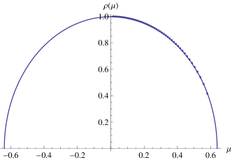
Figure 1: At $t\ll 1$ the eigenvalue density approaches the Wigner distribution ($t=0.1$, $m=50$, $\zeta=0.25$). Solid line: eigenvalue distribution obtained analytically. Dots: numerical solution to (6) with $N=100$.

As $t$ is further increased, the eigenvalue distribution expands and gets flattened forming a plateau, until $t$ gets close to $t\lesssim m$, when two peaks around $\mu\approx\pm m$ begin to form (fig. 2). For finite $R$, small peaks begin to show up already at $t\lesssim m$.

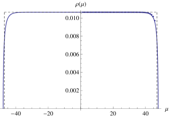
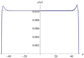
(a)	(b)

Figure 2: Eigenvalue density in phase I for $m=50$, $\zeta=0.25$ and (a) $t=47$, (b) $t=49$. Solid line: analytic solution. Dashed line: solution in the decompactification limit. Dots: numerical solution to (6) with $N=100$.

As the coupling is increased beyond $t=m$, eigenvalues begin to accumulate around $\mu=\pm m$, enhancing the peaks and maintaining the plateau between them (this is shown in fig. 3). This would correspond to phase II in the decompactification limit, where peaks turn into Dirac delta functions. For $\zeta\geq 1$ this phase holds up to $t=\infty$: the eigenvalue distribution is uniform with support in a fixed interval $(-m,m)$, with a density decreasing as $1/t$, and with two peaks at $\mu=\pm m$, whose amplitudes increase until all eigenvalues get on the top of $\mu=\pm m$ as $t\to\infty$.

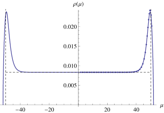
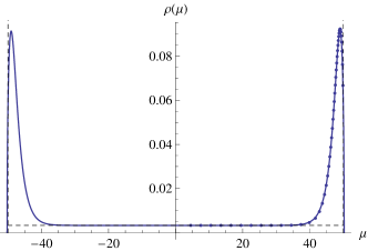
(a)	(b)

Figure 3: Eigenvalue density in phase II for $m=50$ and (a) $t=60$, $\zeta=0.25$, (b) $t=150$, $\zeta=2$ (same conventions as in fig. 2).

When $0<\zeta<1$, phase II holds only in the interval $m<t<m/(1-\zeta)$. For $t>m/(1-\zeta)$, the plateau begins to extend beyond the peaks at $\mu=\pm m$, as shown in fig. 4. Each peak now contains $N_{f}/2$ eigenvalues. This reproduces the behavior found in section 3 for phase III.

Note that fig.3b and 4 display the eigenvalue density for the same value of $t=150$ but different $\zeta$. They illustrate the fact that when $\zeta\geq 1$ eigenvalues lie on the interval $[-m,m]$ for all $t>m$, whereas when $\zeta<1$ the eigenvalue distribution extends beyond $\mu=\pm m$ as soon as $t$ overcomes $m/(1-\zeta)$.

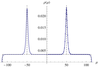
Figure 4: Eigenvalue density in phase III for $m=50$, $t=150$, $\zeta=0.25$ (same conventions as in fig. 2).

Using the eigenvalue density (48), we can obtain the expression for the Wilson loop at finite $R$,

$$W(C) =\frac{1}{t}\sinh^{2}\frac{A}{2}+\frac{\zeta}{2}\frac{\sqrt{1+\cosh m}}{\sqrt{\cosh A+\cosh m}}$$

$$\phantom{=\ }\times\left(\cosh A-1+2\cosh m\left(1-\frac{\sqrt{\cosh A+\cosh m}}{\sqrt{1+\cosh m}}\right)\right)\ .$$ (53)

4.2 Decompactification limit

Let us examine the general formula for the eigenvalue density (48), (49) in the large $R$ limit. It is convenient to restore the $R$ dependence by the scaling $m\to mR$, $A\to AR$, $\mu\to\mu R$. For large $R$, (49) simplifies to the following form

$$A-\frac{1}{R}\log 4=m\lambda(1-\zeta)+\frac{m\lambda\zeta}{\sqrt{e^{(A-m)R}+1}}\ ,$$ (54)

where, again, we have introduced the parameter $\lambda\equiv t/mR$. We now solve this equation in the three different phases:

• $\lambda<1$: Let us assume that $A<m$. In this case we can neglect the exponential inside the square root of (54). This gives $A\approx m\lambda$. Thus the $A<m$ phase appears when $\lambda<1$.

• $1<\lambda<(1-\zeta)^{-1}$: In this interval the solution is of the form:

  $$A=m+\frac{1}{R}\log\left[\frac{\lambda^{2}\zeta^{2}}{(1-\lambda(1-\zeta))^{2}}-1\right]+\mathcal{O}(R^{-2})\ .$$ (55)

  As we will shortly see, the $\mathcal{O}(R^{-1})$ term is important in determining the density at $R\to\infty$. When $\zeta\geq 1$, this solution for $A$ is real for any $\lambda>1$, and in this case this phase extends up to $\lambda=\infty$. When $0<\zeta<1$, (55) solves (54) with real $A$ provided $1<\lambda<(1-\zeta)^{-1}$.

• $\lambda>(1-\zeta)^{-1}$: Let us now assume that $A>m$. In this case the last term of eq. (54) can be neglected and we end up with

  $$A\approx m\lambda(1-\zeta)\ .$$ (56)

  Thus the solution arises only when $\zeta<1$ and $A>m$ requires $\lambda>(1-\zeta)^{-1}$, in concordance with the analysis of section 3.

Consider now the eigenvalue density (48). The first term gives

$$\frac{1}{\pi m\lambda}\tan^{-1}\left(\frac{\sqrt{\cosh AR-\cosh\mu R}}{\sqrt{2}\cosh\frac{\mu R}{2}}\right)\mathop{\longrightarrow}_{R\rightarrow\infty}\left\{\begin{array}[]{lc}0&,\ \ |\mu|=A\ ,\\ \frac{1}{2m\lambda}&,\ \ |\mu|<A\ .\end{array}\right.$$ (57)

Therefore this is the term which gives the plateau, reproducing the same result of section 3.

Consider now the second term in (48). When $A<m$, this term vanishes at large $R$. If, instead, $A>m$, then this term generates two Dirac delta functions centered on $\pm m$ with normalization $\zeta/2$. For a trial function $f(\mu)$, one numerically finds that

$$R\int_{-A}^{A}d\mu\,\frac{2}{\pi}\frac{\cosh\frac{\mu R}{2}\cosh\frac{mR}{2}}{\cosh\mu R+\cosh mR}\frac{\sqrt{\cosh AR-\cosh\mu R}}{\sqrt{\cosh AR+\cosh mR}}\ f(\mu)\ \longrightarrow\ f(m)+f(-m)\ ,$$ (58)

at large $R$.

Finally, consider the intermediate case, phase II, where $A$ is given by (55). We find a similar result as (58), but with an extra overall coefficient $(\lambda-1)/(\zeta\lambda)$. This coefficient is produced by the correction of order $\mathcal{O}(R^{-1})$ in $A$. Thus the resulting $\rho$ exactly matches the solution (16).

In summary, like in ${\cal N}=2$ massive four-dimensional SYM theories, mass deformations in ${\cal N}=2$ supersymmetric three-dimensional Chern-Simons-matter theory lead to new physics involving large $N$ quantum phase transitions. These phase transitions produce non-analytic behavior in supersymmetric observables, like discontinuities in the first derivatives of the vev of the circular Wilson loop, which can be computed explicitly. In this paper we have not included Fayet-Iliopoulos (FI) parameters. Including both FI and mass parameters may shed new light on the properties of the phase transitions. The exchange of mass and FI parameters exchanges mirror pairs of three-dimensional supersymmetric field theories Kapustin:2010xq ; Benvenuti:2011ga . In particular, this indicates that certain massless theories deformed by FI parameters may also exhibit large $N$ phase transitions in some limit. It would be interesting to study the consequences of this interplay in more detail. It would also be interesting to study the analogous decompactification limit in the mass-deformed ABJM partition function given in Kapustin:2010xq .

Acknowledgements

We are grateful to K. Zarembo and M. Mariño for useful comments. The numerical results shown in section 4 were obtained by adapting a Mathematica code developed by Zarembo to the present models. We acknowledge financial support from projects FPA 2010-20807. A.B. also acknowledges support from MECD FPU fellowship AP2009-3511.

References

- (1) V. Pestun, “Localization of gauge theory on a four-sphere and supersymmetric Wilson loops,” Commun. Math. Phys. 313, 71 (2012) [arXiv:0712.2824 [hep-th]].
- (2) A. Kapustin, B. Willett and I. Yaakov, “Exact Results for Wilson Loops in Superconformal Chern-Simons Theories with Matter,” JHEP 1003, 089 (2010) [arXiv:0909.4559 [hep-th]].
- (3) M. Marino, “Lectures on localization and matrix models in supersymmetric Chern-Simons-matter theories,” J. Phys. A 44, 463001 (2011) [arXiv:1104.0783 [hep-th]].
- (4) C. Beasley and E. Witten, “Non-Abelian localization for Chern-Simons theory,” J. Diff. Geom. 70, 183 (2005) [hep-th/0503126].
- (5) N. Drukker, M. Marino and P. Putrov, “From weak to strong coupling in ABJM theory,” Commun. Math. Phys. 306, 511 (2011) [arXiv:1007.3837 [hep-th]].
- (6) J. G. Russo and K. Zarembo, “Localization at Large N,” arXiv:1312.1214 [hep-th].
- (7) J. G. Russo and K. Zarembo, “Evidence for Large-N Phase Transitions in N=2* Theory,” JHEP 1304, 065 (2013) [arXiv:1302.6968 [hep-th]].
- (8) J. G. Russo and K. Zarembo, “Massive N=2 Gauge Theories at Large N,” JHEP 1311, 130 (2013) [arXiv:1309.1004 [hep-th]].
- (9) D. J. Gross and E. Witten, “Possible Third Order Phase Transition in the Large N Lattice Gauge Theory,” Phys. Rev. D 21, 446 (1980).
- (10) S. R. Wadia, “A Study of U(N) Lattice Gauge Theory in 2-dimensions,” arXiv:1212.2906 [hep-th].
- (11) M. Marino, “Les Houches lectures on matrix models and topological strings,” hep-th/0410165.
- (12) C. P. Herzog, I. R. Klebanov, S. S. Pufu and T. Tesileanu, Phys. Rev. D 83, 046001 (2011) [arXiv:1011.5487 [hep-th]].
- (13) R. C. Santamaria, M. Marino and P. Putrov, “Unquenched flavor and tropical geometry in strongly coupled Chern-Simons-matter theories,” JHEP 1110, 139 (2011) [arXiv:1011.6281 [hep-th]].
- (14) D. L. Jafferis, I. R. Klebanov, S. S. Pufu and B. R. Safdi, “Towards the F-Theorem: N=2 Field Theories on the Three-Sphere,” JHEP 1106, 102 (2011) [arXiv:1103.1181 [hep-th]].
- (15) J. H. Schwarz, “Superconformal Chern-Simons theories,” JHEP 0411, 078 (2004) [hep-th/0411077].
- (16) D. Gaiotto and X. Yin, “Notes on superconformal Chern-Simons-Matter theories,” JHEP 0708, 056 (2007) [arXiv:0704.3740 [hep-th]].
- (17) A. Kapustin, B. Willett and I. Yaakov, “Nonperturbative Tests of Three-Dimensional Dualities,” JHEP 1010, 013 (2010) [arXiv:1003.5694 [hep-th]].
- (18) J. G. Russo and K. Zarembo, “Large N Limit of N=2 SU(N) Gauge Theories from Localization,” JHEP 1210, 082 (2012) [arXiv:1207.3806 [hep-th]].
- (19) A. Buchel, J. G. Russo and K. Zarembo, “Rigorous Test of Non-conformal Holography: Wilson Loops in N=2* Theory,” JHEP 1303, 062 (2013) [arXiv:1301.1597 [hep-th]].
- (20) S. Benvenuti and S. Pasquetti, “3D-partition functions on the sphere: exact evaluation and mirror symmetry,” JHEP 1205, 099 (2012) [arXiv:1105.2551 [hep-th]].