The existence of designs

Abstract

We prove the existence conjecture for combinatorial designs, answering a question of Steiner from 1853. More generally, we show that the natural divisibility conditions are sufficient for clique decompositions of uniform hypergraphs that satisfy a certain pseudorandomness condition. As a further generalisation, we obtain the same conclusion only assuming an extendability property and the existence of a robust fractional clique decomposition.

1 Introduction

A Steiner system with parameters $(n,q,r)$ is a set $S$ of $q$-subsets of an $n$-set $X$, such that every $r$-subset of $X$ belongs to exactly one element of $S$. The question of whether there is a Steiner system with given parameters is one of the oldest problems in combinatorics, dating back to work of Plücker (1835), Kirkman (1846) and Steiner (1853); see [39] for a historical account.

More generally, we say that a set $S$ of $q$-subsets of an $n$-set $X$ is a design with parameters $(n,q,r,\lambda)$ if every $r$-subset of $X$ belongs to exactly $\lambda$ elements of $S$. (This is often called an ‘$r$-design’ in the literature.) There are some obvious necessary ‘divisibility conditions’ for the existence of such $S$, namely that $\tbinom{q-i}{r-i}$ divides $\lambda\tbinom{n-i}{r-i}$ for every $0\leq i\leq r-1$ (fix any $i$-subset $I$ of $X$ and consider the sets in $S$ that contain $I$). It is not known who first advanced the ‘Existence Conjecture’ that the divisibility conditions are also sufficient, apart from a finite number of exceptional $n$ given fixed $q$, $r$ and $\lambda$.

The case $r=2$ has received particular attention due to its connections to statistics, under the name of ‘balanced incomplete block designs’. We refer the reader to [4] for a summary of the large literature and applications of this field. The Existence Conjecture for $r=2$ was a long-standing open problem, eventually resolved by Wilson [42, 43, 44] in a series of papers that revolutionised Design Theory, and had a major impact in Combinatorics. In this paper, we prove the Existence Conjecture in general, via a new method, which we will refer to as Randomised Algebraic Constructions.

1.1 Results

The Existence Conjecture will follow from a more general result on clique decompositions of hypergraphs that satisfy a certain pseudorandomness condition. To describe this we make the following definitions.

Definition 1.1.

A hypergraph $G$ consists of a vertex set $V(G)$ and an edge set $E(G)$, where each $e\in E(G)$ is a subset of $V(G)$. We identify $G$ with $E(G)$. If every edge has size $r$ we say that $G$ is an $r$-graph. For $S\subseteq V(G)$, the neighbourhood $G(S)$ is the $(r-|S|)$-graph $\{f\subseteq V(G)\setminus S:f\cup S\in G\}$. For an $r$-graph $H$, an $H$-decomposition of $G$ is a partition of $E(G)$ into subgraphs isomorphic to $H$. Let $K^{r}_{q}$ be the complete $r$-graph on $q$ vertices.

Note that a Steiner system with parameters $(n,q,r)$ is equivalent to a $K^{r}_{q}$-decomposition of $K^{r}_{n}$. It is also equivalent to a perfect matching (a set of edges covering every vertex exactly once) in the auxiliary $\tbinom{q}{r}$-graph on $\tbinom{[n]}{r}$ (the $r$-subsets of $[n]:=\{1,\dots,n\}$) with edge set $\{\tbinom{Q}{r}:Q\in\tbinom{[n]}{q}\}$. The next definition generalises the necessary divisibility conditions described above.

Definition 1.2.

Suppose $G$ is an $r$-graph. We say that $G$ is $K^{r}_{q}$-divisible if $\tbinom{q-i}{r-i}$ divides $|G(e)|$ for any $i$-set $e\subseteq V(G)$, for all $0\leq i\leq r$.

Next we formulate our quasirandomness condition. It is easy to see that it holds whp if $G=G^{r}(n,p)$ is the standard binomial random $r$-graph and $n$ is large given $p$, $c$ and $h$.

Definition 1.3.

Suppose $G$ is an $r$-graph on $[n]$. The density of $G$ is $d(G)=|G|\tbinom{n}{r}^{-1}$. We say that $G$ is $(c,h)$-typical if for any set $A$ of $(r-1)$-subsets of $V(G)$ with $|A|\leq h$ we have $\left|\cap_{S\in A}G(S)\right|=(1\pm|A|c)d(G)^{|A|}n$.

Now we can state a simplified form of our main theorem.

Theorem 1.4.

For any $q>r\geq 1$ there are $c_{0},\alpha>0$ and $h,n_{0}\in\mathbb{N}$ so that if $G$ is a $K^{r}_{q}$-divisible $(c,h)$-typical $r$-graph on $n>n_{0}$ vertices, where $d(G)>n^{-\alpha}$ and $c<c_{0}d(G)^{h^{2}}$, then $G$ has a $K^{r}_{q}$-decomposition.

Applying this with $G=K^{r}_{n}$, we deduce that for large $n$ the divisibility conditions are sufficient for the existence of Steiner systems; the existence of designs with any constant multiplicity $\lambda$ follows from Theorem 1.10 below. We have not tried to optimise our parameters, although we do emphasise that the density of $G$ can decay polynomially in $n$, as this is used in [22] to estimate the number of designs. Our method gives a randomised algorithm for constructing designs.

Theorem 1.4 gives new results even in the graph case ($r=2$); for example, it is easy to deduce that the standard random graph model $G(n,1/2)$ whp has a partial triangle decomposition that covers all but $(1+o(1))n/4$ edges: deleting a perfect matching on the set of vertices of odd degree and then at most two $4$-cycles (to make the number of edges divisible by $3$) gives a graph satisfying the hypotheses of the theorem. This is the asymptotically best possible ‘leave’, as whp there are $(1+o(1))n/2$ vertices of odd degree and any partial triangle decomposition must leave at least one edge uncovered at each vertex of odd degree.

We also note that if an $r$-graph $G$ on $n$ vertices satisfies $|G(S)|\geq(1-c)n$ for every $(r-1)$-subset $S$ of $V(G)$ then it is $(c,h)$-typical, so we also deduce a minimum $(r-1)$-degree version of the theorem, generalising Gustavsson’s minimum degree version [14] of Wilson’s theorem.

To state our main theorem we introduce the following more general context of $r$-multigraphs. Note that an $(n,q,r,\lambda)$-design is equivalent to a $K^{r}_{q}$-decomposition of the $r$-multigraph $\lambda\tbinom{[n]}{r}$.

Definition 1.5.

An $r$-multigraph $G$ on $[n]$ is a multiset in which each element is an $r$-subset of $[n]$. We identify $G$ with a vector $G\in\mathbb{N}^{K^{r}_{n}}$, where $G_{e}$ is the multiplicity of $e$ in $G$.

We can also relax our pseudorandomness assumption, with essentially the same proof, obtaining a more general result in the spirit of [25], i.e. that under certain conditions (‘extendability’ and ‘robust fractional decomposition’), divisibility is the only obstruction to decomposition. The next two definitions formulate our extendability assumption (see subsection 2.3 for more discussion).

Definition 1.6.

Suppose $H$ is an $r$-graph, $G$ is an $r$-multigraph on $[n]$ and $\phi:V(H)\to[n]$ is injective. We call $\phi$ an embedding of $H$ in $G$ if $G_{\phi(f)}>0$ for all $f\in H$. We write $K^{r}_{q}(G)$ for the set of $\phi(Q)$ where $\phi$ is an embedding of $Q=K^{r}_{q}$ in $G$.

Definition 1.7.

Suppose $H$ is an $r$-graph, $F\subseteq V(H)$ and $\phi:F\to[n]$ is injective. We call $E=(\phi,F,H)$ an extension. We write $e_{E}=|H\setminus H[F]|$, $v_{E}=|V(H)\setminus F|$ and call $e_{E}$ the rank of $E$. Now suppose $G$ is an $r$-multigraph on $[n]$. We write $X_{E}(G)$ for the set or number of embeddings of $H$ in $G+\phi(H[F])$ that restrict to $\phi$ on $F$. We say $E$ is $\omega$-dense (in $G$) if $X_{E}(G)\geq\omega n^{v_{E}}$. We say $G$ is $(\omega,h)$-extendable if all extensions of rank $h$ are $\omega$-dense in $G$.

Next we formulate our robust fractional decomposition assumption.

Definition 1.8.

An $r$-multigraph $G$ on $[n]$ is $(K^{r}_{q},c,\omega)$-regular if there are $w_{Q^{\prime}}\in[\omega n^{r-q},\omega^{-1}n^{r-q}]$ for each $Q^{\prime}\in K^{r}_{q}(G)$ with $\sum\{w_{Q^{\prime}}:e\in Q^{\prime}\}=(1\pm c)G_{e}$ for all $e\in\tbinom{[n]}{r}$.

Note in particular that the upper bounds $w_{Q^{\prime}}\leq\omega^{-1}n^{r-q}$ in Definition 1.8 imply $G_{e}\leq\omega^{-1}$ for all $e\in K^{r}_{n}$. We also reformulate our divisibility assumption so that it applies to $r$-multigraphs $J\in\mathbb{N}^{K^{r}_{n}}$, and more generally any $J\in\mathbb{Z}^{K^{r}_{n}}$.

Definition 1.9.

Suppose $J\in\mathbb{Z}^{K^{r}_{n}}$. We say that $J$ is $K^{r}_{q}$-divisible if $\tbinom{q-i}{r-i}$ divides $\sum\{J_{e}:f\subseteq e\}$ for any $0\leq i\leq r$, $f\in\tbinom{[n]}{i}$.

Finally, we state our main theorem.

Theorem 1.10.

For any $q>r\geq 1$ there are $c_{0}>0$ and $n_{0}\in\mathbb{N}$ so that if $h=2^{50q^{3}}$, $b=2^{3^{r+q}}$, $n>n_{0}$, $n^{-b^{-1}h^{-2}}<\omega<1$ and $c<c_{0}\omega^{h}$ then any $K^{r}_{q}$-divisible $(K^{r}_{q},c,\omega)$-regular $(\omega,h)$-extendable $r$-multigraph on $n$ vertices has a $K^{r}_{q}$-decomposition.

1.2 Related work

As a weaker version of the Existence Conjecture, Erdős and Hanani [5] asked for approximate Steiner systems; equivalently, finding $(1-o(1))\tbinom{q}{r}^{-1}\tbinom{n}{r}$ edge-disjoint $K^{r}_{q}$’s in $K^{r}_{n}$. This was solved by Rödl [35], who introduced a semi-random construction method known as the ‘nibble’, which has since had a great impact on Combinatorics (see e.g. [1, 7, 12, 18, 26, 27, 30, 34, 40, 41] for related results and improved bounds). It will also play an important role in this paper.

Regarding exact results, we have already mentioned Wilson’s theorem, and Gustavsson’s minimum degree generalisation thereof. We should also note the seminal work of Hanani [15, 16], which (inter alia) answers Steiner’s problem for $(q,r)\in\{(4,2),(4,3),(5,2)\}$ and all $n$ (the case $(q,r)=(3,2)$ was solved by Kirkman, before Steiner posed the problem). Besides these, we again refer to [4] as an introduction to the huge literature on the construction of designs. One should note that before the results of the current paper, there were only finitely many known Steiner systems with $r\geq 4$, and it was not known if there were any Steiner systems with $r\geq 6$.

Even the existence of designs with $r\geq 7$ and any ‘non-trivial’ $\lambda$ was open before the breakthrough result of Teirlinck [38] confirming this. An improved bound on $\lambda$ and a probabilistic method (a local limit theorem for certain random walks in high dimensions) for constructing many other rigid combinatorial structures was recently given by Kuperberg, Lovett and Peled [29]. Their result for designs is somewhat complementary to ours, in that they can allow the parameters $q$ and $r$ to grow with $n$, whereas we require them to be (essentially) constant. They also obtain much more precise estimates than we do for the number of designs (within their range of parameters). Another recent result, due to Ferber, Hod, Krivelevich and Sudakov [6] gives a short probabilistic construction of ‘almost Steiner systems’, in which every $r$-subset is covered by either one or two $q$-subsets.

A different relaxation of the conjecture, which will play an important role in this paper, is obtained by considering ‘integral designs’, in which one assigns integers to the copies of $K^{r}_{q}$ in $K^{r}_{n}$ such that for every edge $e$ the sum of the integers assigned to the copies of $K^{r}_{q}$ containing $e$ is a constant independent of $e$. Graver and Jurkat [13] and Wilson [45] showed that the divisibility conditions suffice for the existence of integral designs (this is used in [45] to show the existence for large $\lambda$ of integral designs with non-negative coefficients). Wilson [46] also characterised the existence of integral $H$-decompositions for any $r$-graph $H$.

Over the years since the first version [21] of this paper was made available there have been many further related developments. We omit discussion of most of these (a separate survey article would be needed to do justice to this task), except to mention two subsequent papers in which the new method of this paper (discussed below) plays a key role: a conjectural analogue of the ‘expander mixing lemma’ for ‘high-dimensional permutations’ proposed by Linial and Luria [32], and a result of Kwan [31] on the existence of perfect matchings in random Steiner Triple Systems. We also remark that Glock, Kühn, Lo and Osthus [9, 10] have recently given a new proof of our main result, as well as some generalisations, such as the existence of $H$-decompositions for any hypergraph $H$ (a question from [21]); we will compare our approach with theirs below.

1.3 Proof strategy

Our main new idea is to use a Randomised Algebraic Construction: the first step of our construction is to take a random subset of an algebraically defined ‘model’ for designs. This results in a partial decomposition that covers a constant fraction of the edge set, and also carries a rich structure of possible local modifications. We treat this partial decomposition as a template for the final decomposition. By various applications of the nibble and greedy algorithms, we can choose another partial decomposition that covers all edges not in the template, which also spills over slightly into the template, so that every edge is covered once or twice, and very few edges are covered twice (we call the latter the ‘spill’). The crucial point is that the choice of the template was such that the spill can be ‘absorbed’, converting the approximate decomposition into a (perfect) decomposition.

At this level of generality, our method sounds somewhat similar to the Absorbing Method of Rödl, Ruciński and Szemerédi [37] (see also the survey [36]). However, in the Absorbing Method (in its basic form) as applied to the problem of designs, the analogue of our template would be a random sparse partial decomposition (without any superimposed algebraic structure), and it is not hard to see that local modifications have a negligible probability of appearing in such a construction. Another way to think about the failure of the Absorbing Method is that there are too many possibilities for the ‘leave’ of the approximate decomposition. This viewpoint suggests the more sophisticated approach of Iterative Absorption used in [9], in which the leave becomes gradually more constrained, until there are so few options that each possible leave can have its own private ‘absorber’. (Iterative Absorption has recently been a powerful tool for many other problems; see the survey [28].)

By contrast, our construction blends randomness with algebra, in a way that any approximation to a decomposition can be absorbed. The rich rigid structures of Algebra make it a natural tool in the construction of designs. For example, orbits of $r$-transitive permutation groups give immediate constructions of $r$-designs, but (according to the Classification of Finite Simple Groups) there are no $r$-transitive groups with $r>5$ other than the symmetric and alternating groups, which points to the limitations of the purely algebraic approach.

Nevertheless, we will see that a suitable algebraically defined template has a dense well-distributed set of cliques that are ‘absorbable’, in that they can be included in the clique decomposition of the template via a suitable local modification. To make use of this structure, we first find an ‘integral decomposition’ of the spill, which can be thought of as a decomposition in which we can take each clique with any integer weight; this is the point in the proof where the divisibility assumption is used. Next we apply a ‘clique exchange algorithm’ that replaces the integral decomposition by a ‘signed decomposition’, which can be thought of as two partial decompositions, called ‘positive’ and ‘negative’, such that the underlying hypergraph of the negative decomposition is contained in that of the positive decomposition, and the difference forms a ‘hole’ that is precisely equal to the spill. We further ensure that each positive clique can be absorbed into the template, via a series of absorptions that we call a ‘cascade’. Finally, deleting the positive cliques and replacing them by the negative cliques eliminates one of the two uses of each edge in the spill, so that we end up with a perfect decomposition.

1.4 Implementation

While the overall proof strategy in this version of the paper is the same as in the first version [21], the details of the implementation here are substantially different and considerably simpler. The most important difference is that we now do not need any inductive argument for reducing the vertex set. There was an error in this part of our argument in [21], which was kindly pointed out by the authors of [9], namely in the proof of [21, Lemma 6.3]. The lemma is true, and the proof can be fixed with more sophisticated random greedy arguments, but this would make [21] even more complicated, whereas the issue is entirely avoided by our new approach. Furthermore, we can work entirely in the simpler setting of uniform hypergraphs, rather than the more general setting of simplicial complexes that was needed in [21] for the purposes of induction. The simpler method presented here may also be more amenable to computer implementation with a view to constructing explicit designs.

To develop some intuition for Randomised Algebraic Construction it is helpful to first consider the special case of triangle decompositions of typical graphs (see [22]). Our algebraic model for triangle decompositions is the set of all triples $xyz$ with $x+y+z=0$ in some abelian group $\Gamma$. Indeed, this is almost a triangle decomposition of the complete graph on $\Gamma$, in that for any $xy$ there is a unique $z$ with $x+y+z=0$, but this ignores the possibility that $x,y,z$ may not be distinct, and also that our approach requires decompositions of (hyper)graphs that are not complete. Instead, to define the template of a graph $G$ in [22], we randomly embed $V(G)$ in $\mathbb{F}_{2^{a}}$ for some $a$ such that $2^{a}$ is not much bigger than $|V(G)|$, and take all triangles $xyz$ satisfying $x+y+z=0$, which gives a partial triangle decomposition of $G$. In this construction, a triangle $uvw$ is absorbable if $G$ contains the ‘associated octahedron’ of $uvw$, which is the complete $3$-partite graph with parts $\{u,v+w\}$, $\{v,w+u\}$, $\{w,u+v\}$. Indeed, this octahedron has two distinct triangle decompositions, one of which contains $uvw$, and the other of which consists entirely of triangles with zero sum.

In general, for our algebraic model of a $K^{r}_{q}$-decomposition, we consider a vertex set that is a finite field, and a set of $q$-cliques that correspond to the image of some $q\times r$ matrix $M$ that is ‘generic’ (every square submatrix of $M$ is nonsingular). The motivation for this model is that for every $r$-set $e$ of field elements and injective map $\pi_{e}:e\to[q]$, we can reconstruct the unique vector $y$ such that $(My)_{i}=x$ for all $x\in e$, $i=\pi_{e}(x)$. However, if we embed some $r$-graph $G$ in the field and use this construction, then as in the triangle decomposition case, we can only use the subset of the model that uses edges which are actually present in the given $r$-graph $G$. Furthermore, as we must use each edge at most once, we make each edge $e$ randomly ‘decide’ on some fixed injection $\pi_{e}$, and we only allow $q$-cliques that are compatible with these choices.

Similarly to the case of triangle decompositions, we randomly embed $V(G)$ in $\mathbb{F}_{p^{a}}$, for some prime $p$ which is large compared with $q$ but small compared with $n=|V(G)|$, and some $a$ such that $p^{a}$ is not much bigger than $n$. Viewing $\mathbb{F}_{p^{a}}$ as a vector space over $\mathbb{F}_{p}$ we find a rich set of absorbable cliques via a construction somewhat analogous to the associated octahedra of triangles (this part of the argument is new to this version and is much simpler than the approach used in the first version). In fact, rather than using just using one embedding of $V(G)$ in $\mathbb{F}_{p^{a}}$, we use $z$ such embeddings, for some $z$ which is large compared with $q$ but small compared with $n$. The point of this is that with positive probability every $r$-set has full $\mathbb{F}_{p}$-dimension in most of these embeddings, which circumvents many technical difficulties from the first version regarding the treatment of degenerate sets.

Our final comment on the new implementation is that we have found a considerably simpler approach for constructing ‘bounded integral designs’. As described above, Graver and Jurkat [13] and Wilson [45] showed that the divisibility conditions suffice for the existence of integral designs, but our modification approach requires an additional local boundedness property. Our new approach for bounded integral designs relies on ‘robust local decodability’ of the lattice of $K^{r}_{q}$-divisible vectors: there is some constant $N=N(q)$ such that for any $e\in K^{r}_{n}$ there are ‘many’ integral combinations of $q$-cliques that equal the vector in $\mathbb{Z}^{K^{r}_{n}}$ with $N$ in coordinate $e$ and $0$ otherwise.

It is interesting that local decodability was a key property in the general framework of [29], although we do not see any connection between this part of our proof and their approach. Furthermore, there are many natural related problems in design theory that do not exhibit local decodability, such as ‘generalised partite hypergraph decompositions’, which encompass problems such as resolvable hypergraph designs, large sets of hypergraph designs, decompositions of designs by designs, high-dimensional permutations and Sudoku squares (see [23]). Here the method from the first version of this paper can be applied: the key idea is to solve the fractional relaxation of the integral design problem (we allow rational weights of either sign), and use this in an iterative rounding algorithm to obtain finer approximations to an exact solution until the approximation is so good that a trivial argument can be used to complete the solution. However, the general integral relaxation has a much more complicated structure, so there are many further difficulties to overcome (see [23]).

1.5 Organisation

The organisation of this paper is as follows. The next section contains various preliminary results used throughout the paper, on concentration of probability, almost perfect matchings in hypergraphs, and extensions. In section 3 we construct the template, and establish its combinatorial extendability properties. Section 4 contains the nibble and cover arguments that complete the template to an approximate decomposition, namely a set of cliques such that every edge is covered once or twice, and the set of edges covered twice (the ‘spill’) forms a suitably bounded subgraph of the template. In section 5 we find a suitably bounded integral decomposition of the spill. In section 6 we analyse the algebraic properties of the template, showing that it has a rich structure of absorbable and cascading cliques that can be used for local modifications. Section 7 analyses the Clique Exchange Algorithm that modifies the integral decomposition so that the spill can be absorbed into the template. In the final section we complete the proof of our main theorem and make some concluding remarks.

1.6 Notation and terminology

Here we gather some notation and terminology that is used throughout the paper. We write $[n]=\{1,\dots,n\}$. For a set $S$, we write $\tbinom{S}{r}$ for the set of $r$-subsets of $S$. We write $Q=\tbinom{[q]}{r}$ and also $Q=\tbinom{q}{r}$ (it will be clear from the context whether we are referring to the set or its size). We identify $Q=\tbinom{[q]}{r}$ with the edge set of $K^{r}_{q}$ (the complete $r$-graph on $[q]$).

For any set $S$ we write $K^{r}_{q}(S)$ for the complete $q$-partite $r$-graph with parts of size $|S|$ where each part is identified with $S$. If $S=[s]$ we write $K^{r}_{q}(S)=K^{r}_{q}(s)$.

We often use ‘concatenation notation’ for sets, for example $xyz$ may denote $\{x,y,z\}$, and for function composition, for example $fg$ may denote $f\circ g$.

We say that an event $E$ holds with high probability (whp) if $\mathbb{P}(E)=1-e^{-\Omega(n^{c})}$ for some $c>0$ as $n\to\infty$. Whenever we make any such statement, we are implicitly assuming that $n>n_{0}(q)$ is sufficiently large. Then by union bounds we can assume that any specified polynomial number of such events all occur.

Suppose $X$ and $Y$ are sets. We write $Y^{X}$ for the set of vectors with entries in $Y$ and coordinates indexed by $X$, which we also identify with the set of functions $f:X\to Y$. For example, we may consider $v\in\mathbb{F}_{p}^{q}$ as an element of a vector space over $\mathbb{F}_{p}$ or as a function from $[q]$ to $\mathbb{F}_{p}$.

We identify $v\in\{0,1\}^{X}$ with the set $\{x\in X:v_{x}=1\}$. We identify $v\in\mathbb{N}^{X}$ with the multiset in $X$ in which $x$ has multiplicity $v_{x}$ (for our purposes $0\in\mathbb{N}$). We also apply similar notation and terminology as for multisets to vectors $v\in\mathbb{Z}^{X}$ (which one might call ‘intsets’). We often consider algorithms with input $v\in\mathbb{Z}^{X}$, where each $x\in X$ is considered $|v_{x}|$ times, with a sign attached to it (the same as that of $v_{x}$); then we refer to $x$ as a ‘signed element’ of $v$.

Arithmetic on vectors in $\mathbb{Z}^{X}$ is to be understood pointwise, i.e. $(v+v^{\prime})_{x}=v_{x}+v^{\prime}_{x}$ and $(vv^{\prime})_{x}=v_{x}v^{\prime}_{x}$ for $x\in X$. For $v\in\mathbb{Z}^{X}$ we write $|v|=\sum_{x\in X}|v_{x}|$. We also write $v=v^{+}-v^{-}$, where $v^{+}_{x}=\max\{v_{x},0\}$ and $v^{-}_{x}=\max\{-v_{x},0\}$ for $x\in X$. For $X^{\prime}\subseteq X$ we define $v[X^{\prime}]\in\mathbb{Z}^{X^{\prime}}$ by $v[X^{\prime}]_{x}=v_{x}$ for $x\in X^{\prime}$.

If $G$ is a hypergraph, $v\in\mathbb{Z}^{G}$ and $e\in G$ we define $v(e)\in\mathbb{Z}^{G(e)}$ by $v(e)_{f}=v_{e\cup f}$ for $f\in G(e)$.

We say $J\in\mathbb{Z}^{K^{r}_{n}}$ is $\theta$-bounded if $\sum\{|J_{e}|:f\subseteq e\in K^{r}_{n}\}<\theta n$ for all $f\in\tbinom{[n]}{r-1}$.

We denote the standard basis vectors in $\mathbb{R}^{d}$ by $e_{1},\dots,e_{d}$. Given $I\subseteq[d]$, we let $e_{I}$ denote the $I$ by $[d]$ matrix in which the row indexed by $i\in I$ is $e_{i}$.

We write $M\in\mathbb{F}_{p}^{q\times r}$ to mean that $M$ is a matrix with $q$ rows and $r$ columns having entries in $\mathbb{F}_{p}$. For $I\in Q=\tbinom{[q]}{r}$ we let $M_{I}$ be the square submatrix with rows indexed by $I$. Note that $M_{I}=e_{I}M$.

We will regard $\mathbb{F}_{p^{a}}$ as a vector space over $\mathbb{F}_{p}$. For $e\subseteq\mathbb{F}_{p^{a}}$ we write $\dim(e)$ for the dimension of the subspace spanned by the elements of $e$. For $e\in\mathbb{F}_{p^{a}}^{d}$ we write $\dim(e)$ for the dimension of the set of coordinates of $e$.

When we use ‘big-O’ notation, the implicit constant will depend only on $q$.

We write $a=b\pm c$ to mean $b-c\leq a\leq b+c$.

Throughout the paper we omit floor and ceiling symbols where they do not affect the argument.

For convenient reference, we list here several parameters used throughout the paper:

$$Q=\tbinom{q}{r},\quad z=h=2^{50q^{3}},\quad b=2^{3^{r+q}},\quad n^{-b^{-1}h^{-2}}<\omega<\omega_{0}(q),\quad p\text{ is a prime with }2^{8q}<p<2^{9q},$$

$$a\in\mathbb{N}\text{ with }p^{a-2}<n\leq p^{a-1},\quad\gamma=np^{-a},\quad\rho=\omega z^{-Q}q!(q)_{r}^{-Q}\gamma^{q-r},\text{ where }(q)_{r}=q!/(q-r)!,$$

$$N=(2q)^{q}!,\quad c=\omega^{h},\quad c_{1}=(2Qc)^{1/2Q},\quad c_{i+1}=\omega^{-h/20Q}c_{i}\ \text{ for }\ i\in[4].$$

The multiplicative factor of $\omega^{-h/20Q}$ between successive $c_{i}$’s is chosen so that there is plenty of room to spare in the various inequalities below, so we will omit detailed discussion of these during the proof. We remark here that the tightest inequality occurs during the cascade algorithm in the proof of Theorem 1.10, namely $2^{r}p^{2q}r!\omega^{-p^{q^{2}}}c_{4}<c_{5}/12$, which holds easily as $p^{q^{2}}<2^{9q^{3}}<h^{1/5}$ and $Q<q^{q}<2^{q^{2}}=h^{1/50q}$. The assumption $\omega>n^{-b^{-1}h^{-2}}$ is much stronger than needed for the proof, but we are only interested in establishing some polynomial dependence, as in any case the best bounds available from our proof are presumably far from optimal.

2 Preliminaries

In this section we gather some results that will be used throughout the paper, concerning concentration of probability, almost perfect matchings in hypergraphs, and extensions.

2.1 Concentration of probability

We make the following standard definitions.

Definition 2.1.

Let $\Omega$ be a (finite) probability space. An algebra (on $\Omega$) is a set $\mathcal{F}$ of subsets of $\Omega$ that includes $\Omega$ and is closed under intersections and taking complements. A filtration (on $\Omega$) is a sequence $\mathcal{F}=(\mathcal{F}_{i})_{i\geq 0}$ of algebras such that $\mathcal{F}_{i}\subseteq\mathcal{F}_{i+1}$ for $i\geq 0$. A sequence $A=(A_{i})_{i\geq 0}$ of random variables on $\Omega$ is a supermartingale (wrt $\mathcal{F}$) if each $A_{i}$ is $\mathcal{F}_{i}$-measurable (all $\{\omega:A_{i}(\omega)<t\}\in\mathcal{F}_{i}$) and $\mathbb{E}(A_{i+1}|\mathcal{F}_{i})\leq A_{i}$ for $i\geq 0$.

Now we can state a general result of Freedman [8, Proposition 2.1] that essentially implies all of the bounds we will use (perhaps with slightly weaker constants).

Lemma 2.2.

Let $(A_{i})_{i\geq 0}$ be a supermartingale wrt a filtration $\mathcal{F}=(\mathcal{F}_{i})_{i\geq 0}$. Suppose that $A_{i+1}-A_{i}\leq b$ for all $i\geq 0$, and let $E$ be the ‘bad’ event that there exists $j\geq 0$ with $A_{j}\geq A_{0}+a$ and $\sum_{i=1}^{j}Var[A_{i}\mid\mathcal{F}_{i-1}]\leq v$. Then $\mathbb{P}(E)\leq\exp\left(-\tfrac{a^{2}}{2(v+ab)}\right)$.

We proceed to give some useful consequences of Lemma 2.2. First we make another definition.

Definition 2.3.

Suppose $Y$ is a random variable and $\mathcal{F}=(\mathcal{F}_{0},\dots,\mathcal{F}_{n})$ is a filtration. We say that $Y$ is $(C,\mu)$-dominated (wrt $\mathcal{F}$) if we can write $Y=\sum_{i=1}^{n}Y_{i}$, where $Y_{i}$ is $\mathcal{F}_{i}$-measurable, $|Y_{i}|\leq C$ and $\mathbb{E}[|Y_{i}|\mid\mathcal{F}_{i-1}]<\mu_{i}$ for $i\in[n]$, where $\sum_{i=1}^{n}\mu_{i}<\mu$.

Lemma 2.4.

If $Y$ is $(C,\mu)$-dominated then $\mathbb{P}(|Y|>(1+c)\mu)<2e^{-\mu c^{2}/2(1+2c)C}$.

Proof. Let $A_{i}=\sum_{j<i}(Y_{j}-\mu_{j})$ for $i\geq 0$; then $(A_{i})_{i\geq 0}$ is a supermartingale and

$$Var[A_{i}\mid\mathcal{F}_{i-1}]=Var[Y_{i}\mid\mathcal{F}_{i-1}]\leq\mathbb{E}[Y_{i}^{2}\mid\mathcal{F}_{i-1}]\leq C\mathbb{E}[|Y_{i}|\mid\mathcal{F}_{i-1}]\leq C\mu_{i}.$$

By Lemma 2.2 applied with $a=c\mu$, $b=2C$ and $v=C\mu$ we obtain

$$\mathbb{P}(Y>(1+c)\mu)<e^{-\mu c^{2}/2(1+2c)C}.$$

Similarly, considering $A_{i}=-\sum_{j<i}(Y_{j}+\mu_{j})$ gives the same estimate for $\mathbb{P}(Y<-(1+c)\mu)$. $\Box$

Remark 2.5.

All of our applications of Lemma 2.4 will be such that we could also deduce concentration by coupling to a sum of bounded independent variables. In many cases, we will actually have a sum of bounded independent variables (i.e. there is no need for a coupling), in which case we will simply refer to the standard ‘Chernoff bound’ (see e.g. [17, Remark 2.9]). For brevity we call such variables ‘pseudobinomial’.

Next we record several consequences of the well-known inequality of Azuma [2] (see e.g. [33]).

Definition 2.6.

Suppose $f:S\to\mathbb{R}$ where $S=\prod_{i=1}^{n}S_{i}$ and $b=(b_{1},\dots,b_{n})$ with $b_{i}\geq 0$ for $i\in[n]$. We say that $f$ is $b$-Lipschitz if for any $s,s^{\prime}\in S$ that differ only in the $i$th coordinate we have $|f(s)-f(s^{\prime})|\leq b_{i}$. We also say that $f$ is $B$-varying where $B=\sum_{i=1}^{n}b_{i}^{2}$.

Lemma 2.7.

Suppose $Z=(Z_{1},\dots,Z_{n})$ is a sequence of independent random variables, and $X=f(Z)$, where $f$ is a $B$-varying function. Then $\mathbb{P}(|X-\mathbb{E}X|>a)\leq 2e^{-a^{2}/2B}$.

Definition 2.8.

Let $S_{n}$ be the symmetric group on $[n]$. Suppose $f:S_{n}\to\mathbb{R}$ and $b\geq 0$. We say that $f$ is $b$-Lipschitz if whenever $\sigma=\tau\circ\sigma^{\prime}$ for some transposition $\tau\in S_{n}$ we have $|f(\sigma)-f(\sigma^{\prime})|\leq b$.

Lemma 2.9.

Suppose $f:S_{n}\to\mathbb{R}$ is $b$-Lipschitz, $\sigma\in S_{n}$ is uniformly random and $X=f(\sigma)$. Then $\mathbb{P}(|X-\mathbb{E}X|>a)\leq 2e^{-a^{2}/2nb^{2}}$.

We will use a common generalisation of Lemmas 2.7 and 2.9, which perhaps has not appeared before, but is proved in the same way. It considers functions in which the input consists of $n$ independent random injections $\pi_{i}:[a^{\prime}_{i}]\to[a_{i}]$: if $a^{\prime}_{i}=1$ this is a random element of $[a_{i}]$; if $a^{\prime}_{i}=a_{i}$ this is a random permutation of $[a_{i}]$.

Definition 2.10.

Let $a=(a_{1},\dots,a_{n})$ and $a^{\prime}=(a^{\prime}_{1},\dots,a^{\prime}_{n})$, where $a_{i}\in\mathbb{N}$ and $a^{\prime}_{i}\in[a_{i}]$ for $i\in[n]$, and $\Pi(a,a^{\prime})$ be the set of $\pi=(\pi_{1},\dots,\pi_{n})$ where $\pi_{i}:[a^{\prime}_{i}]\to[a_{i}]$ is injective. Suppose $f:\Pi(a,a^{\prime})\to\mathbb{R}$ and $b=(b_{1},\dots,b_{n})$ with $b_{i}\geq 0$ for $i\in[n]$. We say that $f$ is $b$-Lipschitz if for any $i\in[n]$ and $\pi,\pi^{\prime}\in\Pi(a,a^{\prime})$ such that $\pi_{j}=\pi^{\prime}_{j}$ for $j\neq i$ and $\pi_{i}=\tau\circ\pi^{\prime}_{i}$ for some transposition $\tau\in S_{a_{i}}$ we have $|f(s)-f(s^{\prime})|\leq b_{i}$. We also say that $f$ is $B$-varying where $B=\sum_{i=1}^{n}a^{\prime}_{i}b_{i}^{2}$.

Lemma 2.11.

Suppose $f:\Pi(a,a^{\prime})\to\mathbb{R}$ is $B$-varying, $\pi\in\Pi(a,a^{\prime})$ is uniformly random and $X=f(\pi)$. Then $\mathbb{P}(|X-\mathbb{E}X|>t)\leq 2e^{-t^{2}/2B}$.

Remark 2.12.

We require a slight generalisation of Lemma 2.11, which is the same statement under any distribution on $\pi\in\Pi(a,a^{\prime})$ such that the $\pi_{i}$ are independent and uniform, except for $i$ such that $a^{\prime}_{i}=1$, for which we allow any distribution (thus generalising Lemma 2.7). This follows from Azuma’s inequality.

2.2 Almost perfect matchings

The following theorem of Pippenger (unpublished, generalised in [34]) generalises the result of Rödl mentioned in the introduction: it gives a nearly perfect matching in any uniform hypergraph that is approximately regular and has small codegrees.

Theorem 2.13.

For any integer $k\geq 2$ and real $a>0$ there is $b>0$ so that if $A$ is an $k$-graph such that there is some $D$ for which $|A(x)|=(1\pm b)D$ for every vertex $x$ and $|A(xy)|<bD$ for every pair of vertices $x,y$, then $A$ has a matching covering all but at most $an$ vertices.

For our purposes, $A$ will be a $Q$-graph, where $Q=\tbinom{q}{r}$, where $V(A)$ is the set of edges (with multiplicity) in some $r$-multigraph $G$ on $n$ vertices, and $E(A)=\{\tbinom{Q^{\prime}}{r}:Q^{\prime}\in\mathcal{Q}\}$ for some set $\mathcal{Q}$ of $q$-cliques. The vertex degree assumption on $A$ translates into saying that every edge of $G$ is in roughly the same number of cliques in $\mathcal{Q}$. The codegree assumption on $A$ will hold with plenty of room to spare, just using the trivial bound that any pair of distinct $r$-sets are contained in at most $n^{q-r-1}$ cliques. The conclusion of Theorem 2.13 is that we obtain a set of edge-disjoint cliques covering almost all edges of $G$. In fact, we will require the following stronger boundedness property of the ‘leave’ (i.e. the submultigraph formed by the uncovered edges).

Definition 2.14.

Suppose $J$ is an $r$-multigraph on $[n]$ and $\theta>0$. We say that $J$ is $\theta$-bounded if $|J(e)|<\theta n$ for all $e\in\tbinom{[n]}{r-1}$.

Now we will add the required boundedness property of the leave to the conclusion of Theorem 2.13, and also quantify (to some extent) the dependency of the size of the leave on the regularity of $A$. There has been considerable effort in the literature (see [1, 12, 26, 41]) regarding the latter point, but for our purposes we only care that there is some polynomial dependence, as other arguments in our paper only operate up to this level of accuracy. The proof of the following lemma is an easy modification of that given in [12], so we omit it.

Lemma 2.15.

There are $b_{0}>0$ and $n_{0}\in\mathbb{N}$ so that for $n>n_{0}$ and $n^{-1/Q}<b<b_{0}$, given any $r$-multigraph $G$ on $[n]$ vertices and a set of $q$-cliques $\mathcal{Q}$ such that every $r$-set $e$ is in $(1\pm b)dn^{q-r}G_{e}$ elements of $\mathcal{Q}$, where $d>n^{-1/Q}$, there is a set of edge-disjoint cliques $M^{n}\subseteq\mathcal{Q}$ such that $L=G-\sum M^{n}$ is $b^{1/2Q}$-bounded.

2.3 Extensions

We conclude our preliminary section with some basic properties of extensions (see Definition 1.7) that will be used throughout the paper. First we make some comments on the definition. It is important to note that edges of $H$ contained within $F$ have no effect on $X_{E}(G)$. In the case $F=\emptyset$ extendability gives a lower bound on the number of embeddings of $H$ in $G$. In particular, if $H$ consists of a single edge then we obtain the density bound $d(G)\geq\omega$. We also note that if $|V(H)\setminus F|=1$ then $X_{E}(G)$ is an intersection of neighbourhoods of the type that appears in Definition 1.3. This explains the following result, which gives an estimate for the number of extensions in typical $r$-graphs that is close to what would be expected in a random $r$-graph of the same density.

Lemma 2.16.

Let $G$ be a $(c,h)$-typical $r$-graph on $[n]$, where $c<h^{-2}$. Suppose $E=(\phi,F,H)$ is an extension with $|H|\leq h$. Then $X_{E}(G)=(1\pm(e_{E}+1)c)d(G)^{e_{E}}n^{v_{E}}$.

Proof. Write $V(H)\setminus F=\{v_{1},\dots,v_{v_{E}}\}$ and suppose for $i\in[v_{E}]$ that there are $e_{i}$ edges of $H$ using $v_{i}$ but not using any $v_{j}$ with $j>i$. We can construct any embedding in $X_{E}(G)$ by choosing the images of the $v_{i}$’s successively. By Definition 1.3, the number of choices for $v_{i}$ given any previous choices is $(1\pm e_{i}c)d(G)^{e_{i}}n$. The lemma follows by multiplying these estimates, using $e_{E}=\sum e_{i}$ and $(1+c)^{h}\leq e^{hc}\leq 1+hc+(hc)^{2}\leq 1+(h+1)c$. $\Box$

Corollary 2.17.

Theorem 1.10 implies Theorem 1.4.

Proof. It suffices to show that the hypotheses of Theorem 1.4 (we choose $\alpha=(2b)^{-1}h^{-3}$) imply those of Theorem 1.10. This follows from Lemma 2.16. Indeed, if $G$ is $(c,h)$-typical with $d(G)>n^{-(2b)^{-1}h^{-3}}$ and $c<c_{0}d(G)^{h^{2}}$ then $G$ is $(\tfrac{1}{2}d(G)^{h},h)$-extendable and $(K^{r}_{q},Qc,q!^{-1}d(G)^{Q})$-regular, so $(\omega,h)$-extendable and $(K^{r}_{q},Qc,\omega)$-regular with $\omega=q!^{-1}d(G)^{h}>n^{-b^{-1}h^{-2}}$ and $Qc<Qc_{0}d(G)^{h^{2}}<c^{\prime}_{0}\omega^{h}$, for some $c^{\prime}_{0}=c^{\prime}_{0}(q)$. $\Box$

We will also need the following estimate on the number of extensions that use an edge from some bounded $r$-graph $J$.

Lemma 2.18.

Let $E=(\phi,F,H)$ be an extension. Suppose $J\subseteq K^{r}_{n}$ is $c$-bounded.

Then $|\{\phi^{*}\in X_{E}(K^{r}_{n}):\phi^{*}(H\setminus H[F])\cap J\neq\emptyset\}|<c|H\setminus H[F]|n^{v_{E}}$.

Proof. Fix any $e\in H\setminus H[F]$. Let $r^{\prime}=|e\setminus F|$. As $J$ is $c$-bounded, there are at most $cn^{r^{\prime}}$ choices of the restriction $\phi^{*}\!\mid_{e}$ of $\phi^{*}$ to $e$ such that $\phi^{*}(e)\in J$. Each such choice has fewer than $n^{v_{E}-r^{\prime}}$ extensions to $\phi^{*}\in X_{E}(K^{r}_{n})$. Summing over $e$ proves the lemma. $\Box$

Next we turn to typicality properties of random $r$-graphs. We say that $L$ is $\nu$-random in $K^{r}_{n}$ if each $e\in K^{r}_{n}$ is independently included in $L$ with probability $\nu$. The following lemma shows that random $r$-graphs are whp typical.

Lemma 2.19.

Suppose $L$ is $\nu$-random in $K^{r}_{n}$, where $\nu>n^{-1/3s}$. Then whp $L$ is $(n^{-1/9},s)$-typical.

Proof. By a Chernoff bound whp $d(L)=\nu+O(n^{-0.4})$. Let $E=(\phi,F,H)$ be any extension with $|H|\leq s$. Note that $\mathbb{E}X_{E}(L)=(1+O(n^{-1}))\nu^{e_{E}}n^{v_{E}}$. Also, for any $k\in[r]$ there are $O(n^{k})$ edges $e\in K^{r}_{n}$ with $|e\setminus\phi(F)|=k$, and for each such $e$, changing whether $e\in L$ affects $X_{E}(L)$ by $O(n^{v_{E}-k})$. Thus $X_{E}(L)$ is $O(n^{2v_{E}-1})$-varying, so by Lemma 2.7 whp $X_{E}(L)=(1\pm n^{-1/9})d(L)^{e_{E}}n^{v_{E}}$. $\Box$

We conclude this section by defining a refined notion of boundedness that operates with respect to all small extensions in some $r$-graph $L$. The lemma following the definition shows that if $J$ is bounded and has no ‘heavy’ edges and $L$ is random then whp $J$ is bounded wrt $L$.

Definition 2.20.

Let $E=(\phi,F,H\setminus\{e\})$ be an extension, $L\subseteq K^{r}_{n}$ and $J\in\mathbb{Z}^{K^{r}_{n}}$. Define $X^{e}_{E}(L,J)=\sum_{\phi^{*}\in X_{E}(L)}|J_{\phi^{*}(e)}|$. We say that $J$ is $(\theta,s)$-bounded wrt $L$ if $X^{e}_{E}(L,J)<\theta d(L)^{e_{E}}n^{v_{E}}$ for any extension $E=(\phi,F,H\setminus\{e\})$ with $|H|\leq s$ and $e\in H\setminus H[F]$.

Lemma 2.21.

Suppose $J\in\mathbb{Z}^{K^{r}_{n}}$ is $\theta$-bounded with $\theta>n^{-1/20}$ and $|J_{e}|<n^{0.1}$ for all $e\in K^{r}_{n}$. Let $L$ be $\nu$-random in $K^{r}_{n}$, where $\nu>n^{-1/3s}$. Then whp $J$ is $(1.1\theta,s)$-bounded wrt $L$.

Proof. By a Chernoff bound whp $d(L)=\nu+O(n^{-0.4})$. Let $E=(\phi,F,H\setminus\{e\})$ be an extension with $|H|\leq s$ and $e\in H\setminus H[F]$. Write $X^{e}_{E}(L,J)=\sum_{\phi^{*}\in X_{E}(K^{r}_{n})}1_{\phi^{*}\in X_{E}(L)}|J_{\phi^{*}(e)}|$. As $J$ is $\theta$-bounded, $\sum_{\phi^{*}\in X_{E}(K^{r}_{n})}|J_{\phi^{*}(e)}|<\theta n^{v_{E}}$. For each $\phi^{*}\in X_{E}(K^{r}_{n})$ we have $\mathbb{P}(\phi^{*}\in X_{E}(L))=\nu^{e_{E}}$, so $\mathbb{E}X^{e}_{E}(L,J)<\theta\nu^{e_{E}}n^{v_{E}}$. For any $k\in[r]$, there are $O(n^{k})$ choices of $f\in K^{r}_{n}$ with $|f\setminus\phi(F)|=k$. For each such $f$, changing whether $f\in L$ affects $X^{e}_{E}(L,J)$ by $O(n^{v_{E}-k+0.1})$. Thus $X^{e}_{E}(L,J)$ is $O(n^{2v_{E}-0.8})$-varying, so by Lemma 2.7 whp $X^{e}_{E}(L,J)<1.1\theta d(L)^{e_{E}}n^{v_{E}}$. $\Box$

3 Template

In this section we construct the template, and establish its combinatorial extendability properties. (We defer the analysis of its algebraic extendability properties to section 6.) Henceforth, we fix $G$ as in the statement of Theorem 1.10, and assume without loss of generality that $\omega<\omega_{0}(q)$ is sufficiently small, so $G$ is a $K^{r}_{q}$-divisible $(K^{r}_{q},c,\omega)$-regular $(\omega,h)$-extendable $r$-multigraph on $[n]$, where $n^{-b^{-1}h^{-2}}<\omega<\omega_{0}(q)$, without loss of generality $c=\omega^{h}$, and $n>n_{0}$ is sufficiently large (we will not compute an explicit bound for $\omega_{0}$ or $n_{0}$).

3.1 Construction

As discussed in the ‘implementation’ section of the introduction, our algebraic model for designs will be the image of a suitable matrix, defined as follows.

Definition 3.1.

Let $p$ be a prime with $2^{8q}<p<2^{9q}$. Let $M\in\mathbb{F}_{p}^{q\times r}$ be a $q\times r$ matrix with entries in $\mathbb{F}_{p}$. We call $M$ generic if every square submatrix of $M$ is nonsingular.

To see that $M$ as in Definition 3.1 exists, consider a uniformly random choice of $M$. For any fixed $j$ by $j$ submatrix, revealing its rows in sequence, the $i$th row is in the span of the previous rows with probability at most $p^{i-1-j}$, so the matrix is singular with probability at most $2p^{-1}$. Thus the required property fails with probability at most $2^{q+r+1}p^{-1}<1$, so $M$ exists.

Let $a\in\mathbb{N}$ be such that $p^{a-2}<n\leq p^{a-1}$. Write

$$\gamma=np^{-a}.$$

Then $p^{-2}<\gamma\leq p^{-1}$.

As $G$ is $(K^{r}_{q},c,\omega)$-regular there are weights $w_{Q^{\prime}}\in[\omega n^{r-q},\omega^{-1}n^{r-q}]$ for each $Q^{\prime}\in K^{r}_{q}(G)$ with $\sum\{w_{Q^{\prime}}:e\in Q^{\prime}\}=(1\pm c)G_{e}$ for all $e\in K^{r}_{n}$.

The template will consist of a set of edge-disjoint $q$-cliques determined by a sequence of independent random choices. Every clique in the template must be activated, where $Q^{\prime}$ is activated with probability $w_{Q^{\prime}}\omega n^{q-r}$. Furthermore, we will require $f_{j}(V(Q^{\prime}))$ to be in the image of $M$, where $f_{j}$ is an embedding of $V(Q^{\prime})$ in $\mathbb{F}_{p^{a}}$ determined by random choices made by the edges.

Let $f=(f_{j}:j\in[z])$, with $z=h$, where we choose independent uniformly random injections $f_{j}:[n]\to\mathbb{F}_{p^{a}}$. Given $f$, for each $e\in K^{r}_{n}$ we let

$$\mathcal{T}_{e}=\{j\in[z]:\dim(f_{j}(e))=r\}.$$

We abort if any $|\mathcal{T}_{e}|\leq z-2r$, which occurs with probability at most $\tbinom{n}{r}\tbinom{z}{2r}(p^{r}/n)^{2r}=O(n^{-r})$.

We assume without further comment that the template does not abort. Strictly speaking, we include the event ‘template aborts’ in our union bound of all bad events for the template, so all statements concerning the template of the form ‘whp P’ should be understood as ‘whp P or the template aborts’; henceforth we will suppress such qualifications.

We choose $T_{e}\in[z]$ for all $e\in K^{r}_{n}$ independently and uniformly at random. We say $Q^{\prime}\in K^{r}_{q}(G)$ is compatible with $j$ if we can write $Q^{\prime}=\phi(Q)$ for some injection $\phi:[q]\to[n]$ such that $T_{e}=j\in\mathcal{T}_{e}$ for all $e\in Q^{\prime}$, and for some $y\in\mathbb{F}_{p^{a}}^{r}$ we have $f_{j}(\phi(i))=(My)_{i}$ for all $i\in[q]$. Note that $j\in\mathcal{T}_{e}$ for any (and so all) $e\in\phi(Q)$ implies $\dim(y)=r$, and in particular $My$ has distinct coordinates.

Let $\pi=(\pi_{e}:e\in K^{r}_{n})$ where we choose independent uniformly random injections $\pi_{e}:e\to[q]$. We say $Q^{\prime}=\phi(Q)\in K^{r}_{q}(G)$ is compatible with $\pi$ if $\pi_{e}\phi(i)=i$ whenever $\phi(i)\in e\in Q^{\prime}$ (for brevity we write this as $\pi_{e}\phi=id$).

Now we define the template; the lemma following the definition shows that it is an edge-disjoint union of compatible cliques.

Definition 3.2.

1. Let $M^{*}_{j}$ for $j\in[z]$ be the set of all activated $q$-cliques compatible with $\pi$ and $j$.

2. The template is $M^{*}=\cup_{j\in[z]}M^{*}_{j}$.

3. The underlying $r$-graph of the template is $G^{*}=\cup_{j\in[z]}G^{*}_{j}$, where $G^{*}_{j}:=\bigcup M^{*}_{j}$.

Note that each $G^{*}_{j}$ is an $r$-graph (with no multiple edges) consisting of all $e\in K^{r}_{n}$ such that $e\in Q^{\prime}$ for some $Q^{\prime}\in M^{*}_{j}$. As $T_{e}=j$ for all $e\in G^{*}_{j}$, we have $G^{*}_{1},\dots,G^{*}_{z}$ edge-disjoint.

Lemma 3.3.

$M^{*}$ is a clique decomposition of $G^{*}$.

Proof. It suffices to show for fixed $j\in[z]$ that any $e\in G^{*}_{j}$ belongs to a unique clique $Q^{\prime}\in M^{*}_{j}$. To see this, note that as each square submatrix of $M$ is nonsingular, there is a unique $y\in\mathbb{F}_{p^{a}}^{r}$ such that $(My)_{i}=f_{j}(x)$ for all $x\in e$, $i=\pi_{e}(x)$, which determines $V(Q^{\prime})=f_{j}^{-1}(My)$. $\Box$

We conclude with some further notation that will be used in the analysis of the template.

Definition 3.4.

For $e\in G^{*}$ let $M^{*}(e)\in M^{*}$ be the $q$-clique such that $e\in M^{*}(e)$.

For $J\subseteq G^{*}$ let $M^{*}(J)=\sum_{e\in J}M^{*}(e)\in\mathbb{N}^{G^{*}}$.

3.2 Extensions

Here we give estimates for edge probabilities and deduce that the template is whp extendable. Our estimates will hold conditional on ‘local events’ $\mathcal{E}^{e}$ for each $e\in K^{r}_{n}$ as in the following definition, that determine whether $e$ is in the template, and are defined by successively revealing random choices. Formally, the local event $\mathcal{E}^{e}$ will be a subset of the probability space of the template, defined by specifying the values of certain random variables, such that $\mathcal{E}^{e}$ contains the element of the probability space that corresponds to the actual template, and $1_{e\in G^{*}}$ is constant ($0$ or $1$) on $\mathcal{E}^{e}$.

Definition 3.5.

(Local events)

Suppose $e\in K^{r}_{n}$. If $G_{e}=0$ then $e\notin G^{*}$, and $\mathcal{E}^{e}$ is the trivial event that always holds.

Suppose $G_{e}>0$, reveal $T_{e}=j$ and $f_{j}\!\mid_{e}=\alpha$. If $\dim(\alpha)<r$ then $\mathcal{E}^{e}$ is the event that $T_{e}=j$ and $f_{j}\!\mid_{e}=\alpha$, which witnesses $e\notin G^{*}$.

Now suppose $\dim(\alpha)=r$, reveal $\pi_{e}$, and let $y\in\mathbb{F}_{p^{a}}^{r}$ with $f_{j}(x)=(My)_{i}$ for all $x\in e$, $\pi_{e}(x)=i$; note that $y$ is unique as $M$ is generic. We reveal $f_{j}^{-1}((My)_{i})$ for all $i\in[q]\setminus\pi_{e}(e)$, and let $\phi:[q]\to[n]$ be such that $f_{j}\phi=My$. If $\phi(Q)\notin K^{r}_{q}(G)$ then $\mathcal{E}^{e}$ is the event that $T_{e}=j$ and $f_{j}\phi=My$, which witnesses $e\notin G^{*}$.

Finally, suppose $\phi(Q)\in K^{r}_{q}(G)$, reveal whether $\phi(Q)$ is activated, and reveal $(T_{e^{\prime}},\pi_{e^{\prime}})$ for all $e^{\prime}\in\phi(Q)\setminus\{e\}$. Then $\mathcal{E}^{e}$ is defined by all the random variables revealed so far, which determine whether $e\in G^{*}$: given $T_{e}=j$ and $\phi$ we have $e\in G^{*}$ iff $\phi(Q)$ is activated and $T_{e^{\prime}}=j$ and $\pi_{e^{\prime}}\phi=id$ for all $e^{\prime}\in\phi(Q)$.

We say that a vertex $x$ is touched by $\mathcal{E}^{e}$ if $f_{j}(x)$ is revealed by $\mathcal{E}^{e}$.

We say that an edge $e^{\prime}$ is touched by $\mathcal{E}^{e}$ if $T_{e^{\prime}}$ is revealed by $\mathcal{E}^{e}$.

Note that if an edge is touched by $\mathcal{E}^{e}$ then so are all of its vertices, but that $\mathcal{E}^{e}$ can touch vertices of an edge without touching the edge. The next lemma gives estimates for edge probabilities in the template conditional on certain local events (or with no conditioning if $S=\emptyset$). We say that a vertex or edge is touched by $\mathcal{E}=\cap_{f\in S}\mathcal{E}^{f}$ if it is touched by any $\mathcal{E}^{f}$ with $f\in S$. Let

$$\rho:=\omega z^{-Q}q!(q)_{r}^{-Q}\gamma^{q-r}.$$

Lemma 3.6.

Let $S\subseteq K^{r}_{n}$ with $|S|<h=z$ and $\mathcal{E}=\cap_{f\in S}\mathcal{E}^{f}$. Suppose $e\in K^{r}_{n}$ is not touched by $\mathcal{E}$ and $j\in[z]\setminus\{T_{f}:f\in S\}$. Then $\mathbb{P}(e\in G^{*}_{j}\mid\mathcal{E})=(1\pm 1.1c)\rho G_{e}$.

Proof. We fix any $e\in Q^{\prime}\in K^{r}_{q}(G)$ and estimate the probability that $e\in G^{*}_{j}$ with $M^{*}(e)=Q^{\prime}$. Throughout we exclude any clique $Q^{\prime}$ with some $e^{\prime}\in Q^{\prime}$ touched by $\mathcal{E}$; there are $O(n^{q-r-1})$ such cliques, as there are $O(1)$ choices of $e^{\prime}$, and $|e\cup e^{\prime}|\geq r+1$. We activate any clique $Q^{\prime}$ with probability $w_{Q^{\prime}}\omega n^{q-r}$. The probability that $T_{e^{\prime}}=j$ for all $e^{\prime}\in Q^{\prime}$ is $z^{-Q}$. We fix one of the $q!$ labellings $Q^{\prime}=\phi(Q)$ and condition on $\pi_{e^{\prime}}$ for all $e^{\prime}\in\phi(Q)$ such that $\pi_{e^{\prime}}\phi=id$; this occurs with probability $(q)_{r}^{-Q}$. We condition on $f_{j}\!\mid_{e}$ such that $\dim(f_{j}(e))=r$; as $j\in[z]\setminus\{T_{f}:f\in S\}$ this occurs with probability $1-O(n^{-1})$. As $M$ is generic, there is a unique $y\in\mathbb{F}_{p^{a}}^{r}$ such that $(My)_{i}=f_{j}(x)$ for all $x\in e$, $i=\pi_{e}(x)$. For any $I\in Q$ we have $\dim((My)_{i}:i\in I)=r$; in particular, $My$ has distinct coordinates. With probability $(1+O(n^{-1}))(p^{-a})^{q-r}$ we have $f_{j}(\phi(i))=(My)_{i}$ for all $i\in[q]\setminus\pi_{e}(e)$. Multiplying the probabilities and recalling $\gamma=np^{-a}$, we obtain

$$\mathbb{P}(M^{*}(e)=Q^{\prime}\mid\mathcal{E})=(1+O(n^{-1}))w_{Q^{\prime}}\omega n^{q-r}z^{-Q}q!(q)_{r}^{-Q}(p^{-a})^{q-r}=(1+O(n^{-1}))w_{Q^{\prime}}\rho.$$

Summing over $Q^{\prime}$ and recalling $\sum\{w_{Q^{\prime}}:e\in Q^{\prime}\}=(1\pm c)G_{e}$ gives $\mathbb{P}(e\in G^{*}_{j}\mid\mathcal{E})=(1\pm 1.1c)\rho G_{e}$. $\Box$

Remark 3.7.

The proof of Lemma 3.6 also shows for any $j\in[z]\setminus\{T_{f}:f\in S\}$, $v\in\mathbb{F}_{p^{a}}^{r}$ with $\dim(v)=r$, and injection $\pi:e\to[q]$ that

1. $\mathbb{P}(e\in G^{*}_{j}\mid\mathcal{E}\cap\{f_{j}(e)=v\})=(1\pm 1.1c)\rho G_{e}$,

2. $\mathbb{P}(e\in G^{*}_{j}\mid\mathcal{E}\cap\{T_{e}=j\})=(1\pm 1.1c)z\rho G_{e}$,

3. $\mathbb{P}(\{e\in G^{*}_{j}\}\cap\{\pi_{e}=\pi\}\mid\mathcal{E})=(1\pm 1.1c)(q)_{r}^{-1}\rho G_{e}$.

We deduce that the template is whp extendable.

Lemma 3.8.

Suppose $E=(\phi,F,H)$ is an extension with $|H|\leq z/3$. Then whp $X_{E}(G^{*})>\omega n^{v_{E}}(z\rho/2)^{e_{E}}$.

Proof. We will show this estimate conditional on any event $\mathcal{E}_{0}$ specifying $f_{j}\!\!\mid_{\phi(F)}$ for all $j\in[z]$ on which the template does not abort. As $G$ is $(\omega,h)$-extendable there are at least $\omega n^{v_{E}}$ choices of $\phi^{+}\in X_{E}(G)$. We fix any such $\phi^{+}$ and estimate $\mathbb{P}(\phi^{+}\in X_{E}(G^{*}))$ by repeated application of Lemma 3.6. Consider any $e=\phi^{+}(f)$ with $f\in H\setminus H[F]$ and let $\mathcal{E}$ be the intersection of $\mathcal{E}_{0}$ and the local events of all previously considered edges. If $e$ is touched by $\mathcal{E}$ we discard $\phi^{+}$; thus we discard $O(n^{v_{E}-1})$ choices of $\phi^{+}$. Otherwise, as the template does not abort on $\mathcal{E}_{0}$, there are at least $2z/3$ choices of $j\in[z]$ not used by any previous edge such that Lemma 3.6 with Remark 3.7.i applies to give $\mathbb{P}(e\in G^{*}_{j}\mid\mathcal{E})>0.9\rho$. Multiplying all conditional probabilities and summing over $\phi^{+}$ gives $\mathbb{E}X_{E}(G^{*})>\omega n^{v_{E}}(0.6z\rho)^{e_{E}}$.

Next we show concentration. It is convenient to consider the modified variable $X^{\prime}$ counting $\phi^{+}$ in $X_{E}(G^{*})$ such that $(V(M^{*}(e))\setminus e)\cap\phi(F)=\emptyset$ for all $e=\phi^{+}(f)$ with $f\in H\setminus H[F]$; this excludes $O(n^{v_{E}-1})$ choices of $\phi^{+}$, so $\mathbb{E}X^{\prime}=\mathbb{E}X_{E}(G^{*})\pm O(n^{v_{E}-1})$.

First we show concentration of $\mathbb{E}[X^{\prime}\mid f]$, i.e. the conditional expectation where we reveal the embeddings $f=(f_{j}:j\in[z])$ (consistently with $\mathcal{E}_{0}$) but not the other random choices in the construction of the template. Changing any $f_{j}(x)$ with $x\notin\phi(F)$ affects $X^{\prime}$ by $O(n^{v_{E}-1})$, so $\mathbb{E}[X^{\prime}\mid f]$ is $O(n^{2v_{E}-1})$-varying, and by Lemma 2.11 whp $\mathbb{E}[X^{\prime}\mid f]>\omega n^{v_{E}}(0.59z\rho)^{e_{E}}$.

Now we fix $f$ consistent with $\mathcal{E}_{0}$ such that $\mathbb{E}[X^{\prime}\mid f]>\omega n^{v_{E}}(0.59z\rho)^{e_{E}}$ and show concentration of $X^{\prime}$ under the remaining random choices. We classify $e\in G$ according to the possible values of $|Im(\phi^{\prime})\cap\phi(F)|$ where $e\in\phi^{\prime}(Q)\in K^{r}_{q}(G)$ and there is some $y\in\mathbb{F}_{p^{a}}^{r}$ and $j\in[z]$ with $f_{j}(\phi^{\prime}(i))=(My)_{i}$ for all $i\in[q]$. Given $s\in[r]$, there are $O(n^{s})$ such $\phi^{\prime}$ with $|Im(\phi^{\prime})\cap\phi(F)|=r-s$, and changing whether $\phi^{\prime}(Q)$ is activated or any $T_{e}$ or $\pi_{e}$ for $e\in\phi^{\prime}(Q)$ affects $X^{\prime}$ by $O(n^{v_{E}-s})$. Thus $X^{\prime}$ is $O(n^{2v_{E}-1})$-varying, so by Lemma 2.11 whp $X_{E}(G^{*})\geq X^{\prime}>\omega n^{v_{E}}(z\rho/2)^{e_{E}}$, as required. $\Box$

Remark 3.9.

Let $X^{\prime}_{E}(G^{*})$ be the set or number of $\phi^{+}\in X_{E}(G^{*})$ that are rainbow, i.e. $j\neq j^{\prime}$ whenever $\{f,f^{\prime}\}\subseteq H\setminus H[F]$, $\phi^{+}(f)\in G^{*}_{j}$, $\phi^{+}(f^{\prime})\in G^{*}_{j^{\prime}}$. The proof of Lemma 3.8 shows whp $X^{\prime}_{E}(G^{*})>\omega n^{v_{E}}(z\rho/2)^{e_{E}}$. Furthermore, by Remark 3.7.iii the proof also shows that given any fixed injections $\pi_{f}:f\to[q]$ for all $f\in H\setminus H[F]$ we can find at least $\omega n^{v_{E}}(z\rho/2(q)_{r})^{e_{E}}$ choices of $\phi^{+}\in X^{\prime}_{E}(G^{*})$ with $\pi_{e}\phi^{+}\!\mid_{f}=\pi_{f}$ for all $e=\phi^{+}(f)$ with $f\in H\setminus H[F]$.

4 Approximate decomposition

In this section we complete the template to an approximate decomposition, namely a set of cliques such that every edge is covered once or twice, and the edges covered twice form a suitably bounded subgraph of the template.

4.1 Nibble

Here we show how to partition almost all of the multigraph $G-G^{*}$ into $q$-cliques.

Lemma 4.1.

There is a set of $q$-cliques $M^{n}$ such that the leave $L:=G-G^{*}-\sum M^{n}$ is $c_{1}$-bounded and $L_{e}\geq 0$ for all $e\in G$.

Proof. We will apply Lemma 2.15 with $G-G^{*}$ in place of $G$ and some $\mathcal{Q}^{\prime}$ in place of $\mathcal{Q}$. We construct $\mathcal{Q}^{\prime}\subseteq K^{r}_{q}(G)$ randomly according to a ‘rejection sampling’ distribution that corrects for biases towards certain edges introduced by the template construction. Consider any $Q^{\prime}\in K^{r}_{q}(G)$ and reveal the local events $\mathcal{E}^{e}$ for each $e\in Q^{\prime}$. If $Q^{\prime}$ is not activated or $T_{e}=T_{e^{\prime}}$ for any $e\neq e^{\prime}$ in $Q^{\prime}$ then we do not include $Q^{\prime}$ in $\mathcal{Q}^{\prime}$. For $v\in\{0,1\}^{Q^{\prime}}$ let $\mathcal{E}^{Q^{\prime}}_{v}$ be the event that $v_{e}=1_{e\in G^{*}}$ for all $e\in Q^{\prime}$. If $Q^{\prime}$ is activated, all $T_{e}$ for $e\in Q^{\prime}$ are distinct and $\mathcal{E}^{Q^{\prime}}_{v}$ holds then we include $Q^{\prime}$ in $\mathcal{Q}^{\prime}$ independently with probability $p^{v}_{Q^{\prime}}=\prod_{e\in Q^{\prime}}(1-v_{e}/G_{e})$. Note that if $G_{e}=G^{*}_{e}=1$ for some $e\in Q^{\prime}$ then $p^{v}_{Q^{\prime}}=0$, so $\mathcal{Q}^{\prime}\subseteq K^{r}_{q}(G-G^{*})$.

Now we fix any $e^{\prime}\in G$ and estimate the number $|\mathcal{Q}^{\prime}(e^{\prime})|$ of cliques in $\mathcal{Q}^{\prime}$ containing $e^{\prime}$. We consider any activated $Q^{\prime}$ with $e^{\prime}\in Q^{\prime}\in K^{r}_{q}(G)$ and condition on the local event $\mathcal{E}^{e^{\prime}}$ and any event $\mathcal{C}=\cap_{e\in Q^{\prime}}\{T_{e}=j_{e}\}$ such that all $j_{e}$ are distinct (the latter occurs with probability $(z)_{Q}z^{-Q}$).

For any $v\in\{0,1\}^{Q^{\prime}}$ with $v_{e^{\prime}}=G^{*}_{e^{\prime}}=1_{e^{\prime}\in G^{*}}$, by repeated application of Lemma 3.6 (with Remark 3.7.ii), we have $\mathbb{P}(\mathcal{E}^{Q^{\prime}}_{v}\mid\mathcal{E}^{e^{\prime}}\cap\mathcal{C})=\prod_{e\in Q^{\prime}\setminus\{e^{\prime}\}}((1\pm 1.1c)p^{v_{e}}_{e})=(1\pm Qc)\prod_{e\in Q^{\prime}\setminus\{e^{\prime}\}}p^{v_{e}}_{e}$, where $p^{1}_{e}=z\rho G_{e}$ and $p^{0}_{e}=1-z\rho G_{e}$. Then

$$\mathbb{P}(Q^{\prime}\in\mathcal{Q}^{\prime}\mid\mathcal{E}^{e^{\prime}}\cap\mathcal{C}) =\sum_{v:v_{e^{\prime}}=G^{*}_{e^{\prime}}}\mathbb{P}(Q^{\prime}\in\mathcal{Q}^{\prime}\mid\mathcal{E}^{e^{\prime}}\cap\mathcal{C}\cap\mathcal{E}^{Q^{\prime}}_{v})\mathbb{P}(\mathcal{E}^{Q^{\prime}}_{v}\mid\mathcal{E}^{e^{\prime}}\cap\mathcal{C})$$

$$=\sum_{v:v_{e^{\prime}}=G^{*}_{e^{\prime}}}(1\pm Qc)p^{v}_{Q^{\prime}}\prod_{e\in Q^{\prime}\setminus\{e^{\prime}\}}p^{v_{e}}_{e}$$

$$=(1\pm Qc)(1-G^{*}_{e^{\prime}}/G_{e^{\prime}})\prod_{e\in Q^{\prime}\setminus\{e^{\prime}\}}\sum_{v_{e}\in\{0,1\}}(1-v_{e}/G_{e})p^{v_{e}}_{e}$$

$$=(1\pm Qc)(1-G^{*}_{e^{\prime}}/G_{e^{\prime}})(1-z\rho)^{Q-1},$$

as $(z\rho G_{e})(1-1/G_{e})+(1-z\rho G_{e})(1)=1-z\rho$ for any $G_{e}>0$.

Recalling that we activate $Q^{\prime}$ independently with probability $w_{Q^{\prime}}\omega n^{q-r}$ and $\sum\{w_{Q^{\prime}}:e^{\prime}\in Q^{\prime}\}=(1\pm c)G_{e^{\prime}}$ we have $\mathbb{E}[|\mathcal{Q}^{\prime}(e^{\prime})|\mid\mathcal{E}^{e^{\prime}}]=(z)_{Q}z^{-Q}\cdot(1\pm Qc)(1-G^{*}_{e^{\prime}}/G_{e^{\prime}})(1-z\rho)^{Q-1}\cdot(1\pm c)\omega n^{q-r}G_{e^{\prime}}=(1\pm 1.1Qc)d^{\prime}n^{q-r}(G_{e^{\prime}}-G^{*}_{e^{\prime}})$, where $d^{\prime}=(z)_{Q}z^{-Q}\omega(1-z\rho)^{Q-1}$.

To show concentration of $X:=|\mathcal{Q}^{\prime}(e^{\prime})|\mid\mathcal{E}^{e^{\prime}}$ we apply Lemma 2.11, similarly to the proof of Lemma 3.8, with appropriate modifications for the conditioning. Let $U$ be the set of vertices touched by $\mathcal{E}^{e^{\prime}}$. To see concentration of $\mathbb{E}[X\mid f]$, we note that changing any $f_{j}(x)$ with $x\notin U$ affects $X$ by $O(n^{q-r-1})$, so $\mathbb{E}[X\mid f]$ is $O(n^{2(q-r)-1})$-varying, and by Lemma 2.11 whp $\mathbb{E}[X\mid f]=(1\pm c)\mathbb{E}X$.

Now we fix such $f$ and show concentration under the remaining random choices. We classify $e\in G$ according to the possible values of $|Im(\phi^{\prime})\cap U|$ where $e\in\phi^{\prime}(Q)\in K^{r}_{q}(G)$ and there is some $y\in\mathbb{F}_{p^{a}}^{r}$ and $j\in[z]$ with $f_{j}(\phi^{\prime}(i))=(My)_{i}$ for all $i\in[q]$. Given $s\in[r]$, there are $O(n^{s})$ such $\phi^{\prime}$ with $|Im(\phi^{\prime})\cap U|=r-s$, and changing whether $\phi^{\prime}(Q)$ is activated or any $T_{e}$ or $\pi_{e}$ for $e\in\phi^{\prime}(Q)$ untouched by $\mathcal{E}^{e^{\prime}}$ affects $|\mathcal{Q}^{\prime}(e^{\prime})|$ by $O(n^{q-r-s})$. Thus $X$ is $O(n^{2(q-r)-1})$-varying, so by Lemma 2.11 whp on any local event $\mathcal{E}^{e^{\prime}}$ we have $|\mathcal{Q}^{\prime}(e^{\prime})|=(1\pm 2Qc)d^{\prime}n^{q-r}(G_{e^{\prime}}-G^{*}_{e^{\prime}})$.

As $c_{1}=(2Qc)^{1/2Q}$, Lemma 4.1 now follows from Lemma 2.15. $\Box$

4.2 Cover

To complete the approximate decomposition, we will cover the leave $L$ by a set $M^{c}$ of $q$-cliques, each of which has one edge in $L$ and all remaining edges in $G^{*}$. These remaining edges $S:=(\sum M^{c})-L\subseteq G^{*}$ constitute the spill referred to in subsection 1.3. We require that $M^{*}(S)\subseteq G^{*}$ is a set, i.e. that $S$ uses at most one edge of any given clique in the template $M^{*}$. We also require that $M^{*}(S)$ is bounded in the sense of the following algebraic condition that implies boundedness in the sense of Definition 2.14 (consider lines where all but one coordinate is fixed, e.g. $v=e_{i}$ for some $i$).

Definition 4.2.

For $I\in Q$ and $u,v$ in $\mathbb{F}_{p^{a}}^{I}\setminus\{0\}$ we call $L=\{u+cv:c\in\mathbb{F}_{p^{a}}\}$ an $I$-line.

Suppose $J\subseteq G^{*}$. We say $J$ is linearly $\theta$-bounded if for each $j\in[z]$, $I\in Q$ and $I$-line $L$ at most $\theta p^{a}$ edges $e\in J\cap G^{*}_{j}$ have $\pi_{e}(e)=I$ and $f_{j}(e)\in L$, regarding $f_{j}(e)$ in $\mathbb{F}_{p^{a}}^{I}$ via $f_{j}(e)_{i}=f_{j}\pi_{e}^{-1}(i)$.

Remark 4.3.

In trying to simplifying the proof in version 1 of this paper, in version 2 we replaced all linear boundedness assumptions by boundedness assumptions. However, as pointed out by Lisa Sauermann, this made the proof incorrect: specifically, Lemma 6.10 of version 2 is wrong, as the parameter $r^{\prime}$ in its statement should be replaced by the parameter $r_{a\phi^{\prime}}$ in Definition 6.10 of this version. Although this change has several knock-on effects in sections 6 and 7, the proof in this version is otherwise quite similar to that in version 2.

The following lemma is immediate from the observation that any affine linear space of dimension at least one can be partitioned into lines.

Lemma 4.4.

Suppose $J\subseteq G^{*}$ is linearly $\theta$-bounded. Let $j\in[z]$, $I\in Q$ and $A$ be an affine linear subspace of $\mathbb{F}_{p^{a}}^{I}$ with $\dim A\geq 1$. Then at most $\theta|A|$ edges $e\in J\cap G^{*}_{j}$ have $\pi_{e}(e)=I$ and $f_{j}(e)\in A$.

We conclude this section with the following lemma that implements the cover step.

Lemma 4.5.

Suppose $L$ is a $c_{1}$-bounded submultigraph of $G-G^{*}$. Then there is a set $M^{c}$ of $q$-cliques, each of which contains exactly one edge of $L$, with spill $S:=(\sum M^{c})-L\subseteq G^{*}$, such that $M^{*}(S)$ is a set, $c_{2}$-bounded and linearly $c_{2}$-bounded (recall $c_{2}=\omega^{-h/20Q}c_{1}$).

Proof. We order $L$ as $(e_{i}:i\in[|L|])$, and apply a random greedy algorithm to select $q$-cliques $(K_{i}:i\in[|L|])$. Write $S_{i}=(\cup_{i^{\prime}<i}K_{i^{\prime}})\setminus L$. At step $i$, we let $K_{i}=\phi_{i}(Q)$ be a uniformly random $q$-clique containing $e_{i}$ such that $K_{i}\setminus\{e_{i}\}\subseteq G^{*}$ and $M^{*}(K_{i})$ is a set disjoint from $M^{*}(S_{i})$. (If no such $\phi_{i}$ exists then we abort.) Note that the disjointness condition is equivalent to $K_{i}\cap M^{*}(S_{i})=\emptyset$.

To develop some intuition for this algorithm, it is helpful to first consider the simpler process of choosing $K^{\prime}_{i}=\phi^{\prime}_{i}(Q)$ ignoring the disjointness condition, so that $K^{\prime}_{1},\dots,K^{\prime}_{|L|}$ are independent. We denote the number of choices for $\phi^{\prime}_{i}$ by $X_{q}(e_{i})$, and note by Lemma 3.8 that $X_{q}(e_{i})>\omega(z\rho/2)^{Q-1}n^{q-r}-O(n^{q-r-1})$ (the condition that $M^{*}(K^{\prime}_{i})$ is a set forbids $O(n^{q-r-1})$ choices).

For each $e\in G^{*}$ let $E_{e}=\sum_{i\in[|L|]}\mathbb{P}(e\in M^{*}(K^{\prime}_{i}))$. We claim that $E_{e}<(2q)^{2q}\omega^{-1}(z\rho/2)^{1-Q}c_{1}$. To see this, we write $E_{e}=\sum_{e^{\prime}\in M^{*}(e)}\sum_{i\in[|L|]}\mathbb{P}(e^{\prime}\in K^{\prime}_{i})$. For any $i$ and $e^{\prime}\in M^{*}(e)$ there are at most $q!n^{q-r-|e^{\prime}\setminus e_{i}|}$ choices of $\phi^{\prime}_{i}$ such that $e^{\prime}\in K^{\prime}_{i}$, so $\mathbb{P}(e^{\prime}\in K^{\prime}_{i})<q!n^{q-r-|e^{\prime}\setminus e_{i}|}X_{q}(e_{i})^{-1}<1.1q!\omega^{-1}(z\rho/2)^{1-Q}n^{-|e^{\prime}\setminus e_{i}|}$. Also, as $L$ is $c_{1}$-bounded, for any $r^{\prime}\in[r]$ there are at most $\tbinom{r}{r^{\prime}}c_{1}n^{r^{\prime}}$ choices of $i$ with $|e_{i}\setminus e^{\prime}|=r^{\prime}$. Summing over $e^{\prime}$ and $r^{\prime}$ we deduce $E_{e}<Q\sum_{r^{\prime}\in[r]}1.1q!\omega^{-1}(z\rho/2)^{1-Q}n^{-r^{\prime}}\cdot\tbinom{r}{r^{\prime}}c_{1}n^{r^{\prime}}<(2q)^{2q}\omega^{-1}(z\rho/2)^{1-Q}c_{1}$, as claimed.

Now for any $f\in\tbinom{[n]}{r-1}$ we have $|M^{*}(S)(f)|=\sum\{1_{e\in M^{*}(K^{\prime}_{i})}:i\in[|L|],f\subseteq e\}$ pseudobinomial with mean at most $(2q)^{2q}\omega^{-1}(z\rho/2)^{1-Q}c_{1}n$, so whp $M^{*}(S)$ is $c_{2}$-bounded by Chernoff bounds.

We now turn to the analysis of the algorithm. The idea is to show that whp in each step the disjointness condition $K_{i}\cap M^{*}(S_{i-1})=\emptyset$ forbids at most half of the possible choices, so the estimates from the independent process hold in the actual process up to a factor of two.

For $i\in[|L|]$ we let $\mathcal{B}_{i}$ be the bad event that $M^{*}(S_{i})$ is not $c_{2}$-bounded. We define a stopping time $\tau$ as the smallest $i$ for which $\mathcal{B}_{i}$ holds or the algorithm aborts, or $\infty$ if there is no such $i$. It suffices to show whp $\tau=\infty$.

We fix $i_{0}\in[|L|]$ and bound $\mathbb{P}(\tau=i_{0})$ as follows. For any $i<i_{0}$, since $\mathcal{B}_{i}$ does not hold, $M^{*}(S_{i})$ is $c_{2}$-bounded. Then by Lemma 2.18 the condition $K_{i}\cap M^{*}(S_{i})=\emptyset$ forbids at most $Qc_{2}n^{q-r}<\tfrac{1}{2}X_{q}(e_{i})$ choices of $\phi_{i}$.

For each $e\in G^{*}$ let $r_{e}=\sum_{i<i_{0}}\mathbb{P}^{\prime}(e\in M^{*}(K_{i}))$, where $\mathbb{P}^{\prime}$ denotes conditional probability given the choices made before step $i$. By the bound on excluded choices, $\mathbb{P}^{\prime}(e\in M^{*}(K_{i}))<2\mathbb{P}(e\in M^{*}(K^{\prime}_{i}))$, so $r_{e}<2E_{e}$.

Now consider any $f\in\tbinom{[n]}{r-1}$ and let $X=\sum_{i<i_{0}}X_{i}$, where $X_{i}=|M^{*}(K_{i})(f)|$. Then $\sum_{i<i_{0}}\mathbb{E}^{\prime}X_{i}=\sum\{r_{e}:f\subseteq e\}\leq 2(2q)^{2q}\omega^{-1}(z\rho/2)^{1-Q}c_{1}n$, so $X$ is $(Q,c_{2}n/2)$-dominated (with respect to the natural filtration of the process), so whp $X<c_{2}n$ by Lemma 2.4.

Finally, consider any $j\in[z]$, $I\in Q$ and $I$-line $L$, and let $X=\sum_{i<i_{0}}X_{i}$, where $X_{i}=|\{e\in M^{*}(K_{i}):f_{j}(e)\in L\}|$. Then $\sum_{i<i_{0}}\mathbb{E}^{\prime}X_{i}=\sum\{r_{e}:f_{j}(e)\in L\}\leq 2(2q)^{2q}\omega^{-1}(z\rho/2)^{1-Q}c_{1}p^{a}$, so $X$ is $(Q,c_{2}p^{a}/2)$-dominated, so whp $X<c_{2}p^{a}$ by Lemma 2.4.

Thus whp $M^{*}(S_{i})$ is $c_{2}$-bounded and linearly $c_{2}$-bounded for all $i<i_{0}$, so $\tau>i_{0}$. Taking a union bound over $i_{0}$, whp $\tau=\infty$, as required. $\Box$

5 Integral decomposition

The main result of this section is an analogue of the results of Graver and Jurkat [13] and Wilson [45] on integral decompositions in which we can also impose a boundedness requirement.

5.1 Octahedral decomposition

A key idea in [13, 45], which we will also use, is ‘octahedral decomposition’, which we will discuss in this subsection. We make some definitions and then state the main result of [13, 45].

Definition 5.1.

Suppose $s\geq r\geq 0$ and $J\in\mathbb{Z}^{K^{s}_{n}}$. We define $\partial_{r}J\in\mathbb{Z}^{K^{r}_{n}}$ by $\partial_{r}J_{e}=\sum\{J_{f}:e\subseteq f\in K^{s}_{n}\}$. Equivalently, $\partial_{r}J=M^{r}_{s}(n)J$, where $M^{r}_{s}(n)$ is the inclusion matrix with rows indexed by $K^{r}_{n}$, columns indexed by $K^{s}_{n}$, and $ef$-entry $M^{r}_{s}(n)_{ef}=1_{e\subseteq f}$.

We write $\partial_{r}J=\partial J$ if $r$ is clear from the context. We apply the same notation to vectors of $q$-cliques identifying $Q^{\prime}$ with $V(Q^{\prime})$: for $\Phi\in\mathbb{Z}^{K^{r}_{q}(K^{r}_{n})}$ we define $\partial\Phi\in\mathbb{Z}^{K^{r}_{n}}$ by $\partial\Phi_{e}=\sum\{\Phi_{Q^{\prime}}:e\in Q^{\prime}\}$.

If $\partial\Phi=J$ we call $\Phi$ an integral decomposition of $J$.

The following result of Graver and Jurkat [13] and Wilson [45] shows that the necessary divisibility conditions on $J$ are sufficient for an integral decomposition $\Phi$, i.e. an assignment of integer weights to the $q$-cliques in $K^{r}_{n}$ such that the total weight of cliques on any edge $e$ is $J_{e}$.

Lemma 5.2.

[13, 45] Suppose $n\geq q+r$ and $J\in\mathbb{Z}^{K^{r}_{n}}$ is $K^{r}_{q}$-divisible.

Then there is $\Phi\in\mathbb{Z}^{K^{r}_{q}(K^{r}_{n})}$ such that $\partial\Phi=J$.

Now we will introduce the tools of the proof of Lemma 5.2.

Definition 5.3.

The $j$-octahedron $O_{j}$ is the complete $j$-partite $j$-graph with parts $\{(i,0),(i,1)\}$ for $i\in[j]$. We denote its edges by $\{e_{x}:x\in\{0,1\}^{j}\}$, where $e_{x}=\{(i,x_{i}):i\in[j]\}$. We define the sign of $e_{x}$ and $x$ by $s(e_{x})=s(x)=(-1)^{\sum x}$.

We view a copy $\phi(O_{j})$ of $O_{j}$ in $K^{j}_{n}$ as an intset of signed edges, or equivalently as a vector in $\mathbb{Z}^{K^{j}_{n}}$, where each $\phi(O_{j})_{\phi(e_{x})}=s(e_{x})$ and $\phi(O_{j})_{e}$ is $0$ otherwise.

Given $S\subseteq\mathbb{Z}^{d}$, the integer span of $S$ is $\left\langle S\right\rangle=\{\sum_{x\in S}\Phi_{x}x:\Phi\in\mathbb{Z}^{S}\}$. The next definition and lemma characterise the integer span of octahedra.

Definition 5.4.

We say $J\in\mathbb{Z}^{K^{j}_{n}}$ is null if $\sum\{J_{e}:f\subseteq e\}=0$ for all $f\in\tbinom{[n]}{j-1}$. Note that any $j$-octahedron is null. Let $\mathcal{N}_{j}$ be the set of null $J\in\mathbb{Z}^{K^{j}_{n}}$. Let $\mathcal{O}_{j}$ be the set of all $j$-octahedra in $K^{j}_{n}$.

Lemma 5.5.

[13, 45] $\left\langle\mathcal{O}_{j}\right\rangle=\mathcal{N}_{j}$.

Remarks.

1. If $n<2j$ then $\mathcal{O}_{j}=\emptyset$ and there are no non-trivial null $J\in\mathbb{Z}^{K^{j}_{n}}$.

2. In [13] it is shown that one can even select a subset of the octahedra that forms an integer basis of $\mathcal{N}_{j}$ (we mention this for the sake of interest, but we do not use it in this paper).

Next we give a construction that implements octahedra using $q$-cliques. Suppose $\phi(O_{j})\in\mathcal{O}_{j}$ and $Y\in\tbinom{[n]\setminus V(\phi(O_{j}))}{q-j}$. Define $\phi(O_{j})*Y=\sum_{e\in\phi(O_{j})}s(e)Q^{e}\in\mathbb{Z}^{K^{r}_{q}(K^{r}_{n})}$ where each $V(Q^{e})=e\cup Y$.

Lemma 5.6.

$\partial_{j}(\phi(O_{j})*Y)=\phi(O_{j})$.

Proof. Every $e\in\phi(O_{j})$ appears in a unique $q$-clique of $\phi(O_{j})*Y$ with sign $s(e)$. Any other $e\in K^{j}_{n}$ appears in $q$-cliques of $\phi(O_{j})*Y$ the same number of times with each sign, so does not contribute to $\partial_{j}(\phi(O_{j})*Y)$. $\Box$

Note that the $K^{r}_{q}$-divisibility constants will appear when we use the above construction for $K^{r}_{q}$-decompositions: if $\Phi\in\mathbb{Z}^{K^{r}_{q}(K^{r}_{n})}$ then $\partial_{j}\partial_{r}\Phi=\tbinom{q-j}{r-j}\partial_{j}\Phi$.

We conclude this subsection with a proof of Lemma 5.2 (which we do not use, but we include it for expository purposes, as it illustrates some ideas of the proof of Lemma 5.12). The idea of the proof is to modify $J$ by repeatedly subtracting $q$-cliques so that it becomes ‘more null’, until it becomes zero. Here, and throughout the section, we note that if $J$ is $K^{r}_{q}$-divisible and $\Phi\in\mathbb{Z}^{K^{r}_{q}(K^{r}_{n})}$ then $J-\partial\Phi$ is $K^{r}_{q}$-divisible. We say $J\in\mathbb{Z}^{K^{r}_{n}}$ is $j$-null if $\partial_{j}J=0$; note that $J$ is $(r-1)$-null if and only if $J$ is null, and $J$ is $r$-null if and only if $J=0$.

Proof of Lemma 5.2. Suppose $n\geq q+r$ and $J\in\mathbb{Z}^{K^{r}_{n}}$ is $K^{r}_{q}$-divisible. We will define $\Phi_{0},\dots,\Phi_{r}\in\mathbb{Z}^{K^{r}_{q}(K^{r}_{n})}$ and $J_{0}=J-\partial\Phi_{0}$, $J_{j}=J_{j-1}-\partial\Phi_{j}$ for $j\in[r]$ so that each $J_{j}$ is $j$-null. This will prove the lemma, as then $J_{r}=0$, so $\Phi=\sum_{j=0}^{r}\Phi_{j}$ satisfies $\partial\Phi=J$.

We start with $\Phi_{0}=Q^{-1}\sum_{e}J_{e}\{Q^{0}\}$ for any fixed $Q^{0}\in K^{r}_{q}(K^{r}_{n})$, i.e. the vector in $\mathbb{Z}^{K^{r}_{q}(K^{r}_{n})}$ that has $Q^{-1}\sum_{e}J_{e}$ in coordinate $Q^{0}$ and is zero otherwise, noting that $\sum_{e}J_{e}$ is divisible by $Q$, as $J$ is $K^{r}_{q}$-divisible. Now suppose $j\in[r]$ and $J_{j-1}$ is given. Let $J^{*}=\tbinom{q-j}{r-j}^{-1}\partial_{j}J_{j-1}$. Then $J^{*}$ is null, as $J_{j-1}$ is $(j-1)$-null, and $J^{*}\in\mathbb{Z}^{K^{j}_{n}}$, as $J_{j-1}$ is $K^{r}_{q}$-divisible.

By Lemma 5.5 we have $J^{*}\in\left\langle\mathcal{O}_{j}\right\rangle$, so there is $\Psi^{j}\in\mathbb{Z}^{\mathcal{O}_{j}}$ with $J^{*}=\sum_{X\in\mathcal{O}_{j}}\Psi^{j}_{X}X$. Let $\Phi^{j}=\sum_{X\in\mathcal{O}_{j}}\Psi^{j}_{X}(X*Y_{X})$, for any choices of $Y_{X}\in\tbinom{[n]\setminus V(X)}{q-j}$. Then $\partial_{j}\partial\Phi^{j}=\tbinom{q-j}{r-j}J^{*}=\partial_{j}J_{j-1}$, so $J^{j}=J_{j-1}-\partial\Phi^{j}$ is $j$-null. The lemma follows. $\Box$

5.2 Bounded generating sets

To adapt the proof strategy of Lemma 5.2, we will show in this subsection that the octahedral sets $\mathcal{O}_{j}$ can be replaced by subsets that are suitably bounded but still generate the null spaces $\mathcal{N}_{j}$.

First we require some more notation. We define a partial product $*$ on $\mathbb{Z}^{\{0,1\}^{n}}$ as follows. If $v,v^{\prime}\in\mathbb{Z}^{\{0,1\}^{n}}$ with $e\cap e^{\prime}=\emptyset$ whenever $v_{e}v_{e^{\prime}}\neq 0$ then $v*v^{\prime}=\sum_{e,e^{\prime}}v_{e}v_{e^{\prime}}\{e\cup e^{\prime}\}$; otherwise $v*v^{\prime}$ is undefined. Note that

1. $(u+v)*v^{\prime}=u*v^{\prime}+v*v^{\prime}$ if both sides are defined,

2. any octahedron can be expressed as a product of $1$-octahedra:

   $$\phi(O_{j})=*_{i=1}^{j}(\{\phi((i,0))\}-\{\phi((i,1))\}).$$

Next we introduce some more notation for specifying octahedra.

Definition 5.7.

1. We define addition cyclically on $[n]$, i.e. $x+y$ is $x+y$ or $x+y-n$, whichever is in $[n]$.

2. Suppose $f,\alpha\in[n]^{j}$. We define a copy $\phi^{\alpha}_{f}(O_{j})$ of $O_{j}$ by $\phi^{\alpha}_{f}((i,0))=f_{i}$ and $\phi^{\alpha}_{f}((i,1))=f_{i}+\alpha_{i}$, if all such vertices are distinct, otherwise $\phi^{\alpha}_{f}$ is undefined.

3. We say that $\phi^{\alpha}_{f}(O_{j})$ is thin if $\alpha\in[2j]^{j}$.

4. Let $\mathcal{O}^{\prime}_{j}$ be the set of all thin $j$-octahedra.

Note that any $j$-octahedron in $K^{j}_{n}$ can be written (in several ways) in the form $\phi^{\alpha}_{f}(O_{j})$.

Next we show that thin octahedra span all octahedra.

Lemma 5.8.

$\langle\mathcal{O}^{\prime}_{j}\rangle=\left\langle\mathcal{O}_{j}\right\rangle$.

Proof. We need to show that any $\phi^{\alpha}_{f}(O_{j})$ is in the integer span of $\mathcal{O}^{\prime}_{j}$. Say that $\phi^{\alpha}_{f}(O_{j})$ is $j^{\prime}$-thin if $\alpha_{i}\in[2j]$ for $i\leq j^{\prime}$. We show by induction on $j^{\prime}=j,j-1,\dots,0$ that any $j^{\prime}$-thin $j$-octahedron is in $\langle\mathcal{O}^{\prime}_{j}\rangle$. This will prove the lemma, as any octahedron is $0$-thin.

For $j^{\prime}=j$ note that any $j$-thin octahedron is thin, so in $\mathcal{O}^{\prime}_{j}$. For the induction step, suppose $j^{\prime}\in[j]$, that $\phi^{\alpha}_{f}(O_{j})$ is $(j^{\prime}-1)$-thin and any $j^{\prime}$-thin $j$-octahedron is in $\langle\mathcal{O}^{\prime}_{j}\rangle$. Consider $\phi^{\alpha^{\prime}}_{f}(O_{j})\in\phi^{\alpha}_{f}(O_{j})+\langle\mathcal{O}^{\prime}_{j}\rangle$ with $\alpha^{\prime}_{i}=\alpha_{i}$ for all $i\neq j^{\prime}$ and minimal $\alpha^{\prime}_{j^{\prime}}>0$. We claim that $\alpha^{\prime}_{j^{\prime}}\in[2j]$, i.e. $\phi^{\alpha^{\prime}}_{f}(O_{j})$ is $j^{\prime}$-thin. The induction step clearly follows, so it remains to prove the claim.

Suppose for a contradiction that $\alpha^{\prime}_{j^{\prime}}>2j$. Fix $\beta\in[2j]$ such that $f_{j^{\prime}}+\alpha^{\prime}_{j^{\prime}}-\beta\notin V(\phi^{\alpha^{\prime}}_{f}(O_{j}))$. Write $\phi^{\alpha^{\prime}}_{f}(O_{j})=\phi_{1}(O_{1})*\phi_{2}(O_{j-1})$, where $\phi_{1}(O_{1})=\{f_{j^{\prime}}\}-\{f_{j^{\prime}}+\alpha^{\prime}_{j^{\prime}}\}$. Let $\psi(O_{1})=\{f_{j^{\prime}}+\alpha^{\prime}_{j^{\prime}}-\beta\}-\{f_{j^{\prime}}+\alpha^{\prime}_{j^{\prime}}\}$.

Note that $\psi(O_{1})*\phi_{2}(O_{j-1})$ is $j^{\prime}$-thin, so in $\langle\mathcal{O}^{\prime}_{j}\rangle$ by induction hypothesis. But then $\phi^{\alpha^{\prime}}_{f}(O_{j})-\psi(O_{1})*\phi_{2}(O_{j-1})=(\phi_{1}(O_{1})-\psi(O_{1}))*\phi_{2}(O_{j-1})=\phi^{\alpha^{\prime}-\beta e_{j^{\prime}}}_{f}(O_{j})$ contradicts minimality of $\alpha^{\prime}_{j^{\prime}}$. This proves the lemma. $\Box$

Next we construct a bounded generating subset of the $q$-cliques in $K^{r}_{n}$.

Lemma 5.9.

For $n>n_{0}(q)$ sufficiently large there is $S\subseteq K^{r}_{q}(K^{r}_{n})$ with $\left\langle S\right\rangle=\left\langle K^{r}_{q}(K^{r}_{n})\right\rangle$ such that $\partial S$ is $(8r)^{r}q!$-bounded and $|\partial S_{e}|<n^{0.01}$ for all $e\in K^{r}_{n}$.

Proof. Recall that $\mathcal{O}^{\prime}_{j}$ denotes the set of all thin $j$-octahedra. For each $j\in[r]$ and $X\in\mathcal{O}^{\prime}_{j}$ we choose independent uniformly random $Y_{X}\in\tbinom{[n]\setminus V(X)}{q-j}$ and add $\{e\cup Y_{X}:e\in X\}$ to $S$. The proof that $\left\langle S\right\rangle=\left\langle K^{r}_{q}(K^{r}_{n})\right\rangle$ is the same as that of Lemma 5.2, replacing $\mathcal{O}_{j}$ by $\mathcal{O}^{\prime}_{j}$.

To show boundedness, we claim that $\mathbb{E}\partial S_{e}<0.9(8r)^{r}q!$ for all $e\in K^{r}_{n}$. To see this, note that for each $0\leq r^{\prime}\leq j\leq r$ there are fewer than $2^{j-r^{\prime}}(2j)^{j}\tbinom{r}{r^{\prime}}n^{r^{\prime}}$ choices of $e^{\prime}\in X=\phi^{\alpha}_{f}(O_{j})\in\mathcal{O}^{\prime}_{j}$ such that $|e^{\prime}\setminus e|=r^{\prime}$ and $V(X)\cap e=e^{\prime}\cap e$. For each such $X$ we have a contribution of $2^{r^{\prime}}$ to $\partial S_{e}$ with probability $\mathbb{P}(e\setminus e^{\prime}\subseteq Y_{X})\leq(1+O(n^{-1}))(q-j)!n^{-|e\setminus e^{\prime}|}$, where $|e\setminus e^{\prime}|=r-j+r^{\prime}$. Thus $\mathbb{E}\partial S_{e}<\sum_{r^{\prime},j}2^{j-r^{\prime}}(2j)^{j}\tbinom{r}{r^{\prime}}n^{r^{\prime}}\cdot 2^{r^{\prime}}\cdot(q-j)!n^{j-r-r^{\prime}}=(8r)^{r}(q-r)!+O(n^{-1})<0.9(8r)^{r}q!$, as claimed. By Chernoff bounds, we deduce whp $|\partial S_{e}|<n^{0.01}$ for all $e\in K^{r}_{n}$. We also deduce whp $|\partial S(f)|<(8r)^{r}q!n$ for all $f\in\tbinom{[n]}{r-1}$, i.e. $\partial S$ is $(8r)^{r}q!$-bounded. $\Box$

We require a version of the previous lemma relative to a bounded subgraph of $K^{r}_{n}$.

Lemma 5.10.

Let $L\subseteq K^{r}_{n}$ be $\nu$-bounded, where $n^{-1}\leq\nu\leq\nu_{0}(q,r)$, with $\nu_{0}(q,r)$ sufficiently small, and $n\geq n_{0}(q,r)$ sufficiently large. Then there is $S\subseteq K^{r}_{q}(K^{r}_{n})$ with $\left\langle K^{r}_{q}(K^{r}_{n})\right\rangle\cap\mathbb{Z}^{L}\subseteq\left\langle S\right\rangle$ such that $\partial S$ is $2q!(8r)^{r}\nu^{1/b}$-bounded, where $b=2^{3^{r+q}}$.

Lemma 5.10 is immediate from the following lemma, in which we strengthen the conclusion so that it is amenable to proof by induction.

Lemma 5.11.

Let $L\subseteq K^{r}_{n}$ be $\nu$-bounded, where $n^{-1}\leq\nu\leq\nu_{0}(q,r)$, with $\nu_{0}(q,r)$ sufficiently small, and $n\geq n_{0}(q,r)$ sufficiently large. Let $b_{r}=2^{3^{r+q}}$ and $a_{r}=0.9b_{r}$. Then there is a probability distribution on subsets $S$ of $K^{r}_{q}(K^{r}_{n})$ such that,

1. $\mathbb{P}(Q^{\prime}\in S)<2q!n^{r-q}$ for all $Q^{\prime}\in K^{r}_{q}(K^{r}_{n})$,

2. $\mathbb{P}(Q^{\prime}\in S)<\nu^{1/a_{r}}n^{r-q}$ for all $Q^{\prime}\in K^{r}_{q}(K^{r}_{n})$ with $Q^{\prime}\cap L=\emptyset$, and

3. whp $\partial S$ is $2q!(8r)^{r}\nu^{1/b_{r}}$-bounded, $|\partial S_{e}|<n^{0.1(1-1/2r)}$ for all $e\in K^{r}_{n}$, and $\left\langle K^{r}_{q}(K^{r}_{n})\right\rangle\cap\mathbb{Z}^{L}\subseteq\left\langle S\right\rangle$.

Proof. We use induction on $r\geq 1$. We will take $S=\cup_{i=0}^{r}S^{i}$ for some $S^{i}\subseteq K^{r}_{q}(K^{r}_{n})$. We start by giving the constructions of $S^{r}$ and $S^{0}$. These do not use the induction hypothesis, and in the base case $r=1$ we will take $S=S^{0}\cup S^{r}=S^{0}\cup S^{1}$.

Let $m=\nu^{3/b_{r}}n$ and $S^{r}\subseteq K^{r}_{q}(K^{r}_{m})$ be given by Lemma 5.9, i.e. $\left\langle S^{r}\right\rangle=\left\langle K^{r}_{q}(K^{r}_{m})\right\rangle$ and $\partial S^{r}$ is $(8r)^{r}q!$-bounded in $[m]$, and $|\partial S^{r}_{e}|<m^{0.01}$ for all $e\in K^{r}_{m}$. Let $\pi:[m]\to[n]$ be a uniformly random injection and let $\pi(S^{r})=\{\pi(Q^{\prime}):Q^{\prime}\in S^{r}\}$. Then $\left\langle\pi(S^{r})\right\rangle=\left\langle K^{r}_{q}(\tbinom{\pi([m])}{r})\right\rangle$ and $\mathbb{P}(Q^{\prime}\in\pi(S^{r}))=|S^{r}|\tbinom{n}{q}^{-1}<(8r)^{r}q!\tbinom{m}{r}\tbinom{n}{q}^{-1}<(8r)^{r}q!^{2}\nu^{3r/b_{r}}n^{r-q}<\nu^{2/a_{r}}n^{r-q}$ for all $Q^{\prime}\in K^{r}_{q}(K^{r}_{n})$. For convenient notation we relabel so that $\pi$ is the identity embedding of $[m]$ in $[n]$.

We let $S^{0}=\{Q^{e}:e\in L\}$, where for each $e\in L$ independently we choose $Q^{e}\in K^{r}_{q}(K^{r}_{n})$ uniformly at random subject to $e\in Q^{e}$ and $V(Q^{e})\setminus e\subseteq[m]$. We also let $S^{0-}=\{Q^{e}\setminus\{e\}:e\in L\}$ and $L^{1}=\bigcup_{e\in L}Q^{e}\setminus\{e\}$.

We claim for any $e^{\prime}\in K^{r}_{n}$ that $\mathbb{E}\partial S^{0-}_{e^{\prime}}<q!\nu(n/m)^{r}$. To see this, we fix any $e\in L$ with $e\neq e^{\prime}$ and estimate $\mathbb{P}(e^{\prime}\in Q^{e})$. We can assume $e^{\prime}\setminus e\subseteq[m]$ and $r^{\prime}:=|e^{\prime}\setminus e|\leq q-r$, otherwise the probability is $0$. There are at least $\tbinom{m-r}{q-r}$ choices for $Q^{e}$, of which at most $m^{q-r-r^{\prime}}$ contain $e^{\prime}$, so $\mathbb{P}(e^{\prime}\in Q^{e})<(1+O(m^{-1}))(q-r)!m^{-r^{\prime}}$. As $L$ is $\nu$-bounded, there are at most $\nu\tbinom{r}{r^{\prime}}n^{r^{\prime}}$ such choices of $e$, so summing over $r^{\prime}$ gives the claim.

We deduce that $\mathbb{P}(e^{\prime}\in L^{1})<q!\nu(n/m)^{r}<\sqrt{\nu}$ (say), whp $|\partial S^{0}_{e^{\prime}}|<m^{0.01}$ for all $e^{\prime}\in K^{r}_{n}$ and whp $\partial S^{0}$ is $\sqrt{\nu}$-bounded, and so $L^{1}$ is $\sqrt{\nu}$-bounded.

Furthermore, for any $Q^{\prime}\in K^{r}_{q}(K^{r}_{n})$, there are at most $\tbinom{q}{r}$ choices of $e\in Q^{\prime}\cap L$, and for each, the probability of choosing $\pi$ such that $V(Q^{\prime})\setminus e\subseteq[m]$ is $\tbinom{n-q+r}{m-q+r}\tbinom{n}{m}^{-1}$ and then $\mathbb{P}(Q^{e}=Q^{\prime}\mid\pi)\leq\tbinom{m-r}{q-r}^{-1}$, so $\mathbb{P}(Q^{\prime}\in S^{0})\leq\tbinom{q}{r}\tbinom{n-r}{m-q+r}\tbinom{n}{m}^{-1}\tbinom{m-r}{q-r}^{-1}<q!n^{r-q}$.

In the base case $r=1$ of the lemma, we now claim that taking $S=S^{0}\cup S^{1}$ completes the proof. It remains to show that $\left\langle K^{1}_{q}(K^{1}_{n})\right\rangle\cap\mathbb{Z}^{L}\subseteq\left\langle S\right\rangle$. To see this, we consider any $J\in\left\langle K^{1}_{q}(K^{1}_{n})\right\rangle\cap\mathbb{Z}^{L}$. We define $J^{\prime}=J-\partial_{1}\Phi^{\prime}$, where for each $e\in L$ we add $J^{0}_{e}\{Q^{e}\}$ to $\Phi^{\prime}$; this cancels the coefficients of all such $e$, and all new signed elements $e^{\prime}$ of $J^{\prime}$ are contained in $[m]$. Thus we obtain $J^{\prime}\in\left\langle K^{1}_{q}(K^{1}_{m})\right\rangle=\left\langle S^{1}\right\rangle\subseteq\left\langle S\right\rangle$, as required.

Now suppose $r>1$. We construct $S^{i}$ sequentially for $1\leq i\leq r-1$ using the induction hypothesis. Let $\nu_{0}=\nu$ and $\nu_{i+1}=\nu_{i}^{1/b_{i}}$ for $0\leq i\leq r-1$. At the start of step $i$ we will have some random $L^{i}\subseteq K^{r}_{n}$ that is $\nu_{i}$-bounded, such that all $\mathbb{P}(e\in L^{i})<0.1\nu_{i}$; this holds for $i=1$ as $\sqrt{\nu}<0.1\nu_{1}$. Note that each $\nu_{j}=\nu^{1/\prod_{i=0}^{j-1}b_{i}}<\nu^{1/\sqrt{b_{j}}}$, as $\sum_{i=0}^{j-1}3^{i+q}<\tfrac{1}{2}3^{j+q}$.

For each $f\subseteq[n]\setminus[m]$ with $|f|=r-i$ we let $L^{f}:=L^{i}(f)[[m]]$ be the restriction of the neighbourhood $L^{i}(f)$ to $[m]$, and note that $L^{f}\subseteq K^{i}_{m}$ is $\nu^{\prime}_{i}$-bounded, where $\nu^{\prime}_{i}=\nu_{i}n/m\geq m^{-1}$, as $\nu_{i}\geq\nu\geq n^{-1}$. By the induction hypothesis we can choose (independently for each $f$) a random $R^{f}\subseteq K^{i}_{q-r+i}(K^{i}_{m})$ such that

1. $\mathbb{P}(X\in R^{f})<2(q-r+i)!m^{r-q}$ for all $X\in K^{i}_{q-r+i}(K^{i}_{m})$,

2. $\mathbb{P}(X\in R^{f})<(\nu^{\prime}_{i})^{1/a_{i}}m^{r-q}$ for all $X\in K^{i}_{q-r+i}(K^{i}_{m})$ with $X\cap L^{f}=\emptyset$, and

3. whp $\partial R^{f}$ is $2(q-r+i)!(8i)^{i}(\nu^{\prime}_{i})^{1/b_{i}}$-bounded in $[m]$, $|\partial R^{f}_{e}|<m^{0.1(1-1/2i)}$ for all $e\in K^{i}_{m}$, and $\left\langle K^{i}_{q-r+i}(K^{i}_{m})\right\rangle\cap\mathbb{Z}^{L^{f}}\subseteq\left\langle R^{f}\right\rangle$.

We obtain $S^{f}=R^{f}*f=\{X*f:X\in R^{f}\}\subseteq K^{r}_{q}(K^{r}_{n})$ by adding $f$ to the vertex-set of each clique in $R^{f}$. We let $S^{i}$ be the union of all such $S^{f}$ and let $L^{i+1}=L^{i}\cup\{e:\partial S^{i}_{e}>0\}$.

We claim inductively for any $e\in K^{r}_{n}$ that $\mathbb{E}\partial S^{i}_{e}\leq 0.1\nu_{i+1}$. To see this, first note that if $i>1$ then the inductive hypothesis implies $\mathbb{P}(e^{\prime}\in L^{i})\leq\mathbb{E}\partial S^{i-1}_{e^{\prime}}\leq 0.1\nu_{i}$ for any $e^{\prime}\in K^{r}_{n}$, and we showed above that this bound also holds when $i=1$. Thus for any $f\subseteq[n]\setminus[m]$ with $|f|=r-i$ and $X\in K^{i}_{q-r+i}(K^{i}_{m})$ we have

$$\mathbb{P}(X\in R^{f}) =\mathbb{P}(X\cap L^{f}=\emptyset)\mathbb{P}(X\in R^{f}\mid X\cap L^{f}=\emptyset)+\mathbb{P}(X\cap L^{f}\neq\emptyset)\mathbb{P}(X\in R^{f}\mid X\cap L^{f}\neq\emptyset)$$

$$\leq 1\cdot(\nu^{\prime}_{i})^{1/a_{i}}m^{r-q}+Q\cdot 0.1\nu_{i}\cdot 2(q-r+i)!m^{r-q}\leq 2(\nu^{\prime}_{i})^{1/a_{i}}m^{r-q}.$$

Here we digress to note for any $Q^{\prime}\in K^{r}_{q}(K^{r}_{n})$, that we therefore have $\mathbb{P}(Q^{\prime}\in S^{i})\leq 2(\nu^{\prime}_{i})^{1/a_{i}}m^{r-q}<2\nu_{i}^{1/a_{i}}(n/m)^{q}n^{r-q}<2\nu_{i+1}\nu^{-3q/b_{r}}n^{r-q}<\nu^{1/2\sqrt{b_{r}}}n^{r-q}$ (say). Summing over $i$ we deduce $\mathbb{P}(Q^{\prime}\in S)<2q!n^{r-q}$ for all $Q^{\prime}\in K^{r}_{q}(K^{r}_{n})$, and $\mathbb{P}(Q^{\prime}\in S)<\nu^{1/a_{r}}n^{r-q}$ for all $Q^{\prime}\in K^{r}_{q}(K^{r}_{n})$ with $Q^{\prime}\cap L=\emptyset$.

Returning to the proof of the claim, we now consider any $e\in K^{r}_{n}$ with $r^{\prime}=|e\cap[m]|\geq i$. There are at most $n^{r^{\prime}-i}$ choices for an $(r-i)$-set $f$ with $e\setminus[m]\subseteq f\subseteq[n]\setminus[m]$, and fewer than $m^{q-r+i-r^{\prime}}$ choices for $X\in K^{i}_{q-r+i}(K^{i}_{m})$ with $e\cap[m]\subseteq V(X)$. Then for each such $f$ we have $\mathbb{E}\partial S^{f}_{e}\leq m^{q-r+i-r^{\prime}}\cdot 2(\nu^{\prime}_{i})^{1/a_{i}}m^{r-q}=2(\nu^{\prime}_{i})^{1/a_{i}}m^{i-r^{\prime}}$, so summing over $f$ gives $\mathbb{E}\partial S^{i}_{e}\leq 2(\nu^{\prime}_{i})^{1/a_{i}}(n/m)^{r^{\prime}-i}=2(\nu^{\prime}_{i})^{1/a_{i}}\nu^{3(i-r^{\prime})/b_{r}}<2\nu_{i+1}^{1.1}\nu^{-3r/b_{r}}<0.1\nu_{i+1}$, where for $i=r-1$ we recall $\nu_{r}<\nu^{1/\sqrt{b_{r}}}$. This proves the claim.

The maximum contribution from each $f$ is at most $m^{0.1(1-1/2i)}$, so $|\partial S^{i}_{e}|$ is $(m^{0.1(1-1/2i)},1)$-dominated, and so whp $|\partial S^{i}_{e}|<m^{0.1(1-1/2r)}$ by Lemma 2.4.

We also claim that whp $\partial S^{i}$ is $\nu_{i+1}/2$-bounded. To see this, we fix any $f^{\prime}\in\tbinom{[n]}{r-1}$ with $|f^{\prime}\setminus[m]|\leq r-i$, so $r^{\prime}:=|f^{\prime}\cap[m]|\geq i-1$, and estimate $|(\partial S^{i})(f^{\prime})|$. If $r^{\prime}\geq i$ then by the above estimates $|(\partial S^{i})(f^{\prime})|$ is $(m^{0.1},0.1\nu_{i+1}n)$-dominated, so whp $|(\partial S^{i})(f^{\prime})|<\nu_{i+1}n/2$. On the other hand, if $r^{\prime}=i-1$ then

$$|(\partial S^{i})(f^{\prime})|=|(\partial R^{f^{\prime}})(f^{\prime}\cap[m])|<2q!(8i)^{i}(\nu^{\prime}_{i})^{1/b_{i}}m=2q!(8i)^{i}(\nu^{1/b_{r}})^{3-1/b_{i}}\nu_{i+1}n<\nu_{i+1}n/2,$$

as $\nu<\nu_{0}(q,r)$, as claimed.

We deduce that $L^{i+1}$ is $\nu_{i+1}$-bounded, so the construction can proceed to the next step, and also that $\partial S$ is $2q!(8r)^{r}\nu^{1/b_{r}}$-bounded, as $\partial S^{r}$ is $(8r)^{r}q!m/n$-bounded and $\sum_{i=1}^{r}\nu_{i}<2\nu_{r}<\nu^{1/b_{r}}$.

It remains to show that $\left\langle K^{r}_{q}(K^{r}_{n})\right\rangle\cap\mathbb{Z}^{L}\subseteq\left\langle S\right\rangle$. To see this, we consider any $J\in\left\langle K^{r}_{q}(K^{r}_{n})\right\rangle\cap\mathbb{Z}^{L}$. We let $J^{0}=J$ and construct $J^{i}=J^{i-1}-\partial\Phi^{i}\in\mathbb{Z}^{L^{i}}$ for $i\in[r]$ where $\Phi^{i}\in\mathbb{Z}^{S}$ such that $J^{i}_{e}=0$ whenever $|e\cap[m]|<i$. To define $J^{1}=J^{0}-\partial\Phi^{1}$, for each $e\in L$ we add $J^{0}_{e}\{Q^{e}\}$ to $\Phi^{1}$; this cancels the coefficients of all such $e$, and all new signed elements $e^{\prime}$ of $J^{1}$ have $e^{\prime}\cap[m]\neq\emptyset$ and $e^{\prime}\in L^{1}$. Given $J^{i}$ with $0<i<r$, for each $f\subseteq[n]\setminus[m]$ with $|f|=r-i$ we note that $J^{i}(f)\in\left\langle K^{i}_{q-r+i}(K^{i}_{m})\right\rangle\cap\mathbb{Z}^{L^{f}}\subseteq\left\langle R^{f}\right\rangle$, so $J^{i}(f)=\partial_{i}\Phi^{f}$ for some $\Phi^{f}\in\mathbb{Z}^{R^{f}}$. We define $\Phi^{i+1}\in\mathbb{Z}^{S^{i}}$ as the sum over all such $f$ of $\sum_{X\in R^{f}}\Phi^{f}_{X}\{X*f\}$. Then $\partial_{r}\Phi^{i+1}_{e}=J^{i}_{e}$ for all $e\in L^{i}$ with $|e\cap[m]|=i$, so all such coefficients are cancelled in $J^{i+1}=J^{i}-\partial\Phi^{i}$, and all new signed elements $e^{\prime}$ of $J^{i+1}$ have $|e^{\prime}\cap[m]|>i$ and $e^{\prime}\in L^{i+1}$. Thus we obtain $J^{r}\in\left\langle K^{r}_{q}(K^{r}_{m})\right\rangle=\left\langle S^{r}\right\rangle\subseteq\left\langle S\right\rangle$. $\Box$

5.3 Bounded integral decomposition

The main result of this section is an analogue of Lemma 5.2 in which we also impose a boundedness condition on $\Phi$. Suppose $\Phi\in\mathbb{Z}^{K^{r}_{q}(K^{r}_{n})}$. We define $\partial^{\pm}\Phi\in\mathbb{N}^{K^{r}_{n}}$ by $\partial^{+}\Phi_{e}=\sum\{\Phi_{Q^{\prime}}:e\in Q^{\prime},\Phi_{Q^{\prime}}>0\}$ and $\partial^{-}\Phi_{e}=\sum\{\Phi_{Q^{\prime}}:e\in Q^{\prime},\Phi_{Q^{\prime}}<0\}$.

Lemma 5.12.

For any $K^{r}_{q}$-divisible $\theta$-bounded $J\in\mathbb{Z}^{K^{r}_{n}}$ where $n>n_{0}(q)$ is sufficiently large and $\theta>n^{-1/4Qb}$, where $b=2^{3^{r+q}}$, there is $\Phi\in\mathbb{Z}^{K^{r}_{q}(K^{r}_{n})}$ such that $\partial\Phi=J$ and $\partial^{\pm}\Phi$ are $N^{2}\theta$-bounded, where $N:=(2q)^{q}!$.

We will require several other lemmas for the proof of Lemma 5.12. Our first two lemmas will prove it in the ‘highly divisible’ case of $J\in N\mathbb{Z}^{K^{r}_{n}}$, using ‘robust local decodability’ of the lattice of $K^{r}_{q}$-divisible vectors: for any $e\in K^{r}_{n}$ there are many ways to write $N\{e\}=\partial\Psi$ where $\Psi\in\mathbb{Z}^{K^{r}_{q}(K^{r}_{n})}$ is ‘small’. We will use the bounded local generating set for a sparse random subgraph of $K^{r}_{n}$ obtained in the previous subsection to reduce the general case of Lemma 5.12 to the highly divisible case.

Lemma 5.13.

There is $\Psi^{*}\in\mathbb{Z}^{K^{r}_{q}(K^{r}_{r+q})}$ with $\partial\Psi^{*}=N\{[r]\}$ and $|\Psi^{*}|<N^{2}$.

Proof. By Gottlieb’s Theorem [11], the inclusion matrix $M=M^{r}_{q}(q+r)$ has full rank. By Cramer’s rule, every entry of $M^{-1}$ is rational with absolute value and denominator both at most $(2q)^{q}$ (by Hadamard’s inequality). Let $\Psi^{*}=NM^{-1}v$, where $v\in\mathbb{Z}^{K^{r}_{r+q}}$ with all $v_{e}=1_{e=[r]}$. $\Box$

Lemma 5.14.

Suppose $n>n_{0}(q)$ is large, $\theta>n^{-1/2}$ and $J\in N\mathbb{Z}^{K^{r}_{n}}$ is $\theta$-bounded. Then there is $\Phi\in\mathbb{Z}^{K^{r}_{q}(K^{r}_{n})}$ such that $\partial\Phi=J$ and $\partial^{\pm}\Phi$ are $(2q)^{q}N\theta$-bounded.

Proof. For each signed element $e$ of $N^{-1}J$ we choose independent uniformly random $\psi^{e}(K^{r}_{r+q})\subseteq K^{r}_{n}$ with $\psi^{e}([r])=e$ and add $s(e)\psi^{e}(\Psi^{*})$ to $\Phi$. Then $\partial\Phi=J$. For the boundedness condition, for any $e^{\prime}\in K^{r}_{n}$ we estimate $\Gamma_{e^{\prime}}:=\sum_{e\neq e^{\prime}}\mathbb{P}(e^{\prime}\in\psi^{e}(K^{r}_{r+q})\setminus\{e\})$. As $J$ is $\theta$-bounded, for each $r^{\prime}\in[r]$ there are fewer than $\tbinom{r}{r^{\prime}}N^{-1}\theta n^{r^{\prime}}$ signed elements $e$ of $N^{-1}J$ with $|e\setminus e^{\prime}|=r^{\prime}$. For each such $e$ there are $\tbinom{n-r}{q}$ choices for $\psi^{e}(K^{r}_{r+q})$, of which at most $n^{q-r^{\prime}}$ contain $e^{\prime}$, so $\mathbb{P}(e^{\prime}\in\psi^{e}(K^{r}_{r+q})\setminus\{e\})<(1+O(n^{-1}))q!n^{-r^{\prime}}$. Summing over $r^{\prime}$ we obtain $\Gamma_{e^{\prime}}<2^{r}q!N^{-1}\theta$. Then by Chernoff bounds and Lemma 5.13 whp $\partial^{\pm}\Phi$ are $(2q)^{q}N\theta$-bounded. $\Box$

The next lemma allows us to ‘flatten’ any $J\in\mathbb{Z}^{K^{r}_{n}}$ without incurring any significant loss in boundedness.

Lemma 5.15.

For any $\theta$-bounded $J\in\mathbb{Z}^{K^{r}_{n}}$, where $n>n_{0}(q)$ is large and $\theta>n^{-1/2}$, there are $J^{\prime}\in\mathbb{Z}^{K^{r}_{n}}$ and $\Phi\in\mathbb{Z}^{K^{r}_{q}(K^{r}_{n})}$ such that $\partial\Phi=J-J^{\prime}$, all $|J^{\prime}_{e}|<n^{0.1}$ and $J^{\prime}$ and $\partial^{\pm}\Phi$ are $q^{q}\theta$-bounded.

Proof. For each signed element $e$ of $J$ we add to $\Phi$ a uniformly random $Q^{e}$ with $e\in Q^{e}\in K^{r}_{q}(K^{r}_{n})$, where the sign of $Q^{e}$ in $\Phi$ is the same as that of $e$ in $J$.

For any $f\in\tbinom{[n]}{r-1}$ and $k\in[r]$ there are at most $\tbinom{r-1}{k-1}\theta n^{k}$ signed elements $e$ of $J$ with $|e\setminus f|=k$. For each such $e$ there are $\tbinom{n-r}{q-r}$ choices of $Q^{e}$, of which at most $n^{q-r-(k-1)}$ contain $f$, so $\mathbb{P}(f\subseteq Q^{e})<(1+O(n^{-1}))(q-r)!n^{-k+1}$. Then $\partial^{\pm}\Phi(f)$ are pseudobinomial with mean at most $2^{r}(q-r)!\theta n$, so whp $J^{\prime}$ and $\partial^{\pm}\Phi$ are $q^{q}\theta$-bounded. Similarly, for any $e\in K^{r}_{n}$, we have $\partial^{\pm}\Phi_{e}$ pseudobinomial with mean at most $2^{r}(q-r)!\theta$, so whp all $|J^{\prime}_{e}|<n^{0.1}$. $\Box$

The next lemma will allow us to focus within a sparse random subgraph $L$. The cost in boundedness is only a constant factor; it is crucial that this is independent of $d(L)$.

Lemma 5.16.

Suppose $J\in\mathbb{Z}^{K^{r}_{n}}$ is $\theta$-bounded, where $n>n_{0}(q)$ is large. Let $L\subseteq K^{r}_{n}$ be $(c,Q)$-typical and such that $J$ is $(\theta,Q)$-bounded wrt $L$. Then there is some $J^{\prime}\in\mathbb{Z}^{L}$ and $\Phi\in\mathbb{Z}^{K^{r}_{q}(K^{r}_{n})}$ such that $\partial\Phi=J-J^{\prime}$ and $J^{\prime}$ and $\partial^{\pm}\Phi$ are $q^{q}\theta$-bounded.

Proof. We define $\Phi$ by including for each signed element $e$ of $J$ a uniformly random $Q^{e}$ with $e\in Q^{e}\in K^{r}_{q}(K^{r}_{n})$ and $Q^{e}\setminus\{e\}\subseteq L$, where the sign of $Q^{e}$ in $\Phi$ is the same as that of $e$ in $J$. Then $J^{\prime}:=J-\partial\Phi\in\mathbb{Z}^{L}$.

We claim for any $e^{\prime}\in L$ that $E_{e^{\prime}}:=\sum_{e}\mathbb{P}(e^{\prime}\subseteq Q^{e})<1.3(q-r)!2^{r}\theta d(L)^{-1}$. To see this, first note that for any $k\in[r]$, as $J$ is $(\theta,Q)$-bounded wrt $L$ there are at most $\tbinom{r}{k}d(L)^{\tbinom{k+r}{r}-2}\theta n^{k}$ signed elements $e$ of $J$ with $|e\setminus e^{\prime}|=k$ and $\tbinom{e^{\prime}\cup e}{r}\setminus\{e\}\subseteq L$. For each such $e$, as $L$ is $(c,Q)$-typical, there are at least $0.9d(L)^{Q-1}\tbinom{n}{q-r}$ choices of $Q^{e}$, of which at most $1.1d(L)^{Q-\tbinom{k+r}{r}}n^{q-r-k}$ contain $e^{\prime}$, so $\mathbb{P}(e^{\prime}\subseteq Q^{e})<1.3(q-r)!d(L)^{1-\tbinom{k+r}{r}}n^{-k}$. Summing over $k$ gives the claim.

Now for any $f\in\tbinom{[n]}{r-1}$, by typicality $|L(f)|<1.1d(L)n$, so $\partial^{\pm}\Phi(f)$ are pseudobinomial with mean at most $1.5(q-r)!2^{r}\theta n$ by the claim, so whp $J^{\prime}$ and $\partial^{\pm}\Phi$ are $q^{q}\theta$-bounded. $\Box$

We conclude by proving the main result of this section.

Proof of Lemma 5.12. Suppose $J\in\mathbb{Z}^{K^{r}_{n}}$ is $K^{r}_{q}$-divisible and $\theta$-bounded. By Lemma 5.15 there is some $J^{0}\in\mathbb{Z}^{K^{r}_{n}}$ and $\Phi^{0}\in\mathbb{Z}^{K^{r}_{q}(K^{r}_{n})}$ such that $\partial\Phi^{0}=J-J^{0}$, all $|J^{0}_{e}|<n^{0.1}$ and $J^{0}$ and $\partial^{\pm}\Phi^{0}$ are $q^{q}\theta$-bounded.

Let $L$ be $\nu$-random in $K^{r}_{n}$, where $\nu=n^{-1/3Q}$. By Lemma 2.19 whp $L$ is $(n^{-1/9},Q)$-typical and by Lemma 2.21 whp $J^{0}$ is $(1.1\cdot q^{q}\theta,Q)$-bounded wrt $L$. As whp $L$ is $1.1\nu$-bounded, by Lemma 5.10 there is $S\subseteq K^{r}_{q}(K^{r}_{n})$ such that $\partial S$ is $3q!(8r)^{r}\nu^{1/b}$-bounded and $\left\langle K^{r}_{q}(K^{r}_{n})\right\rangle\cap\mathbb{Z}^{L}\subseteq\left\langle S\right\rangle$.

By Lemma 5.16 there is some $J^{1}\in\mathbb{Z}^{L}$ and $\Phi^{1}\in\mathbb{Z}^{K^{r}_{q}(K^{r}_{n})}$ such that $\partial\Phi^{1}=J^{0}-J^{1}$, and $J^{1}$ and $\partial^{\pm}\Phi^{1}$ are $2q^{2q}\theta$-bounded. As $J^{1}\in\left\langle K^{r}_{q}(K^{r}_{n})\right\rangle\cap\mathbb{Z}^{L}\subseteq\left\langle S\right\rangle$ there is $\Psi\in\mathbb{Z}^{S}$ with $\partial\Psi=J^{1}$.

Let $\Phi^{2}\in[N]^{S}$ be such that $\Psi-\Phi^{2}\in N\mathbb{Z}^{S}$. Then $\partial\Phi^{2}$ is $3q!(8r)^{r}\nu^{1/b}N$-bounded (as $\partial S$ is $3q!(8r)^{r}\nu^{1/b}$-bounded) and $J^{2}:=J^{1}-\partial\Phi^{2}=\partial(\Psi-\Phi^{2})\in N\mathbb{Z}^{K^{r}_{n}}$ is $4q^{2q}\theta$-bounded, as $\theta\gg\nu^{1/b}$. By Lemma 5.14 there is $\Phi^{3}\in\mathbb{Z}^{K^{r}_{q}(K^{r}_{n})}$ such that $\partial\Phi^{3}=J^{2}$ and $\partial^{\pm}\Phi^{3}$ are $(2q)^{3q}N\theta$-bounded.

Let $\Phi=\sum_{i=0}^{3}\Phi^{i}$. Then $\partial\Phi=J$ and $\partial^{\pm}\Phi$ are $N^{2}\theta$-bounded. $\Box$

6 Absorption

Now we describe the structure of absorbable cliques in the template; it is here that the algebraic properties of the template construction will come into play. As this section is rather technical, we start by illustrating the constructions in the first subsection, with reference to Figure 1, in the case $q=3$ and $r=1$, i.e. $3$-graph matchings (it would be hard to make a figure for $r>1$). In the second subsection we construct absorbers. The third subsection combines absorbers to create cascades. The last subsection obtains lower bounds on extensions involving cascading cliques that are required for the analysis of the Clique Exchange Algorithm in section 7.

6.1 Illustrations

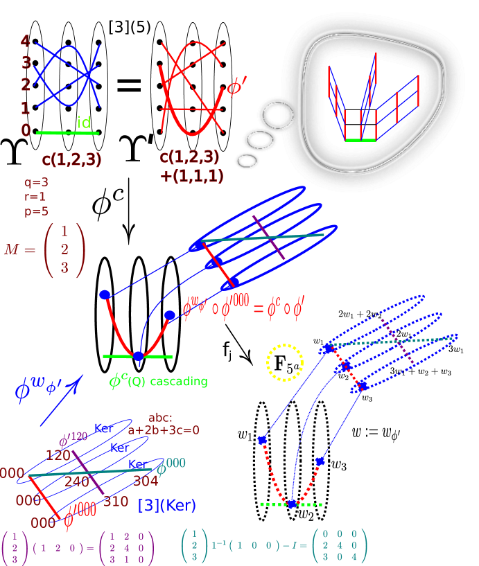
Figure 1: A cascade

We start with the ‘thought bubble’ in the top right of the picture, which contains a ‘cartoon cascade’. The blue diagonal triples represent some triples of the template. The green horizontal triple at the bottom represents the ‘target’: we want to modify the template so that it contains the green triple, without changing the set of vertices that it covers. To achieve this, we first replace the blue triples by the vertical red triples, which is valid as they are both matchings covering the same set of vertices. Then the three vertical red triples in the square can be replaced by three horizontal triples that cover the same vertices, and include the green triple, as desired.

The cartoon cascade was obtained by gluing together four copies of a simpler structure, namely a set of nine vertices with two decompositions into three triples. Three of these copies use template edges, and correspond to what we later call ‘absorbers’: these are subsets (in general subgraphs) of the template with two decompositions, one of which only uses template triples (in general $q$-cliques). The red triples in the picture correspond to cliques that we will call ‘absorbable’: these can be included in the template by ‘flipping’ the relevant absorber, with no need for a cascade.

The reader may wonder why we do not also describe the green triple as ‘absorbable’, given that it is obtained by the net result of the above replacements, which take the nine blue template triples and replace them by nine other triples that include the green one. The reason is that the algebraic structure naturally associates to any clique a simple configuration that acts as an absorber if it is present in $G$ (e.g. for triangle decompositions in [22] we associate octahedra to triangles). Thus we have a naturally defined subfamily of cliques with simple absorbers, which we combine into more complicated structures (cascades) that absorb a larger family of ‘cascading’ cliques.

In our illustration we glue three absorbers onto a ‘base’, which we chose to be isomorphic to an absorber. However, this is not necessary, and in general it will be convenient to use a different structure for the base, which is simpler than that of the absorbers.

Now we turn to the details of an actual cascade, in the case $q=3$ and $r=1$. We will use the prime $p=5$ (which is not as large as advertised elsewhere, but the construction still works). We fix the generic $3\times 1$ matrix $M=(1\ 2\ 3)^{t}$.

The top left of the picture illustrates the ‘blueprint’ for the base of the cascade, which consists of two perfect $3$-graphs matchings $\Upsilon$ and $\Upsilon^{\prime}$ on a set of $15$ points (the same set, drawn twice for clarity), divided into $3$ parts of size $5$, where each triple is transverse to the partition. Reading each triple of $\Upsilon$ or $\Upsilon^{\prime}$ as a vector, $\Upsilon$ consists of all $c(1,2,3)$ and $\Upsilon^{\prime}$ of all $c(1,2,3)+(1,1,1)$, where $c\in\mathbb{F}_{5}$.

The base of any cascade is defined by some embedding $\phi^{c}$ of this blueprint of the base in the template. Note that here ‘embedding’ only constrains the vertices (in general $r$-edges); the triples (in general $q$-cliques) are contained in the underlying graph of the template but may not belong to the template decomposition.

Similarly to the cartoon cascade, the cascade will flip in two stages. The first stage will provide absorbers for the cliques in $\Upsilon^{\prime}$, which can be flipped so that all cliques of $\Upsilon^{\prime}$ are present in the decomposition. The second stage is to flip the base, i.e. replace $\Upsilon^{\prime}$ by $\Upsilon$.

The green triple $(0,0,0)$ of $\Upsilon$ is mapped by $\phi^{c}$ to the target of the cascade. It is notationally convenient to identify $\mathbb{F}_{5}$ with $[5]$ so that $0$ is identified with $1$, and identify the vertices of the green triple with $[3]$. Recalling our notation to identify vectors with functions, the green triple is thus identified with $id_{[3]}$ (the identity map on $[3]$), so the target clique is $\phi^{c}(Q)=\phi^{c}([3])$.

We require each clique of $\Upsilon^{\prime}$ to be absorbable, so the remainder of the cascade will be defined by gluing absorbers onto these cliques. We illustrate this for the clique labelled $\phi^{\prime}$, where $\phi^{\prime}(1)=3$, $\phi^{\prime}(2)=1$, $\phi^{\prime}(3)=2$. In the centre of the figure this is the red clique, which has been drawn twice for clarity, once in the base of the cascade, and once in an absorber, where three vertices of the absorber are identified with the corresponding vertices of the base, and the absorber is otherwise vertex-disjoint from all other parts of the construction.

The blueprint for absorbers is illustrated in the bottom left of the figure. Similarly to the base of the cascade, it consists of two perfect $3$-graph matchings of the same set of points, divided into $3$ parts, so that each triple is transverse to the partition. However, now the parts have size $25$, and each is identified with the left kernel of $M$, i.e. all vectors $(a,b,c)\in\mathbb{F}_{5}^{3}$ (also written as $abc$) with $a+2b+3c=0$.

The absorbers in the cascade are defined by various embeddings of the blueprint absorber. These embeddings are specified with reference to one of the template embeddings $f_{j}:[n]\to\mathbb{F}_{p^{a}}$, where each cascade fixes some $j\in[z]$ for all of its absorbers. Each clique $\phi^{\prime}$ of $\Upsilon^{\prime}$ corresponds to some $w_{\phi^{\prime}}=f_{j}\phi^{c}\phi^{\prime}\in(\mathbb{F}_{5^{a}})^{3}$, i.e. a vector that can be identified with a function $w_{\phi^{\prime}}:[3]\to\mathbb{F}_{5^{a}}$ where each $w_{\phi^{\prime}}(i)=f_{j}(\phi^{c}(\phi^{\prime}(i)))$.

For convenient notation in the remainder of the illustration we fix $\phi^{\prime}$ and write $w:=w_{\phi^{\prime}}$. The actual absorber for $\phi^{c}\phi^{\prime}$ (the red clique in the middle of the figure) is obtained by embedding the blueprint absorber. This embedding is specified by a map $\phi^{w}=\phi^{w_{\phi^{\prime}}}$ satisfying $f_{j}\phi^{w}((i,a))=w_{i}+a\cdot w$, where $(i,a)$ denotes the copy of $a$ in the $i$th part, for any $i\in[3]$ and $a\in Ker$. We require the base embedding $\phi^{c}$ to be such that $\{w_{1},w_{2},w_{3}\}$ has full dimension (viewing $\mathbb{F}_{5^{a}}$ as a vector space over $\mathbb{F}_{5}$); it then follows that $\phi^{w}$ is injective.

To relate the red clique $\phi^{c}\phi^{\prime}$ to the embedding $\phi^{w}$, we note that each $f_{j}\phi^{c}\phi^{\prime}(i)=w_{i}+0\cdot w$, where $0=000$ is the zero vector in $\mathbb{F}_{5^{a}}$. We view triples in the blueprint absorber as $3\times 3$ matrices in which the $i$th row is the vector corresponding to the vertex chosen from the $i$th part. Thus $\phi^{c}\phi^{\prime}=\phi^{w}\phi^{\prime}{}^{0}$, where $\phi^{\prime}{}^{0}=\phi^{\prime}{}^{000}$ maps each $i\in[3]$ to $000$, and so can be viewed as the $3\times 3$ zero matrix.

The essential feature of absorbers is that they have two decompositions, one of which uses the target absorbable clique $\phi^{c}\phi^{\prime}=\phi^{w}\phi^{\prime}{}^{0}$, and the other of which is contained within the template decomposition. We can specify these decompositions in the blueprint absorber and then transfer them to the absorber via $\phi^{w}$. One decomposition consists of all triples $\phi^{\prime}{}^{a}$ with $a\in Ker$, specified in $3\times 3$ matrix form as the outer product $Ma$. Concretely, for each $a\in Ker$ the triple $\phi^{\prime}{}^{a}$ uses vertex $ia=(ia_{1},ia_{2},ia_{3})$ in part $i$ for $i\in[3]$. (This agrees with our above notation for $\phi^{\prime}{}^{0}$.) The purple clique illustrates this for $a=120$.

The other decomposition consists of all triples $\phi^{a}$ with $a\in Ker$, specified in $3\times 3$ matrix form as $\phi^{a}=M(a+e_{1})-I$, where $e_{1}=(1\ 0\ 0)$; the teal clique illustrates this for $a=000$. Note that all such triples are contained in the blueprint absorber, as $\phi^{a}M=M(a+e_{1})M-M=Me_{1}M-M=0$, so each row of $\phi^{a}$ is in $Ker$. Furthermore, as $f_{j}\phi^{w}((i,b))=w_{i}+b\cdot w$, we have $f_{j}\phi^{w}\phi^{a}=w+\phi^{a}w=w+(M(a+e_{1})-I)w=M(a+e_{1})w$, i.e. each $f_{j}\phi^{w}\phi^{a}$ is in the image of $M$, so $\phi^{w}\phi^{a}$ can be a template clique (if the activation and compatibility conditions of the template construction also hold).

6.2 Absorbers

Now we will implement the previous illustration in our general setting. The construction of absorbers will use the left kernel of $M$: let

$$Ker:=\{a\in\mathbb{F}_{p}^{q}:aM=0\}.$$

The following properties of $Ker$ are immediate from the construction of $M$, so we omit their proofs.

Lemma 6.1.

1. $\dim(Ker)=q-r$, so $|Ker|=p^{q-r}$,

2. if $a\in Ker$ with $a\neq 0$ then $|\{i:a_{i}\neq 0\}|>r$,

3. for any $I\in Q$ and $i\in[q]\setminus I$, the unique $a\in Ker$ with $a_{i}=-1$ and $a_{j}=0$ for all $j\in[q]\setminus(I\cup\{i\})$ is $a=e_{i}M_{I}^{-1}e_{I}-e_{i}$.

Given $a=(a^{i}:i\in I)$ with each $a^{i}\in\mathbb{F}_{p}^{q}$, we identify $a$ with a matrix $a\in\mathbb{F}_{p}^{I\times[q]}$ having entries $(a^{i}_{i^{\prime}}:i\in I,i^{\prime}\in[q])$. For $a\in Ker^{r}\subseteq\mathbb{F}_{p}^{[r]\times[q]}$ and $w\in\mathbb{F}_{p^{a}}^{q}$ we write

$$v^{w}_{a}=MM_{[r]}^{-1}(e_{[r]}+a)w\quad\text{ and }\quad v^{\prime}{}^{w}_{a}=w+Maw.$$

For example, if $a=0\in Ker^{r}$ then $v^{\prime}{}^{w}_{0}=w$ and $v^{w}_{0}=MM_{[r]}^{-1}w_{[r]}$ is a vector in the image of $M$ that might correspond to a template clique containing an edge that corresponds to $w_{[r]}$.

We write $[q](Ker)$ for the set of partite maps $f:[q]\to[q]\times Ker$ (i.e. each $f(i)$ is some $(i,a)$ with $a\in Ker$). Now we come to the key definition of this subsection.

Definition 6.2.

(absorbers) Suppose $\phi(Q)\subseteq G^{*}_{j}$ with $j\in[z]$ and $w:=f_{j}\phi\in\mathbb{F}_{p^{a}}^{q}$ has $\dim(w)=q$.

Suppose $\phi^{w}:[q]\times Ker\to[n]$ such that

1. $f_{j}\phi^{w}((i,a))=w_{i}+a\cdot w$ for each $i\in[q]$, $a\in Ker$,

2. if $\phi^{\prime}\in[q](Ker)$ with $f_{j}\phi^{w}\phi^{\prime}=v^{w}_{a}$ for some $a\in Ker^{r}$ then $\phi^{w}\phi^{\prime}(Q)\in M^{*}_{j}$.

We say that $\phi$ is absorbable and call $\phi^{w}$ the absorber for $\phi$.

We also call $A^{\phi(Q)}=A^{w}=\phi^{w}(K^{r}_{q}(Ker))$ the absorber for $\phi(Q)$.

The essential property of absorbers (see Lemma 6.4 below) is that they can be decomposed in two ways, one of which uses cliques that all belong to template, and the other of which uses any absorbable ‘target’ clique.

First we make some comments on the definition. The notation $A^{w}$ is ambiguous, but will be clear from the context, as $j$ in Definition 6.2 is uniquely determined by $\phi(Q)\subseteq G^{*}_{j}$. The notation $A^{\phi(Q)}$ is also ambiguous in that we could reorder $\phi$ without changing $\phi(Q)$, but the order will be clear from the context (we will only consider $\pi$-compatible $\phi$).

Next we introduce some notation for edges in absorbers. The edges of the complete $q$-partite $r$-graph $A^{w}=\phi^{w}(K^{r}_{q}(Ker))$ correspond to choices $I\in Q=\tbinom{[q]}{r}$ of $r$ parts and any choices of vertices $\phi^{w}((i,a^{i}))$ in these parts for each $i\in I$. We identify $(a^{i}:i\in I)$ with $a\in Ker^{I}$ and denote the corresponding edge by $e^{w}_{a}$. By Definition 6.2.i we have $f_{j}(e^{w}_{a})=(e_{I}+a)w$.

An easy but important property of absorbers is established by the following lemma, which shows that all edges have full dimension in their relevant embedding (so, in particular, all $w_{i}+a\cdot w$ are distinct, so $\phi^{w}$ is injective).

Lemma 6.3.

Suppose $A^{w}$ is the absorber of $Q^{\prime}\in K^{r}_{q}(G^{*}_{j})$. Then each $\dim(f_{j}(e^{w}_{a}))=r$.

Proof. Suppose $a\in Ker^{I}$ and $c\in\mathbb{F}_{p}^{r}$ with $c(e_{I}+a)w=0$. As $\dim(w)=q$ we must have $c(e_{I}+a)=0$. Then $0\neq-ce_{I}=ca\in Ker$, has at most $r$ nonzero coordinates, contradicting Lemma 6.1. $\Box$

We require some more notation to specify the clique decompositions of absorbers. We can write Definition 6.2.i as $f_{j}\phi^{w}\phi^{\prime}=w+\phi^{\prime}w$ for all $\phi^{\prime}\in[q](Ker)$, viewing $\phi^{\prime}$ as a matrix in $\mathbb{F}_{p}^{q\times q}$. For $a\in Ker^{r}$ we define $\phi^{a}$ and $\phi^{\prime}{}^{a}$ in matrix form by

$$\phi^{a}:=MM_{[r]}^{-1}(e_{[r]}+a)-I\quad\text{ and }\quad\phi^{\prime}{}^{a}=Ma.$$ (1)

Then for $\phi^{w}$ as in Definition 6.2.i we have

$$f_{j}\phi^{w}\phi^{a}=w+\phi^{a}w=v^{w}_{a}\quad\text{ and }\quad f_{j}\phi^{w}\phi^{\prime}{}^{a}=w+\phi^{\prime}{}^{a}w=v^{\prime}{}^{w}_{a}.$$

We write

$$\Psi(\phi^{w})=\{\phi^{w}\phi^{a}(Q):a\in Ker^{r}\}\quad\text{ and }\quad\Psi^{\prime}(\phi^{w})=\{\phi^{w}\phi^{\prime}{}^{a}(Q):a\in Ker^{r}\}.$$

Note that $\Psi^{\prime}(\phi^{w})$ contains the clique $\phi^{w}\phi^{\prime}{}^{0}(Q)$ with vertex set $f_{j}^{-1}(v^{\prime}{}^{w}_{0})=f_{j}^{-1}(w)=Im(\phi)$, and $\Psi(\phi^{w})\subseteq M^{*}_{j}$ by Definition 6.2.ii. Thus the following lemma shows that the absorber for $\phi(Q)$ can be used to modify the template, replacing $\Psi(\phi^{w})$ by $\Psi^{\prime}(\phi^{w})$, so that it contains $\phi(Q)$ (we say that we ‘flip’ $A^{\phi(Q)}$).

Lemma 6.4.

$\Psi(\phi^{w})$ and $\Psi^{\prime}(\phi^{w})$ are both $K^{r}_{q}$-decompositions of $A^{\phi(Q)}$.

Proof. First we claim that each clique in $\Psi(\phi^{w})$ and $\Psi^{\prime}(\phi^{w})$ intersects each part $A^{w}_{i}=f_{j}^{-1}\{w_{i}+a\cdot w:a\in Ker\}$. To see this, note that a $q$-set intersects each $A^{w}_{i}$ if and only if it can be written as $f_{j}^{-1}((I+B)w)$ for some $q\times q$ matrix $B\in Ker^{q}$. As $f_{j}\phi^{w}\phi^{\prime}{}^{a}=v^{\prime}{}^{w}_{a}=(I+Ma)w$ and $f_{j}\phi^{w}\phi^{a}=v^{w}_{a}=MM_{[r]}^{-1}(e_{[r]}+a)w$, the claim follows from $(I+Ma)M=IM=M$ and $MM_{[r]}^{-1}(e_{[r]}+a)M=MM_{[r]}^{-1}M_{[r]}=M$.

Now consider any $e^{w}_{a}\in A^{w}$, where $a\in Ker^{I}$ for some $I\in Q$. Then $e^{w}_{a}\in\phi^{w}\phi^{\prime}{}^{M_{I}^{-1}a}(Q)\in\Psi^{\prime}(\phi^{w})$, and $e^{w}_{a}\in\phi^{w}\phi^{a^{\prime}}(Q)\in\Psi(\phi^{w})$ where $e_{I}+a=M_{I}M_{[r]}^{-1}(e_{[r]}+a^{\prime})$, i.e. $a^{\prime}=M_{[r]}M_{I}^{-1}(e_{I}+a)-e_{[r]}$ (note that $a^{\prime}M=M_{[r]}M_{I}^{-1}M_{I}-M_{[r]}=0$). As $|\Psi(\phi^{w})|=|\Psi^{\prime}(\phi^{w})|=|Ker|^{r}=Q^{-1}|A^{w}|$, the lemma follows. $\Box$

6.3 Cascades

Absorbable cliques are plentiful but not ubiquitous. Here we will describe a much wider class of cliques that can be included in the template via a series of modifications using absorbable cliques.

First we describe our clique exchange tool, which will also be used in section 7 for the Clique Exchange Algorithm. It consists of two suitable decompositions of a small fixed $r$-graph: we use the complete $q$-partite $r$-graph $K^{r}_{q}(p)$ with $p$ vertices in each part.

Lemma 6.5.

There are $K^{r}_{q}$-decompositions $\Upsilon$ and $\Upsilon^{\prime}$ of $\Omega=K^{r}_{q}(p)$ such that

1. $|V(f)\cap V(f^{\prime})|\leq r$ for all $f\in\Upsilon$ and $f^{\prime}\in\Upsilon^{\prime}$,

2. if $f\in\Upsilon$ and $\{f^{\prime},f^{\prime\prime}\}\subseteq\Upsilon^{\prime}$ with $|V(f)\cap V(f^{\prime})|=|V(f)\cap V(f^{\prime\prime})|=r$

   then $(V(f^{\prime})\setminus V(f))\cap(V(f^{\prime\prime})\setminus V(f))=\emptyset$.

The construction requires a matrix of the same type as that used in constructing the template, with an additional technical property.

Definition 6.6.

Let $M^{\prime}\in\mathbb{F}_{p}^{q\times r}$ be such that every square submatrix of $M^{\prime}$ is nonsingular and for any $r\times r$ submatrix $A$ of $M^{\prime}$ and row $v$ of $M^{\prime}$ not in $A$ each entry of $vA^{-1}$ is not $0$ or $1$.

To see that such $M^{\prime}$ exists we again consider a uniform random $M^{\prime}$, and recall from the construction of $M$ that the probability of having any singular square submatrix is at most $2^{q+r+1}p^{-1}$. Now fix any $r\times r$ submatrix $A$ of $M^{\prime}$ and row $v$ of $M^{\prime}$ not in $A$: there are fewer than $q2^{q}$ choices. There are fewer than $2rp^{r-1}$ row vectors $w\in\mathbb{F}_{p}^{r}$ such that some entry is $0$ or $1$. We fix any such $w$ and bound $\mathbb{P}(Aw=v)$. We can assume $w\neq 0$, as otherwise $v=0$, so $M^{\prime}$ has zero entries, which are singular $1$ by $1$ submatrices. Without loss of generality $w_{1}\neq 0$. We condition on any value of $v$ and all but the first column of $A$. Then $Aw$ is uniformly random, so $\mathbb{P}(Aw=v)=p^{-r}$. Thus the required properties of $M^{\prime}$ fail with probability at most $2^{q+r+1}p^{-1}+2rq2^{q}p^{-1}<1$, so $M^{\prime}$ exists.

Proof of Lemma 6.5. We identify each part $\Omega_{i}$ of $\Omega$ with $\mathbb{F}_{p}$. We let $\Upsilon$ consist of all $q$-cliques $Q^{\prime}$ of the form $M^{\prime}x$, i.e. for some $x\in\mathbb{F}_{p}^{r}$ we have $V(Q^{\prime})\cap\Omega_{i}=(M^{\prime}x)_{i}$ for all $i\in[q]$. We choose $c\in(\mathbb{F}_{p}\setminus\{0\})^{q}$ uniformly at random and let $\Upsilon^{\prime}$ consist of all $q$-cliques $Q^{\prime}$ of the form $M^{\prime}x+c$.

Now for any $I\in Q$ and $z_{I}\in\mathbb{F}_{p}^{I}$, there is a unique $q$-clique $v=M^{\prime}(M^{\prime}_{I})^{-1}z_{I}$ in $\Upsilon$ containing $z_{I}$, and a unique $q$-clique $v^{\prime}=M^{\prime}(M^{\prime}_{I})^{-1}(z_{I}-c_{I})+c$ in $\Upsilon^{\prime}$ containing $z_{I}$. Thus $\Upsilon$ and $\Upsilon^{\prime}$ are $K^{r}_{q}$-decompositions of $\Omega$.

To show properties (i) and (ii) we show that the failure of each corresponds to a nontrivial linear equation in $c$, so with positive probability there is some $c$ such that (i) and (ii) hold.

If property (i) failed we would have $i\notin I\in Q$ with $c_{i}=M^{\prime}_{i}(M^{\prime}_{I})^{-1}c_{I}$, which is an equation for $c$ with a nonzero coefficient of $c_{i}$ by construction of $M^{\prime}$ (no entry of $M^{\prime}_{i}(M^{\prime}_{I})^{-1}$ is equal to $1$).

If property (ii) failed we would have $\{I,I^{\prime}\}\subseteq Q$ and $i\notin I\cup I^{\prime}$ with $M^{\prime}_{i}(M^{\prime}_{I})^{-1}c_{I}=M^{\prime}_{i}(M^{\prime}_{I^{\prime}})^{-1}c_{I^{\prime}}$. We can choose $i^{\prime}\in I\setminus I^{\prime}$, and then $c_{i^{\prime}}$ appears with nonzero coefficient in the equation (no coefficient of $M^{\prime}_{i}(M^{\prime}_{I})^{-1}$ is equal to $0$).

This gives at most $qQ+Q^{2}$ equations for $c$, each holding with probability at most $(p-1)^{-1}$, so we can choose $c$ such that (i) and (ii) hold. $\Box$

We identify $\Upsilon$ and $\Upsilon^{\prime}$ with subsets of $[q](p)$, i.e. the set of partite maps from $[q]$ to $[q]\times[p]$. We identify $[q]$ with $\{(i,1):i\in[q]\}\subseteq V(\Omega)$ and with the corresponding map $id_{[q]}$; by relabelling we can assume $[q]\in\Upsilon$. Next we require some more terminology.

Definition 6.7.

Suppose $U^{\prime}\subseteq U\subseteq[n]$. We say that $U$ is $j$-generic for $U^{\prime}$ if $\dim(f_{j}(U))=\dim(f_{j}(U^{\prime}))+|U|-|U^{\prime}|$. We say that $U$ is generic for $U^{\prime}$ if $U$ is $j$-generic for $U^{\prime}$ for all $j\in[z]$.

Note that given $U^{\prime}\in\tbinom{[n]}{u^{\prime}}$, all but $O(n^{u-u^{\prime}-1})$ sets $U\in\tbinom{[n]}{u}$ containing $U^{\prime}$ are generic for $U^{\prime}$. Now we can give the key definition of this subsection.

Definition 6.8.

(cascades) Suppose $Q^{\prime}=\phi(Q)\subseteq G^{*}_{j}$ and $\phi^{c}$ is an embedding of $K^{r}_{q}(p)$ in $G^{*}_{j}$ where $\phi^{c}id_{[q]}=\phi$ and $Im(\phi^{c})$ is $j$-generic for $Im(\phi)$, such that each $\phi^{c}\phi^{\prime}$ with $\phi^{\prime}\in\Upsilon^{\prime}$ is absorbable, with absorber $A^{\phi^{c}\phi^{\prime}(Q)}=\phi^{w_{\phi^{\prime}}}(K^{r}_{q}(Ker))$, and $C_{\phi^{c}}=\sum\{A^{\phi^{c}\phi^{\prime}(Q)}:\phi^{\prime}\in\Upsilon^{\prime}\}$ is a set (without multiple elements). We call $C_{\phi^{c}}$ a cascade for $Q^{\prime}$.

A cascade for $Q^{\prime}$ provides a two-step process for modifying the template so as to include $Q^{\prime}$: we flip all of the absorbers in the cascade, and then flip the $K^{r}_{q}$-decomposition of the base embedding of $\Omega$. Formally, to flip a cascade $C_{\phi^{c}}$ we replace

$$\Psi(C_{\phi^{c}}):=\bigcup\{\Psi(w_{\phi^{\prime}}):\phi^{\prime}\in\Upsilon^{\prime}\}\qquad\text{ by }$$

$$\Psi^{\prime}(C_{\phi^{c}}):=\{\phi^{c}\phi^{\prime}(Q):\phi^{\prime}\in\Upsilon\}\cup\bigcup\{\Psi^{\prime}(w_{\phi^{\prime}})\setminus\{\phi^{c}\phi^{\prime}(Q)\}:\phi^{\prime}\in\Upsilon^{\prime}\}.$$

This has the desired property as $\phi(Q)=\phi^{c}(Q)\in\Psi^{\prime}(C_{\phi^{c}})$. Next we define the set of cliques for which we will show (Lemma 6.15) that we have many cascades.

Definition 6.9.

(cascading cliques) Let $\mathcal{Q}^{*}=\cup_{j\in[z]}\mathcal{Q}_{j}$, where each $\mathcal{Q}_{j}$ is the set of all $\phi(Q)\subseteq G^{*}_{j}$ where $\phi$ is $\pi$-compatible and $\dim(f_{j}\phi)=q$.

In analysing the choice of cascades, we will often need to know how fixing the image of one edge constrains the possible images of some other edge. We will define bipartite graphs $B^{aI^{\prime}}_{j\phi^{\prime}}$ describing which pairs of edges $(e,e^{\prime})$ in some $G^{*}_{j}$ can satisfy $e=e^{w_{\phi^{\prime}}}_{a}$ and $e^{\prime}=\phi^{c}(I^{\prime})$. In the accompanying lemma we show that $f_{j}$ embeds $B^{aI^{\prime}}_{j\phi^{\prime}}$ in an algebraically defined regular bipartite graph $AB^{aI^{\prime}}_{J}$, for which we can describe neighbourhoods as certain affine linear spaces, all of the same dimension.

Definition 6.10.

(cascade edge compatibility graphs)

Let $\phi^{\prime}\in\Upsilon^{\prime}$ and $J\subseteq I^{\prime}\in Q$ where $J=\{i\in[q]:\phi^{\prime}(i)=(i,1)=i\}$. Let $a\in Ker^{I}$ with $I\in Q$.

Let $B^{aI^{\prime}}_{j\phi^{\prime}}\subseteq G^{*}_{j}\times G^{*}_{j}$ be the bipartite graph where $(e,e^{\prime})$ is an edge if there is a cascade $C_{\phi^{c}}$ for some $Q^{\prime}=\phi^{c}([q])$ with $\phi^{c}(I^{\prime})=e^{\prime}$ where $A^{\phi^{c}\phi^{\prime}(Q)}=\phi^{w_{\phi^{\prime}}}(K^{r}_{q}(Ker))$ with $e=e^{w_{\phi^{\prime}}}_{a}$.

Let $AB^{aI^{\prime}}_{J}\subseteq\mathbb{F}_{p^{a}}^{I}\times\mathbb{F}_{p^{a}}^{I^{\prime}}$ be the bipartite graph where $(x,x^{\prime})$ is an edge if there is a solution $w\in\mathbb{F}_{p}^{q}$ to the simultaneous equations $w_{i}+a_{i}\cdot w=x_{i}$ for $i\in I$ and $w_{i}=x^{\prime}_{i}$ for $i\in J$.

We let $r_{a\phi^{\prime}}=\operatorname{rank}Y$ where $Y=(e_{I}+a)e_{[q]\setminus J}^{T}$.

Lemma 6.11.

With notation as in Definition 6.10,

1. if $(e,e^{\prime})\in B^{aI^{\prime}}_{j\phi^{\prime}}$ then $(f_{j}(e),f_{j}(e^{\prime}))\in AB^{aI^{\prime}}_{J}$, regarded in $\mathbb{F}_{p^{a}}^{I}\times\mathbb{F}_{p^{a}}^{I^{\prime}}$ via $(\pi_{e},\pi_{e^{\prime}})$,

2. every vertex neighbourhood in $AB^{aI^{\prime}}_{J}$ is an affine linear space of dimension $r_{a\phi^{\prime}}$.

Here (and later) we require the following easy fact from linear algebra (we omit the proof).

Lemma 6.12.

Let $\mathbb{F}$ be a field, $A\in\mathbb{F}^{a\times q}$, $B\in\mathbb{F}^{b\times q}$ and $c\in\{Bw:w\in\mathbb{F}^{q}\}$. Then $\{Aw:Bw=c\}$ is an affine linear space of dimension $\operatorname{rank}\tbinom{A}{B}-\operatorname{rank}B$.

Proof of Lemma 6.11.

To see (i), note that if $e=e^{w}_{a}$ with $w=w_{\phi^{\prime}}$ then $f_{j}(e)=(e_{I}+a)w$, which has $i$-coordinate $w_{i}+a_{i}\cdot w$ for each $i\in I$, and if $\phi^{c}(I^{\prime})=e^{\prime}$ then $f_{j}\phi^{c}(i)=w_{i}$ for each $i\in J$.

For (ii), we write $e_{I}+a=(X\ Y)$ where $X=(e_{I}+a)e_{J}^{T}$ and $Y=(e_{I}+a)e_{[q]\setminus J}^{T}$, i.e. $X$ contains the columns indexed by $J$ and $Y$ those indexed by $[q]\setminus J$.

Consider any $x^{\prime}\in\mathbb{F}_{p^{a}}^{I^{\prime}}$. If $(x,x^{\prime})$ is an edge with some solution $w$ then we can write $x=(e_{I}+a)w=Xw_{J}+Yw_{[q]\setminus J}=Xx^{\prime}_{J}+Yw_{[q]\setminus J}$, so $x$ must lie in the affine space $Xx^{\prime}_{J}+\text{Im}(Y)$.

Now consider any $x\in\mathbb{F}_{p^{a}}^{I}$. In choosing $x^{\prime}\in\mathbb{F}_{p^{a}}^{I^{\prime}}$, the coordinates $x^{\prime}_{i}$ with $i\in I^{\prime}\setminus J$ are unconstrained, whereas those in $J$ satisfy $x^{\prime}_{J}\in\{e_{J}w:(e_{I}+a)w=x\}$. By Lemma 6.3, $x^{\prime}$ lies in an affine space $W$ with $\dim(W)=r-|J|+\operatorname{rank}Z-\operatorname{rank}(e_{I}+a)$, where $Z=\bigl{(}\begin{smallmatrix}e_{J}&0\\ X&Y\end{smallmatrix}\bigr{)}$. Note that $Z$ is row-equivalent to $\bigl{(}\begin{smallmatrix}e_{J}&0\\ 0&Y\end{smallmatrix}\bigr{)}$, so has rank $|J|+r_{a\phi^{\prime}}$, and $e_{I}+a$ has rank $r$ by Lemma 6.3. Thus $\dim(W)=r-|J|+|J|+r_{a\phi^{\prime}}-r=r_{a\phi^{\prime}}$, as required. $\Box$

Remark 6.13.

We will only ever consider $\phi^{\prime}$ and $a$ as in Definition 6.10 such that setting $e=e^{w_{\phi^{\prime}}}_{a}$ and $e^{\prime}=\phi^{c}(I^{\prime})$ does not imply that $e$ and $e^{\prime}$ belong to the same clique of the template $M^{*}$. This condition is equivalent to $r_{a\phi^{\prime}}>0$, i.e. $Y=(e_{I}+a)e_{[q]\setminus J}^{T}\neq 0$. To see this, we note for any $i\in I$ that if row $i$ of $Y$ is $0$ then $1_{i=j}+a_{ij}=0$ for all $j\in[q]\setminus J$, which by Lemma 6.1.iii implies $i\notin J=I^{\prime}\in Q$ and $a_{i}=e_{i}MM_{I^{\prime}}^{-1}-e_{i}$. However, if this holds for all $i\in I$ then $e^{\prime}=\phi^{c}(I^{\prime})$ and $e=e^{w_{\phi^{\prime}}}_{a}$ imply that $e$ is the $I$-edge of $M^{*}(e^{\prime})$.

The proof of concentration in Lemma 6.15 uses the following upper bound on the number of cascades for a given clique using a given edge; this bound will also be used in the analysis of the cascade algorithm in the proof of Theorem 1.10.

Lemma 6.14.

Suppose $Q^{\prime}=\phi(Q)\in\mathcal{Q}_{j}$ and $e\in G^{*}$. Let $\phi^{\prime}\in\Upsilon^{\prime}$, $I\in Q$, $a\in Ker^{I}$. Then there are at most $(p^{a})^{q(p-1)-r_{a\phi^{\prime}}}$ cascades $C_{\phi^{c}}$ for $Q^{\prime}$ such that the absorber $A^{\phi^{c}\phi^{\prime}(Q)}=\phi^{w_{\phi^{\prime}}}(K^{r}_{q}(Ker))$ for $\phi^{c}\phi^{\prime}$ satisfies $e^{w_{\phi^{\prime}}}_{a}=e$.

Proof. Any cascade $C_{\phi^{c}}$ for $Q^{\prime}$ determines some $w^{C}=f^{j}\phi^{c}\in\mathbb{F}_{p^{a}}^{[q]\times[p]}$ with $w^{\prime}:=w^{C}_{[q]}=f_{j}\phi$, and any such $w^{C}$ corresponds to at most one cascade for $Q^{\prime}$. The condition $e^{w_{\phi^{\prime}}}_{a}=e$ imposes the additional constraint $(e_{I}+a)w=b$, where $w:=f_{j}\phi^{c}\phi^{\prime}$ and $b:=f_{j}(e)$ (regarded in $\mathbb{F}_{p^{a}}^{I}$ via $\pi_{e}$). Let $J=\{i\in[q]:\phi^{\prime}(i)=i\}$. Noting that $w^{\prime}_{J}=w_{J}$, we write $w^{C}=(w^{C^{\prime}},w^{\prime}_{[q]\setminus J},w)$, and apply Lemma 6.12 to see that the choices for $w^{C}$ lie in an affine space $W$ with $\dim W=\operatorname{rank}\tbinom{A}{B}-\operatorname{rank}B$, where $A=I_{pq}$ (an identity matrix) and $B=\Big{(}\begin{smallmatrix}0&0&0\\ 0&I_{q-|J|}&0\\ 0&0&Z\end{smallmatrix}\Big{)}$, with $Z$ as in the proof of Lemma 6.11. Recalling that $\operatorname{rank}Z=|J|+r_{a\phi^{\prime}}$, we have $\dim W=pq-(q-|J|+|J|+r_{a\phi^{\prime}})=q(p-1)-r_{a\phi^{\prime}}$. $\Box$

Now we give a lower bound on the number of cascades on any cascading clique (to see that it is effective recall $p^{q^{2}}<2^{9q^{3}}<h^{1/5}$ and $\omega>n^{-b^{-1}h^{-2}}$).

Lemma 6.15.

For any $Q^{\prime}=\phi(Q)\in\mathcal{Q}_{j}$ there are at least $\omega^{p^{q^{2}}}n^{q(p-1)}$ cascades for $Q^{\prime}$.

Proof. We condition on local events $\mathcal{E}=\cap_{e\in Q^{\prime}}\mathcal{E}^{e}$ such that $Q^{\prime}\in\mathcal{Q}_{j}$. Then $\dim(f_{j}\phi)=q$ and $\phi$ is $\pi$-compatible, so for each $e\in\phi(Q)$ we can write $M^{*}(e)=\phi^{e}(Q)$ with $\pi_{e}\phi^{e}=\pi_{e}\phi=id$. Let $U$ be the set of vertices touched by $\mathcal{E}$.

Now we consider any fixed combinatorial structure that could be a cascade for $Q^{\prime}$ if it satisfies the necessary algebraic constraints. We fix any embedding $\phi^{c}$ of $K^{r}_{q}(p)$ in $G$ with $\phi^{c}id_{[q]}=\phi$ and $Im(\phi^{c})\setminus Im(\phi)$ disjoint from $U$; recalling the illustration above, this specifies the base of the cascade, and $\phi(Q)=\phi^{c}(Q)$ is represented by the green clique in Figure 1.

We also need to specify the combinatorial structure of the absorbers. For each $\phi^{\prime}\in\Upsilon^{\prime}$ we fix any embedding $\phi^{\phi^{\prime}}$ of $K^{r}_{q}(Ker)$ in $G$ with $\phi^{\phi^{\prime}}\phi^{\prime}{}^{0}=\phi^{c}\phi^{\prime}$, recalling that $\phi^{\prime}{}^{0}=(0,\dots,0)$ is identified with $[q]$; this is illustrated by the red clique $\phi^{c}\phi^{\prime}(Q)$ in Figure 1 (we will add algebraic constraints below so that $\phi^{w_{\phi^{\prime}}}=\phi^{\phi^{\prime}}$).

There is an additional constraint on $\phi^{\phi^{\prime}}$ for each $\phi^{\prime}\in\Upsilon^{\prime}$ with $|Im(\phi^{\prime})\cap[q]|=r$. Indeed, then the red clique $\phi^{c}\phi^{\prime}(Q)$ shares an edge with the green clique $\phi(Q)=\phi^{c}(Q)$; such a $\phi^{\prime}$ is illustrated in Figure 1 (where $r=1$, so an ‘edge’ is a vertex). If this edge is $e\in\phi(Q)$ we denote $\phi^{\prime}$ by $\phi^{\prime}_{e}$. The absorber for $\phi^{c}\phi^{\prime}_{e}(Q)$ must contain the template clique $M^{*}(e)$ which contains $e$. Accordingly, for each $e\in\phi(Q)$ we let $a_{e}\in Ker^{r}$ be such that $Im(\pi_{e})\subseteq Im(\phi^{a_{e}})$, where we identify $[q]$ with $[q]\times\{0\}\subseteq[q]\times Ker$ and recall $\phi^{a_{e}}$ from (1). Then $\phi^{a_{e}}$ must correspond to the template clique containing $e$, so we require $\phi^{\phi^{\prime}_{e}}\phi^{a_{e}}=\phi^{e}$.

The final combinatorial condition on the cascade is that the base and absorbers should be ‘as disjoint as possible’ subject to the gluing of the absorbers onto the base. For each $\phi^{\prime}\in\Upsilon^{\prime}$, the set of ‘private’ vertices of the absorber for $\phi^{c}\phi^{\prime}$ is $I_{\phi^{\prime}}=Im(\phi^{\phi^{\prime}})\setminus Im(\phi^{c}\phi^{\prime})$ if $\phi^{\prime}$ is not some $\phi^{\prime}_{e}$, or $I_{\phi^{\prime}_{e}}=Im(\phi^{\phi^{\prime}_{e}})\setminus(Im(\phi^{c}\phi^{\prime}_{e})\cup Im(\phi^{e}))$. We choose the $\phi^{\phi^{\prime}}$ so that the $I_{\phi^{\prime}}$ are pairwise disjoint and disjoint from $U\cup Im(\phi^{c})$. This is possible for $I_{\phi^{\prime}_{e}}$ by Lemma 6.5.ii as $\dim(f_{j}\phi)=q$ so $Im(\phi^{e})\setminus e$ are pairwise disjoint for all $e\in\phi(Q)$.

As $G$ is $(\omega,h)$-extendable, the number of such choices for $\phi^{c}$ and $\phi^{\phi^{\prime}}$ given $\phi$ and $\mathcal{E}$ is at least $0.9\omega n^{q(p-1)+v_{+}}$, where $v_{+}=\sum_{\phi^{\prime}}|I_{\phi^{\prime}}|=p^{r}q(p^{q-r}-1)-Q(q-r)$.

Next we specify the algebraic constraints. We condition on $f_{j}\phi^{c}$ such that $Im(\phi^{c})$ is $j$-generic for $Im(\phi)$, which occurs with probability $1-O(n^{-1})$. We define $w_{\phi^{\prime}}=f_{j}\phi^{c}\phi^{\prime}$ for $\phi^{\prime}\in\Upsilon^{\prime}$ and note that each $\dim(w_{\phi^{\prime}})=q$, as $Im(\phi^{c})$ is $j$-generic for $Im(\phi)$ and $\dim(f_{j}\phi)=q$ as $Q^{\prime}=\phi(Q)\in\mathcal{Q}_{j}$.

Then $\phi^{c}$ will define a cascade $C_{\phi^{c}}=\sum\{A^{\phi^{c}\phi^{\prime}(Q)}:\phi^{\prime}\in\Upsilon^{\prime}\}$ with each $A^{\phi^{c}\phi^{\prime}(Q)}=\phi^{w_{\phi^{\prime}}}(K^{r}_{q}(Ker))=\phi^{\phi^{\prime}}(K^{r}_{q}(Ker))$ as in Definitions 6.2 and 6.8 if

1. $f_{j}\phi^{\phi^{\prime}}((i,a))=(w_{\phi^{\prime}})_{i}+a\cdot w_{\phi^{\prime}}$ for each $\phi^{\prime}\in\Upsilon^{\prime}$, $i\in[q]$, $a\in Ker$, and

2. $\phi^{\phi^{\prime}}\phi^{a}(Q)$ is activated and $T_{e}=j$ and $\pi_{e}\phi^{\phi^{\prime}}\phi^{a}=id$ for all $\phi^{\prime}\in\Upsilon^{\prime}$, $a\in Ker^{r}$, $e\in\phi^{\phi^{\prime}}\phi^{a}(Q)$.

Given $f_{j}\phi^{c}$, as all cliques are activated independently with probability at least $\omega^{2}$, these events occur with probability $(1+O(n^{-1}))(p^{-a})^{v_{+}}((z(q)_{r})^{-Q}\omega^{2})^{p^{r(q-r+1)}}$, provided that (i) does not contradict injectivity of $f_{j}$: we need to show that $(w_{\phi^{\prime}})_{i}+a\cdot w_{\phi^{\prime}}$ are distinct for distinct choices of $(\phi^{\prime},i,a)$ with $\phi^{\prime}\in\Upsilon^{\prime}$, $i\in[q]$, $a\in Ker\setminus\{0\}$.

Suppose for a contradiction that we have some identity $(w_{\phi^{1}})_{i^{1}}+a^{1}\cdot(w_{\phi^{1}})=(w_{\phi^{2}})_{i^{2}}+a^{2}\cdot(w_{\phi^{2}})$. If $\phi^{1}=\phi^{2}$ then as $\dim(w_{\phi^{1}})=q$ we have $e_{i^{1}}-e_{i^{2}}=a^{1}-a^{2}\in Ker$, so $i^{1}=i^{2}$ by Lemma 6.1, so $a^{1}=a^{2}$. If $\phi^{1}\neq\phi^{2}$ then as $|\{i:a^{2}_{i}\neq 0\}|>r$ by Lemma 6.1 we can find $i\in[q]$ with $a^{2}_{i}\neq 0$ and $\phi^{2}(i)\notin Im(\phi^{1})$. Then $(w_{\phi^{2}})_{i}=f_{j}\phi^{c}\phi^{2}(i)$ appears with a nonzero coefficient in the identity but is not in the span of $w_{\phi^{1}}$ and the other coordinates of $w_{\phi^{2}}$, which gives the required contradiction.

We deduce (using $\omega<\omega_{0}$) that the number $X$ of cascades for $Q^{\prime}$ satisfies

$$\mathbb{E}[X\mid\mathcal{E}]>0.9\omega n^{q(p-1)+v_{+}}\cdot(1+O(n^{-1}))(p^{-a})^{v_{+}}((z(q)_{r})^{-Q}\omega^{2})^{p^{r(q-r+1)}}>3\omega^{p^{q^{2}}}n^{q(p-1)}.$$

For concentration of $X\mid\mathcal{E}$ we will apply Lemma 2.11 similarly to subsection 4.1. We start by showing concentration of $\mathbb{E}[X\mid\mathcal{E},f_{j}]$, i.e. the conditional expectation where we reveal the embedding $f_{j}$ but not the other random choices in the construction of the template. We claim that changing any $f_{j}(x)$ with $x\notin U$ from $\alpha$ to $\alpha^{\prime}$ affects $X$ by $O(n^{q(p-1)-1})$. To see this, it suffices to show for any $\phi^{\prime}\in\Upsilon^{\prime}$, $i\in[q]$, $a\in Ker$, writing $w=w_{\phi^{\prime}}$, that if the constraint $w_{i}+a\cdot w=\alpha$ can affect $X$ then it defines a strict subspace of the cascade variables $f_{j}\phi^{c}\setminus f_{j}\phi\in\mathbb{F}_{p^{a}}^{[q]\times[2,p]}$. We need to show that the constraint is non-trivial, in that it has a non-zero coefficient of some variable in $f_{j}\phi^{c}\setminus f_{j}\phi$. If $a=0$ then $w_{i}$ is such a variable, as the constraint can only affect $X$ when $\phi^{\prime}(i)\neq i$. If $a\neq 0$ then Lemma 6.1.iii implies that if the constraint only depends on $f_{j}\phi$ then it has the form $f_{j}(x)=\alpha$ for some $x\in U$, but we have already conditioned on this. This proves the claim. Thus $\mathbb{E}[X\mid\mathcal{E},f_{j}]$ is $O(n^{2q(p-1)-1})$-varying (in the choice of $f_{j}$), so whp $\mathbb{E}[X\mid\mathcal{E},f_{j}]>2\omega^{p^{q^{2}}}n^{q(p-1)}$ by Lemma 2.11.

Now we fix $f_{j}$ with $\mathbb{E}[X\mid\mathcal{E},f_{j}]>2\omega^{p^{q^{2}}}n^{q(p-1)}$ and show concentration of $X$ under the remaining random choices. Consider any clique $\phi^{*}(Q)\in K^{r}_{q}(G)$ such that there is some $y\in\mathbb{F}_{p^{a}}^{r}$ with $f_{j}(\phi^{*}(i))=(My)_{i}$ for all $i\in[q]$. The random choices of any $T_{e}$ or $\pi_{e}$ for $e\in\phi^{*}(Q)$ or whether $\phi^{*}(Q)$ is activated can affect whether $\phi^{*}(Q)$ is in the template, and so all cascades containing $\phi^{*}(Q)$. We consider the separately the effect according to the role of $\phi^{*}(Q)$ in the cascade: we fix $\phi^{\prime}\in\Upsilon^{\prime}$, $I\in Q$, $a\in Ker^{I}$, where we can assume $r_{a\phi^{\prime}}>0$ by Remark 6.13, and consider cascades where $\phi^{*}(Q)$ is the template clique containing $e^{w}_{a}$, where $w=w_{\phi^{\prime}}$, i.e. $f_{j}\phi^{*}=MM_{I}^{-1}(e_{I}+a)w$. By Lemma 6.11, there are at most $(p^{a})^{r_{a\phi^{\prime}}}$ choices of $e^{w}_{a}$, which determines $\phi^{*}(Q)$, and by Lemma 6.14 there are at most $(p^{a})^{q(p-1)-r_{a\phi^{\prime}}}$ cascades with $\phi^{*}(Q)$ in this role. Summing over all $\phi^{\prime}$ and $a$ we see that $X\mid\mathcal{E},f_{j}$ is $O(n^{2q(p-1)-1})$-varying, so by Lemma 2.11 whp $X>\omega^{p^{q^{2}}}n^{q(p-1)}$. $\Box$

6.4 Cascading extensions

The Clique Exchange Algorithm in section 7 will use the clique exchange tool from Lemma 6.5 and terminate with a set of signed cliques in which all positive cliques are cascading. Here we establish the lower bounds on the corresponding extensions required for the analysis of the algorithm. Throughout we use the same notation as in Lemma 6.5.

Definition 6.16.

Consider any extension $E(\phi)=(\phi,[q],\Omega)$ where $\Omega=K^{r}_{q}(p)$ and $\phi(Q)\in K^{r}_{q}(K^{r}_{n})$.

We let $X^{\pi}_{E(\phi)}(G^{*})$ be the set or number of rainbow extensions $\phi^{+}\in X^{\prime}_{E(\phi)}(G^{*})$ (recall Remark 3.9) such that each $\phi^{+}\phi^{\prime}(Q)$ with $\phi^{\prime}\in\Upsilon^{\prime}$ is $\pi$-compatible, i.e. we can order it as $\phi^{+}\phi^{\prime}(Q)=\psi(Q)$ for some $\psi$ such that $\pi_{e}\psi=id$ for all $e\in\psi(Q)$ (recall $\pi_{e}$ was defined for all $e\in K^{r}_{n}$).

We let $X^{c}_{E(\phi)}(G^{*})$ be the set or number of $\phi^{+}\in X_{E(\phi)}(G^{*})$ that are ‘rainbow $\Upsilon^{\prime}$ cascading’, i.e. $\phi^{+}\psi(Q)\in\mathcal{Q}^{*}$ (recall Definition 6.9) for all $\psi\in\Upsilon^{\prime}$, and $j\neq j^{\prime}$ whenever $\{\psi,\psi^{\prime}\}\subseteq\Upsilon^{\prime}$ with $\phi^{+}\psi(Q)\in\mathcal{Q}_{j}$, $\phi^{+}\psi^{\prime}(Q)\in\mathcal{Q}_{j^{\prime}}$.

By Lemma 3.8 and Remark 3.9 whp

$$X^{\pi}_{E(\phi)}(G^{*})>\omega n^{pq-q}(z\rho/2(q)_{r})^{Qp^{r}};$$ (2)

this estimate will be used in the Splitting Phase of the algorithm. The next estimate will be used in the Solo Phase of the algorithm.

Lemma 6.17.

If $\phi(Q)\subseteq G^{*}$ is rainbow and $\phi$ is $\pi$-compatible then whp

$$X^{c}_{E(\phi)}(G^{*})>0.9\omega^{3Q^{2}p^{r}}n^{pq-q}.$$

The proof of Lemma 6.17 requires the following analogue of Lemma 3.6.

Lemma 6.18.

Let $S\subseteq G$ with $|S|<h$ and $\mathcal{E}=\cap_{f\in S}\mathcal{E}^{f}$. Suppose $\phi(Q)\subseteq G$ has at most one edge in $S$ and the edges of $\phi(Q)\setminus S$ are not touched by $\mathcal{E}$. Let $j\in[z]$ be such that the set $R$ of $v\in\phi([q])$ such that $f_{j}(v)$ is revealed by $\mathcal{E}$ has $|R|\leq r$ and $\dim f_{j}(R)=|R|$. If $|R|=r$ suppose also that $R=e\in G^{*}_{j}$ with $\pi_{e}\phi=id$ and $\phi(Q)\cap S=\{e\}$. Then $\mathbb{P}(\phi(Q)\in\mathcal{Q}_{j}\mid\mathcal{E})>\omega^{3Q^{2}}$.

Proof. Let $1_{e}$ be $1$ if $\phi(Q)\cap S=\{e\}$ or $0$ otherwise. For $e^{\prime}\in\phi(Q)\setminus S$ let $\pi^{0}_{e^{\prime}}:e^{\prime}\to[q]$ be such that $\pi^{0}_{e^{\prime}}\phi=id$. For each $e^{\prime}\in\phi(Q)\setminus S$ we fix $\phi^{e^{\prime}}(Q)\in K^{r}_{q}(G)$ with $\pi^{0}_{e^{\prime}}\phi^{e^{\prime}}=id$ and estimate the probability that all such $e^{\prime}\in G^{*}_{j}$ with $M^{*}(e^{\prime})=\phi^{e^{\prime}}(Q)$. As $G$ is $(\omega,h)$-extendable, there are at least $(1-O(n^{-1}))\omega n^{(Q-1_{e})(q-r)}$ choices for all $\phi^{e^{\prime}}$ such that the sets $Im(\phi^{e^{\prime}})\setminus e^{\prime}$ are pairwise disjoint and disjoint from $Im(\phi)$, and no edge of any $\phi^{e^{\prime}}(Q)$ is touched by $\mathcal{E}$. The probability that $\phi^{e^{\prime}}(Q)$ is activated, $T_{f}=j$ and $\pi_{f}\phi^{e^{\prime}}=id$ for all such $e^{\prime}$ and $f\in\phi^{e^{\prime}}(Q)$ is at least $((z(q)_{r})^{-Q}\omega^{2})^{Q-1_{e}}$.

As $M$ is generic, when we reveal $f_{j}\!\mid_{Im(\phi)\setminus R}$ then each $e^{\prime}\in\phi(Q)\setminus S$ will have a unique $y^{e^{\prime}}\in\mathbb{F}_{p^{a}}^{r}$ such that $(My^{e^{\prime}})_{i}=f_{j}\pi_{e^{\prime}}^{-1}(i)$ for all $i\in Im(\pi_{e^{\prime}})$. We claim that with probability $1-O(n^{-1})$ the choice of $f_{j}\!\mid_{Im(\phi)\setminus R}$ is such that its entries and all $(My^{e^{\prime}})_{i}$ with $e^{\prime}\in\phi(Q)\setminus S$ and $i\in[q]\setminus\pi_{e^{\prime}}(e^{\prime})$ are distinct and not equal to any $f_{j}(x)$ revealed by $\mathcal{E}$. To see this, first note that there are at most $hr$ such revealed $f_{j}(x)$, and each $(My^{e^{\prime}})_{i}$ is a non-trivial linear function of the entries of $f_{j}\!\mid_{Im(\phi)\setminus R}$, so is a revealed value with probability $O(1/n)$. Also, with probability $1-O(n^{-1})$ we have $\dim(f_{j}\phi)=q$, which implies the distinctness property, so the claim holds.

With probability $(1+O(n^{-1}))(p^{-a})^{(q-r)(Q-1_{e})}$ we have $f_{j}(\phi^{e^{\prime}}(i))=(My^{e^{\prime}})_{i}$ for all such $e^{\prime}$ and $i\in[q]\setminus Im(\pi_{e^{\prime}})$. Therefore $\mathbb{P}(\cap_{e^{\prime}}\{M^{*}(e^{\prime})=\phi^{e^{\prime}}(Q)\}\mid\mathcal{E})>(1+O(n^{-1}))[(z(q)_{r}\omega^{-2})^{Q}p^{a(q-r)}]^{1_{e}-Q}$. Summing over all choices for $\phi^{e^{\prime}}$ gives $\mathbb{P}(\phi(Q)\in\mathcal{Q}_{j}\mid\mathcal{E})>\omega^{3Q^{2}}$. $\Box$

Remark 6.19.

Note that the condition on $j$ in Lemma 6.18 holds trivially if $T_{e^{\prime}}\neq j$ for all $e^{\prime}\in S\setminus\phi(Q)$, which will be the case for our application to the proof of Lemma 6.17; we allow the more general condition on $j$ in the statement for use in the proof of Lemma 6.22.

Proof of Lemma 6.17. As $G$ is $(\omega,h)$-extendable, there are at least $\omega n^{pq-q}$ choices of $\phi^{+}\in X_{E(\phi)}(G)$. We fix any such $\phi^{+}$ and estimate $\mathbb{P}(\phi^{+}\in X^{c}_{E(\phi)}(G^{*}))$ by repeated application of Lemma 6.18. We consider sequentially each $\psi\in\Upsilon^{\prime}$, and fix $j\in[z]$ distinct from all previous choices such that if $Im(\psi)\cap Im(\phi)=e$ then $e\in G^{*}_{j}$ (this is possible by the hypotheses of the lemma).

We let $\mathcal{E}$ be the intersection of all local events $\mathcal{E}^{e}$ where $e\subseteq Im(\phi)$ or $e\subseteq Im(\phi^{+}\psi^{\prime})$ for some previously considered $\psi^{\prime}\in\Upsilon^{\prime}$. If any edge of $\phi^{+}\psi(Q)$ is touched by $\mathcal{E}$ we discard $\phi^{+}$; thus we discard $O(n^{pq-q-1})$ choices. Then $\mathbb{P}(\phi^{+}\psi(Q)\in\mathcal{Q}_{j}\mid\mathcal{E})>\omega^{3Q^{2}}$ by Lemma 6.18. Multiplying all conditional probabilities and summing over $\phi^{+}$ gives $\mathbb{E}X^{c}_{E(\phi)}(G^{*})>(1-O(n^{-1}))(\omega^{3Q^{2}})^{p^{r}}n^{pq-q}$.

Similarly to several earlier proofs of concentration, $X^{c}_{E(\phi)}(G^{*})\mid\mathcal{E}$ is $O(n^{2(pq-q)-1})$-varying, so by Lemma 2.11 whp $X^{c}_{E(\phi)}(G^{*})>0.9\omega^{3Q^{2}p^{r}}n^{pq-q}$. $\Box$

Next we describe the construction used in the Elimination Phase of the algorithm.

Definition 6.20.

Let $\Omega_{1}$ and $\Omega_{2}$ be two copies of $\Omega$. Fix $f\in\Upsilon$ and $f^{\prime}\in\Upsilon^{\prime}$ with $|V(f)\cap V(f^{\prime})|=r$. For $j=1,2$ we denote the copies of $\Upsilon$, $\Upsilon^{\prime}$, $f$, $f^{\prime}$ in $\Omega_{j}$ by $\Upsilon_{j}$, $\Upsilon^{\prime}_{j}$, $f_{j}$, $f^{\prime}_{j}$. Let $\Omega^{*}$ be obtained by identifying $\Omega_{1}$ and $\Omega_{2}$ so that $f^{\prime}_{1}=f^{\prime}_{2}$. Let $\Upsilon^{+}=\Upsilon_{1}\cup(\Upsilon^{\prime}_{2}\setminus\{f^{\prime}_{2}\})$ and $\Upsilon^{-}=\Upsilon_{2}\cup(\Upsilon^{\prime}_{1}\setminus\{f^{\prime}_{1}\})$. Then $\Upsilon^{+}$ is a $K^{r}_{q}$-decomposition of $\Omega^{*}$ containing $f_{1}$ and $\Upsilon^{-}$ is a $K^{r}_{q}$-decomposition of $\Omega^{*}$ containing $f_{2}$.

Note that $\Omega^{*}[Im(f_{1})\cup Im(f_{2})]=f_{1}(Q)\cup f_{2}(Q)$, i.e. every edge of $\Omega^{*}$ contained in $Im(f_{1})\cup Im(f_{2})$ is contained in $f_{1}(Q)$ or $f_{2}(Q)$.

Definition 6.21.

Now suppose we have cliques $Q^{\pm}=\phi^{\pm}(Q)$ with $Q^{+}\cap Q^{-}=\{e\}$ and $\phi^{\pm}$ are $\pi$-compatible. We label $\Omega^{*}$ so that $f_{1}=f_{2}=[q]$ and $f_{1}\cap f_{2}=Im(\pi_{e})$ consistently with both copies of $[q]$. Consider the extension $E(\phi^{\pm}):=(\phi^{\cup},f_{1}\cup f_{2},\Omega^{*})$ where $\phi^{\cup}f_{1}=\phi^{+}$ and $\phi^{\cup}f_{2}=\phi^{-}$.

We let $X^{c}_{E(\phi^{\pm})}(G^{*})$ be the set or number of $\phi^{*}\in X_{E(\phi^{\pm})}(G^{*})$ that are ‘rainbow $\Upsilon^{-}\setminus\{f_{2}\}$ cascading’, i.e. $\phi^{*}\psi(Q)\in\mathcal{Q}^{*}$ for all $\psi\in\Upsilon^{-}\setminus\{f_{2}\}$ and $j\neq j^{\prime}$ whenever $\{\psi,\psi^{\prime}\}\subseteq\Upsilon^{-}\setminus\{f_{2}\}$ with $\phi^{*}\psi(Q)\in\mathcal{Q}_{j}$, $\phi^{*}\psi^{\prime}(Q)\in\mathcal{Q}_{j^{\prime}}$.

Lemma 6.22.

Suppose $Q^{\pm}=\phi^{\pm}(Q)$ with $Q^{+}\cap Q^{-}=\{e\}$, where $\phi^{\pm}$ are $\pi$-compatible and $Q^{\pm}\setminus\{e\}$ are both rainbow in $G^{*}$. Then whp $X^{c}_{E(\phi^{\pm})}(G^{*})>0.9\omega^{6Q^{2}p^{r}}n^{2pq-3q+r}$.

Proof. The proof is very similar to that of Lemma 6.17. As $G$ is $(\omega,h)$-extendable, there are at least $\omega n^{2pq-3q+r}$ choices of $\phi^{*}\in X_{E(\phi^{\pm})}(G)$. We fix any such $\phi^{*}$ and estimate $\mathbb{P}(\phi^{*}\in X^{c}_{E(\phi^{\pm})}(G^{*}))$ by repeated application of Lemma 6.18. We consider sequentially each $\psi\in\Upsilon^{-}\setminus\{f_{2}\}$; by the hypotheses of the lemma we can fix $j\in[z]$ distinct from all previous choices, except that if $Im(\psi)\cap Im(\phi^{\prime})=e^{\prime}$ with $\phi^{\prime}\in\{\phi^{+},\phi^{\prime}\}$ then we choose $j$ so that $e\in G^{*}_{j}$ and we allow this $j$ to occur once for both of $\phi^{\pm}$.

We let $\mathcal{E}$ be the intersection of all local events $\mathcal{E}^{e^{\prime}}$ where $e^{\prime}\subseteq Im(\phi^{\pm})$ or $e^{\prime}\subseteq Im(\phi^{*}\psi^{\prime})$ for some previously considered $\psi^{\prime}\in\Upsilon^{-}\setminus\{f_{2}\}$. If any edge of $\phi^{*}\psi(Q)$ is touched by $\mathcal{E}$ we discard $\phi^{*}$; thus we discard $O(n^{2pq-3q+r-1})$ choices. Then $\mathbb{P}(\phi^{*}\psi(Q)\in\mathcal{Q}_{j}\mid\mathcal{E})>\omega^{3Q^{2}}$ by Lemma 6.18. Multiplying all conditional probabilities and summing over $\phi^{+}$ gives $\mathbb{E}X^{c}_{E(\phi)}(G^{*})>(1-O(n^{-1}))(\omega^{3Q^{2}})^{2p^{r}}n^{2pq-3q+r}$. The lemma now follows by a concentration argument very similar to those given elsewhere. $\Box$

7 Clique Exchange Algorithm

This section contains the proof of the following lemma, which takes the integral decomposition of $S$ obtained in section 5 and modifies it into a signed decomposition in which all positive cliques are cascading. This is the main remaining step in the proof of Theorem 1.10, which will then follow quite easily in the next section. Indeed, after Lemma 7.1 we will have $G=\sum M^{*}+\sum M^{\prime}-\sum M^{+}$, where $M^{\prime}=M^{n}\cup M^{c}\cup M^{-}$. It will then suffice to find edge-disjoint cascades for each clique in $M^{+}$, as then flipping these and removing $M^{+}$ will give a decomposition of $G$.

Lemma 7.1.

Suppose $S\subseteq G^{*}$ is $K^{r}_{q}$-divisible and $M^{*}(S)$ is a set that is $c_{2}$-bounded and linearly $c_{2}$-bounded. Then there are $M^{\pm}\subseteq K^{r}_{q}(G^{*})$ such that every clique in $M^{+}$ is cascading, $M^{*}(\sum M^{+})$ is a set (i.e. with no multiple edges) and linearly $3c_{4}$-bounded, and $\sum M^{+}$ is the disjoint union of $\sum M^{-}$ and $S$.

To start the proof of Lemma 7.1 we apply Lemma 5.12 (using $c_{2}>n^{-1/4Qb}$) to obtain $\Phi\in\mathbb{Z}^{K^{r}_{q}(K^{r}_{n})}$ such that $\partial\Phi=S$ and $\partial^{\pm}\Phi$ are $N^{2}c_{2}$-bounded, where $N=(2q)^{q}!$. We will modify $\Phi$ using a Clique Exchange Algorithm, of which we will now give an informal description. We repeatedly use the clique exchange tool from Lemma 6.5 to replace some signed cliques by another signed combination of cliques while preserving the property $\partial\Phi=S$. In the final Elimination Phase of the algorithm we will eliminate certain ‘cancelling pairs’, which consist of two cliques of opposite sign in $\Phi$ sharing one common edge, without introducing any other clique containing that edge. This allows us to eliminate high multiplicity uses of any edge, and also uses of non-edges.

Two preparatory phases are required before the Elimination Phase. The first Splitting Phase addresses the issue that a given signed element of $\Phi$ may be required for more than one cancelling pair. In this phase we replace $\Phi$ by $\Phi^{\prime}$, preserving $\partial\Phi^{\prime}=\partial\Phi=S$, so that we can choose the cancelling pairs of cliques required for the Elimination Phase, and any signed element of $\Phi^{\prime}$ is in at most one such pair. The second Solo Phase replaces the set of cliques not in cancelling pairs by an equivalent set such that all positive cliques are cascading. Throughout all phases we use random greedy algorithms (similarly to the proof of Lemma 4.5) that maintain edge-disjointness, and moreover disjointness of all $M^{*}(Q^{+})$ where $Q^{+}$ is a positive clique, so that it will be possible to choose edge-disjoint cascades for all positive cliques.

Throughout this section we fix $\Omega$, $\Upsilon$ and $\Upsilon^{\prime}$ as in Lemma 6.5, identify $\Upsilon$ and $\Upsilon^{\prime}$ with subsets of $[q](p)$, identify $[q]$ with $\{(i,1):i\in[q]\}\subseteq V(\Omega)$, and assume $[q]\in\Upsilon$. We write $\Omega^{\prime}=\Omega\setminus Q=K^{r}_{q}(p)\setminus\tbinom{[q]}{r}$. Now we define the first phase of the Clique Exchange Algorithm. (Recall $E(\phi)=(\phi,[q],\Omega)$ and $X^{\pi}_{E(\phi)}(G^{*})$ from Definition 6.16.)

Algorithm 7.2.

(Splitting Phase) Let $(Q^{i}=\phi_{i}(Q):i\in[|\Phi|])$ be any ordering of the signed elements of $\Phi$. We apply a random greedy algorithm to choose $\phi^{*}_{i}\in X^{\pi}_{E(\phi_{i})}(G^{*})$. Write $A_{i}=\cup_{i^{\prime}<i}M^{*}(\phi^{*}_{i^{\prime}}(\Omega^{\prime}))$. We choose $\phi^{*}_{i}\in X^{\pi}_{E(\phi_{i})}(G^{*})$ uniformly at random subject to $\phi^{*}_{i}(\Omega^{\prime})\cap(M^{*}(S)\cup A_{i})=\emptyset$. (If there is no such choice of $\phi^{*}_{i}$ then the algorithm aborts.)

Note that if $\phi^{*}_{i}\in X^{\pi}_{E(\phi_{i})}(G^{*})$ then $\phi^{*}_{i}(\Omega^{\prime})\subseteq G^{*}$ is rainbow, so $M^{*}(\phi^{*}_{i}(\Omega^{\prime}))$ is a set. The proof of the following lemma is very similar to that of Lemma 4.5.

Lemma 7.3.

whp Splitting Phase does not abort and $A_{|\Phi|}$ is $c_{3}$-bounded and linearly $c_{3}$-bounded (recall $c_{3}=\omega^{-h/20Q}c_{2}$).

Proof. For $i\in[|\Phi|]$ we let $\mathcal{B}_{i}$ be the bad event that $A_{i}$ is not $c_{3}$-bounded or not linearly $c_{3}$-bounded. Let $\tau$ be the smallest $i$ for which $\mathcal{B}_{i}$ holds or the algorithm aborts, or $\infty$ if there is no such $i$. It suffices to show whp $\tau=\infty$. We fix $i_{0}\in[|\Phi|]$ and bound $\mathbb{P}(\tau=i_{0})$ as follows.

We claim that for any $i<i_{0}$ the conditions on $\phi^{*}_{i}$ forbid at most half of the possible choices of $\phi^{*}_{i}$. To see this, recall from (2) that $X^{\pi}_{E(\phi_{i})}(G^{*})>\omega n^{pq-q}(z\rho/2(q)_{r})^{Qp^{r}}$. As $A_{i}$ is $c_{3}$-bounded and $M^{*}(S)$ is $c_{2}$-bounded, at most $2|\Omega^{\prime}|c_{3}n^{pq-q}$ choices of $\phi^{*}_{i}$ are forbidden. The claim follows.

For each $e\in G^{*}$ let $r_{e}=\sum_{i<i_{0}}\mathbb{P}^{\prime}(e\in M^{*}(\phi^{*}_{i}(\Omega^{\prime})))$, where $\mathbb{P}^{\prime}$ denotes conditional probability given the choices made before step $i$. Note that $e\in M^{*}(\phi^{*}_{i}(\Omega^{\prime}))$ if and only if $e^{\prime}\in\phi^{*}_{i}(\Omega^{\prime})$ for some $e^{\prime}\in M^{*}(e)$. For fixed $i$ and $e^{\prime}\in M^{*}(e)$, writing $r^{\prime}=|e^{\prime}\setminus V(Q^{i})|$, there are at most $r!|\Omega^{\prime}|n^{pq-q-r^{\prime}}$ choices of $\phi^{*}_{i}$ such that $e^{\prime}\in\phi^{*}_{i}(\Omega^{\prime})$, so by the claim $\mathbb{P}^{\prime}(e^{\prime}\in\phi^{*}_{i}(\Omega^{\prime}))<2r!|\Omega^{\prime}|\omega^{-1}(z\rho/2(q)_{r})^{-Qp^{r}}n^{-r^{\prime}}$. Also, given $r^{\prime}\in[r]$, as $\partial^{+}\Phi$ is $N^{2}c_{2}$-bounded there are at most $N^{2}c_{2}\tbinom{r}{r^{\prime}}n^{r^{\prime}}$ choices of $i$ such that $|e^{\prime}\setminus V(Q^{i})|=r^{\prime}$. Therefore $r_{e}<q^{r}|\Omega^{\prime}|\omega^{-1}(z\rho/2(q)_{r})^{-Qp^{r}}2^{r+1}N^{2}c_{2}$.

Now fix any $f\in\tbinom{[n]}{r-1}$ and let $X=\sum_{i<i_{0}}X_{i}$, where $X_{i}=|\{e:f\subseteq e\in M^{*}(\phi^{*}_{i}(\Omega^{\prime}))\}|$. Then each $|X_{i}|<Q|\Omega^{\prime}|$ and $\sum_{i<i_{0}}\mathbb{E}^{\prime}X_{i}=\sum\{r_{e}:f\subseteq e\in G^{*}\}$, so by Lemma 2.4 whp $X<c_{3}n$.

Similarly, consider any $j\in[z]$, $I\in Q$ and $I$-line $L$, and let $X^{\prime}=\sum_{i<i_{0}}X^{\prime}_{i}$, where $X^{\prime}_{i}=|\{e\in M^{*}(\phi^{*}_{i}(\Omega^{\prime})):f_{j}(e)\in L\}|$. Then each $|X^{\prime}_{i}|<Q|\Omega^{\prime}|$ and $\sum_{i<i_{0}}\mathbb{E}^{\prime}X_{i}=\sum\{r_{e}:f_{j}(e)\in L\}$, so by Lemma 2.4 whp $X<c_{3}p^{a}$. Thus whp $A_{i}$ is $c_{3}$-bounded and linearly $c_{3}$-bounded for all $i<i_{0}$, so whp $\tau=\infty$, as required. $\Box$

We let $\Phi^{\prime}=\Phi+\sum_{i\in[|\Phi|]}s(Q^{i})(\phi^{*}_{i}(\Upsilon^{\prime})-\phi^{*}_{i}(\Upsilon))$. Then $\partial\Phi^{\prime}=\partial\Phi=S$, and all signed elements of $\Phi$ are cancelled, so $\Phi^{\prime}$ is supported on cliques $Q^{\prime}$ added during Splitting Phase, all of which are $\pi$-compatible, have all but at most one edge in $G^{*}$, and are rainbow.

We classify cliques added during Splitting Phase as near or far, where near cliques are those of the form $\phi^{*}_{i}\phi(Q)$ for $\phi\in\Upsilon^{\prime}$ with $|Im(\phi)\cap[q]|=r$. Also, for each pair $(e,Q^{\prime})$ where $Q^{\prime}$ is added during Splitting Phase and $e\in Q^{\prime}$, we call $(e,Q^{\prime})$ near if $Q^{\prime}=\phi^{*}_{i}\phi(Q)$ is near and $e=\phi^{*}_{i}(Im(\phi)\cap[q])$, otherwise we call $(e,Q^{\prime})$ far. We also classify cliques and near pairs as positive or negative according to their sign in $\Phi^{\prime}$.

Note that for each edge $e$ such that there is some far pair $(e,Q^{\prime})$ there are exactly two such far pairs and they have opposite sign in $\Phi^{\prime}$. The $r$-graph $\Gamma\subseteq G^{*}$ of all such $e$ satisfies $\Gamma=\cup_{i\in[|\Phi|]}\phi^{*}_{i}(\Omega^{\prime})$ and $M^{*}(\Gamma)=A_{|\Phi|}$, which is disjoint from $M^{*}(S)$.

For each edge $e$, there are $\partial^{+}\Phi_{e}$ positive near pairs $(e,Q^{\prime})$ and $\partial^{-}\Phi_{e}$ negative near pairs $(e,Q^{\prime})$. We group the near pairs on $e$ into ‘cancelling’ pairs, each consisting of one positive and one negative near pair, and one additional positive near pair $(e,Q^{e})$ if $e\in S$, which we call ‘solo’, where $Q^{e}\in K^{r}_{q}(G^{*})$ as $S\subseteq G^{*}$. Note that each cancelling pair on $e$ intersects only in $e$ by Lemma 6.5.i. In a cancelling pair $\{(e,Q^{+}),(e,Q^{-})\}$ the common edge may be any $e\in K^{r}_{n}$, but every other edge of $Q^{+}\cup Q^{-}$ is in $G^{*}$.

Let $(\{(e_{i},Q_{i}^{+}),(e_{i},Q_{i}^{-}):i\in[P^{\prime\prime}])$ be any ordering of the cancelling pairs, where $Q_{i}^{+}$ is positive and $Q_{i}^{-}$ is negative. Let $(Q^{i}=\phi^{\prime}_{i}(Q):i\in[P^{\prime}])$ be the positive far cliques and cliques in solo near pairs $(e,Q^{e})$. By definition of $X^{\pi}_{E(\phi_{i})}(G^{*})$, we can choose $\pi$-compatible orderings $\phi^{\prime}_{i}$. Furthermore, each $Q^{i}\in K^{r}_{q}(G^{*})$ is rainbow, so we can apply Lemma 6.17. We will now process the solo pairs and positive far cliques in the second phase of the algorithm, which is the same as Splitting Phase, but now we ensure that all positive cliques are cascading (recall $X^{c}_{E(\phi)}(G^{*})$ from Definition 6.16).

Algorithm 7.4.

(Solo Phase) We apply a random greedy algorithm to choose $\phi^{*}_{i}\in X^{c}_{E(\phi^{\prime}_{i})}(G^{*})$ for each $i\in[P^{\prime}]$. Write $A^{\prime}_{i}=\cup_{i^{\prime}<i}M^{*}(\phi^{*}_{i^{\prime}}(\Omega^{\prime}))$. We choose $\phi^{*}_{i}\in X^{c}_{E(\phi^{\prime}_{i})}(G^{*})$ uniformly at random such that $\phi^{*}_{i}(\Omega^{\prime})$ is edge-disjoint from $A^{\prime}_{i}\cup A_{|\Phi|}\cup M^{*}(S)$.

We note in each step of Solo Phase that $M^{*}(\phi^{*}_{i}(\Omega^{\prime}))$ is edge-disjoint from $A^{\prime}_{i}\cup A_{|\Phi|}\cup M^{*}(S)$, as the latter is a union of cliques in $M^{*}$.

Lemma 7.5.

whp Solo Phase does not abort, and $A^{\prime}_{P^{\prime}}$ is $c_{4}$-bounded and linearly $c_{4}$-bounded (recall $c_{4}=\omega^{-h/20Q}c_{3}$).

Proof. For $i\in[P^{\prime}]$ we let $\mathcal{B}_{i}$ be the bad event that $A^{\prime}_{i}$ is not $c_{4}$-bounded or not linearly $c_{4}$-bounded. Let $\tau$ be the smallest $i$ for which $\mathcal{B}_{i}$ holds or the algorithm aborts, or $\infty$ if there is no such $i$. It suffices to show whp $\tau=\infty$. We fix $i_{0}\in[P^{\prime}]$ and bound $\mathbb{P}(\tau=i_{0})$ as follows.

By Lemma 6.17 we have $X^{c}_{E(\phi^{\prime}_{i})}(G^{*})>0.9\omega^{3Q^{2}p^{r}}n^{pq-q}$. At most half of the choices of $\phi^{*}_{i}\in X^{c}_{E(\phi^{\prime}_{i})}(G^{*})$ are forbidden, as $M^{*}(S)$ is $c_{2}$-bounded, $A^{\prime}_{i}$ is $c_{4}$-bounded and $A_{|\Phi|}$ is $c_{3}$-bounded.

For each $e\in G^{*}$ let $r_{e}=\sum_{i<i_{0}}\mathbb{P}^{\prime}(e\in M^{*}(\phi^{*}_{i}(\Omega^{\prime})))=\sum_{i<i_{0}}\sum_{e^{\prime}\in M^{*}(e)}\mathbb{P}^{\prime}(e^{\prime}\in\phi^{*}_{i}(\Omega^{\prime}))$. Given $r^{\prime}\in[r]$, as $A_{|\Phi|}\cup M^{*}(S)$ is $2c_{3}$-bounded there are at most $2\tbinom{r}{r^{\prime}}c_{3}n^{r^{\prime}}$ choices of $i$ such that $|e^{\prime}\setminus V(Q^{i})|=r^{\prime}$. For each such $i$ we have $\mathbb{P}^{\prime}(e^{\prime}\in\phi^{*}_{i}(\Omega^{\prime}))<2r!|\Omega^{\prime}|\omega^{-3Q^{2}p^{r}}n^{-r^{\prime}}$, so $r_{e}<q^{r}|\Omega^{\prime}|\omega^{-3Q^{2}p^{r}}2^{r+2}c_{3}$. As in the proof of Lemma 7.3, by Lemma 2.4 whp $A^{\prime}_{i}$ is $c_{4}$-bounded and linearly $c_{4}$-bounded for all $i<i_{0}$, so whp $\tau=\infty$, as required. $\Box$

We let $\Phi^{\prime\prime}=\Phi^{\prime}+\sum_{i\in[|P^{\prime}|]}s(Q^{i})(\phi^{*}_{i}(\Upsilon^{\prime})-\phi^{*}_{i}(\Upsilon))$. Then $\partial\Phi^{\prime\prime}=S$, all solo near pairs are cancelled, and for each positive clique $Q^{\prime}$ added during Solo Phase we have $Q^{\prime}$ cascading, $M^{*}(Q^{\prime})$ is a set and all such $M^{*}(Q^{\prime})$ are disjoint. These positive cliques include all $M^{*}(e^{\prime})$ with $e^{\prime}\in Q^{e}\setminus\{e\}$ for some solo near pair $(e,Q^{e})$; we note that $M^{*}(e^{\prime})\subseteq A_{|\Phi|}$ and $M^{*}(e)\subseteq M^{*}(S)$. All other positive cliques added during Solo Phase are contained in $A^{\prime}_{P^{\prime}}$, which is $c_{4}$-bounded, linearly $c_{4}$-bounded and disjoint from $M^{*}(S)\cup A_{|\Phi|}$.

Recall that the cancelling pairs are $(\{(e_{i},Q_{i}^{+}),(e_{i},Q_{i}^{-}):i\in[P^{\prime\prime}])$ with each $(Q_{i}^{+}\cup Q_{i}^{-})\setminus\{e_{i}\}\subseteq G^{*}$. By definition of Splitting Phase we can write each $Q_{i}^{\pm}=\phi_{i}^{\pm}(Q)$ where $\phi^{\pm}$ are $\pi$-compatible, so Lemma 6.22 can be applied. We adopt the notation of Definitions 6.20 and 6.21 and write $\Omega^{*}{}^{\prime}=\Omega^{*}\setminus(Q_{i}^{+}\cup Q_{i}^{-})$.

Algorithm 7.6.

(Elimination Phase) We choose $\phi^{*}_{i}\in X^{c}_{E(\phi_{i}^{\pm})}(G^{*})$ by a random greedy algorithm. Write $A^{\prime\prime}_{i}=\cup_{i^{\prime}<i}M^{*}(\phi^{*}_{i^{\prime}}(\Omega^{*}{}^{\prime}))$. We choose $\phi^{*}_{i}\in X^{c}_{E(\phi_{i}^{\pm})}(G^{*})$ uniformly at random subject to $\phi^{*}_{i}(\Omega^{*}{}^{\prime})\cap(A_{|\Phi|}\cup A^{\prime}_{P^{\prime}}\cup M^{*}(S)\cup A^{\prime\prime}_{i})=\emptyset$.

Similarly to a remark above on Solo Phase, we note in each step of Elimination Phase that $M^{*}(\phi^{*}_{i}(\Omega^{*}{}^{\prime}))$ is edge-disjoint from $A_{|\Phi|}\cup A^{\prime}_{P^{\prime}}\cup M^{*}(S)\cup A^{\prime\prime}_{i}$, as the latter is a union of cliques in $M^{*}$.

Lemma 7.7.

whp Elimination Phase does not abort and $A^{\prime\prime}_{P^{\prime\prime}}$ is $c_{4}$-bounded and linearly $c_{4}$-bounded.

Proof. For $i\in[P^{\prime\prime}]$ we let $\mathcal{B}_{i}$ be the bad event that $A^{\prime\prime}_{i}$ is not $c_{4}$-bounded or not linearly $c_{4}$-bounded. Let $\tau$ be the smallest $i$ for which $\mathcal{B}_{i}$ holds or the algorithm aborts, or $\infty$ if there is no such $i$. It suffices to show whp $\tau=\infty$. We fix $i_{0}\in[P^{\prime\prime}]$ and bound $\mathbb{P}(\tau=i_{0})$ as follows.

By Lemma 6.22 we have $X^{c}_{E(\phi_{i}^{\pm})}(G^{*})>0.9\omega^{6Q^{2}p^{r}}n^{2pq-3q+r}$. At most half of the choices of $\phi^{*}_{i}\in X^{c}_{E(\phi^{\pm})}(G^{*})$ are forbidden, as $M^{*}(S)$ is $c_{2}$-bounded, $A_{|\Phi|}$ is $c_{3}$-bounded, $A^{\prime}_{P^{\prime}}$ is $c_{4}$-bounded and $A^{\prime\prime}_{i}$ is $c_{4}$-bounded.

For each $e\in G^{*}$ let $r_{e}=\sum_{i<i_{0}}\mathbb{P}^{\prime}(e\in M^{*}(\phi^{*}_{i}(\Omega^{*}{}^{\prime})))=\sum_{i<i_{0}}\sum_{e^{\prime}\in M^{*}(e)}\mathbb{P}^{\prime}(e^{\prime}\in\phi^{*}_{i}(\Omega^{*}{}^{\prime}))$. Given $r^{\prime}\in[r]$, as $A_{|\Phi|}\cup M^{*}(S)$ is $2c_{3}$-bounded there are at most $4\tbinom{r}{r^{\prime}}c_{3}n^{r^{\prime}}$ choices of $i$ such that $|e^{\prime}\setminus V(Q^{+}_{i})|=r^{\prime}$ or $|e^{\prime}\setminus V(Q^{-}_{i})|=r^{\prime}$. For each such $i$ we have $\mathbb{P}^{\prime}(e^{\prime}\in\phi^{*}_{i}(\Omega^{\prime}))<1.2|\Omega^{*}{}^{\prime}|\omega^{-6Q^{2}p^{r}}n^{-r^{\prime}}$, so $r_{e}<Q|\Omega^{*}{}^{\prime}|\omega^{-6Q^{2}p^{r}}2^{r+3}c_{3}$. As in the proof of Lemma 7.3, by Lemma 2.4 whp $A^{\prime\prime}_{i}$ is $c_{4}$-bounded and linearly $c_{4}$-bounded for all $i<i_{0}$, as required. $\Box$

We let $\Phi^{*}=\Phi^{\prime\prime}+\sum_{i\in[P^{\prime\prime}]}(\phi^{*}_{i}(\Upsilon^{-})-\phi^{*}_{i}(\Upsilon^{+}))$. Then $\partial\Phi^{*}=S$, and all cancelling pairs are cancelled, as by Definitions 6.20 and 6.21 each $\phi^{+}_{i}=\phi^{*}_{i}f_{1}\in\phi^{*}_{i}(\Upsilon^{+})$ and $\phi^{-}_{i}=\phi^{*}_{i}f_{2}\in\phi^{*}_{i}(\Upsilon^{-})$. For each positive clique $Q^{\prime}$ added during Elimination Phase we have $Q^{\prime}$ cascading, $M^{*}(Q^{\prime})$ is a set and all such $M^{*}(Q^{\prime})$ are disjoint. These positive cliques include all $M^{*}(e^{\prime})$ with $e^{\prime}\in Q_{i}^{+}\setminus\{e_{i}\}$ for some cancelling pair $\{(e_{i},Q_{i}^{+}),(e_{i},Q_{i}^{-})\}$; we note that $M^{*}(e^{\prime})\subseteq A_{|\Phi|}$. The others are contained in $A^{\prime\prime}_{P^{\prime\prime}}$, which is $c_{4}$-bounded, linearly $c_{4}$-bounded and disjoint from $M^{*}(S)\cup A_{|\Phi|}\cup A^{\prime}_{P^{\prime}}$. This concludes the proof of Lemma 7.1.

8 Conclusion

We conclude with the proof of our main theorem and some remarks on possible future directions for research. The final piece of the argument is the cascade algorithm for absorption, which we formulate as a separate lemma as it may be useful for other problems.

Lemma 8.1.

Suppose $S\subseteq G^{*}$ is $K^{r}_{q}$-divisible and $M^{*}(S)$ is a set that is $c_{2}$-bounded and linearly $c_{2}$-bounded. Then there is $M^{o}\subseteq M^{*}$ and $M^{i}\subseteq K^{r}_{q}(G^{*})$ such that $\sum M^{o}$ is the disjoint union of $\sum M^{i}$ and $S$.

Proof. By Lemma 7.1 we can choose $M^{\pm}$ such that every clique in $M^{+}$ is cascading, $M^{*}(\sum M^{+})$ is a set and linearly $3c_{4}$-bounded, and $\sum M^{+}$ is the disjoint union of $\sum M^{-}$ and $S$.

We apply a random greedy algorithm to choose cascades for each clique in $M^{+}$. Write $M^{+}=(Q^{i}:i\in[P])$. At step $i$ we choose a cascade $C^{i}=C^{Q^{i}}$ for $Q^{i}$ and write $C^{\prime}{}^{i}=C^{i}\setminus M^{*}(Q^{i})$. We choose $C^{i}$ uniformly at random such that $C^{\prime}{}^{i}$ is disjoint from $M^{*}(\sum M^{+})$ and $A^{i}:=\cup_{i^{\prime}<i}C^{\prime}{}^{i^{\prime}}$.

For $i\in[P]$ we let $\mathcal{B}_{i}$ be the bad event that $A^{i}$ is not linearly $c_{5}$-bounded. Let $\tau$ be the smallest $i$ for which $\mathcal{B}_{i}$ holds or the algorithm aborts, or $\infty$ if there is no such $i$. It suffices to show whp $\tau=\infty$. We fix $i_{0}\in[P]$ and bound $\mathbb{P}(\tau=i_{0})$.

For any $i<i_{0}$, we claim that at most half of the choices of $C^{i}$ are forbidden by the disjointness condition. To see this, fix any $\phi^{\prime}\in\Upsilon^{\prime}$, $I\in Q$, $a\in Ker^{I}$, where we can assume $r_{a\phi^{\prime}}>0$ by Remark 6.13, and consider which cascades are forbidden due to $e^{w}_{a}\in M^{*}(\sum M^{+})\cup A^{i}$, where $w=w_{\phi^{\prime}}$. Given $Q^{i}\subseteq G^{*}_{j}$, by Lemma 6.11, the possible $f_{j}(e^{w}_{a})$ lie an affine linear space of dimension $r_{a\phi^{\prime}}$. As $M^{*}(\sum M^{+})$ is linearly $3c_{4}$-bounded and $A^{i}$ is linearly $c_{5}$-bounded ($\mathcal{B}_{i}$ does not hold), we have at most $2c_{5}(p^{a})^{r_{a\phi^{\prime}}}$ choices of $e^{w}_{a}\in M^{*}(\sum M^{+})\cup A^{i}$, and by Lemma 6.14 each forbids at most $(p^{a})^{qp-q-r_{a\phi^{\prime}}}$ choices of $C^{i}$. Summing over $\phi^{\prime}$ and $a$, at most $2c_{5}p^{q^{2}}(p^{a})^{qp-q}$ choices of $C^{i}$ are forbidden, which by Lemma 6.15 is at most half the total, as claimed.

For each $e\in G^{*}\setminus M^{*}(\sum M^{+})$ let $r_{e}=\sum_{i<i_{0}}\mathbb{P}^{\prime}(e\in C^{\prime}{}^{i})$, where $\mathbb{P}^{\prime}$ denotes conditional probability given the choices made before step $i$. We consider the contributions to $r_{e}$ from cascades choosing $e=e^{w}_{a}$ where $w=w_{\phi^{\prime}}$ for any fixed $\phi^{\prime}\in\Upsilon^{\prime}$, $I\in Q$, $a\in Ker^{I}$, where as $e\notin M^{*}(\sum M^{+})$ we can assume $r_{a\phi^{\prime}}>0$ by Remark 6.13. Let $J=\{i\in[q]:\phi^{\prime}(i)=(i,1)=i\}$ and fix $J\subseteq I^{\prime}\in Q$. Suppose $e\in G^{*}_{j}$. By Lemma 6.11, if a cascade $C_{\phi^{c}}$ for some $Q^{i}=\phi^{c}([q])$ such that $A^{\phi^{c}\phi^{\prime}(Q)}=\phi^{w_{\phi^{\prime}}}(K^{r}_{q}(Ker))$ has $e=e^{w_{\phi^{\prime}}}_{a}$ then we have $\phi^{c}(I^{\prime})=e^{\prime}$ for some edge $e^{\prime}$ such that $f_{j}(e^{\prime})$ lies in an affine space of dimension $r_{a\phi^{\prime}}$. As $M^{*}(\sum M^{+})$ is linearly $3c_{4}$-bounded, there are at most $3c_{4}(p^{a})^{r_{a\phi^{\prime}}}$ choices for $e^{\prime}$, which determines $Q^{i}$. For each such $Q^{i}$, by Lemma 6.14 there are at most $(p^{a})^{q(p-1)-r_{a\phi^{\prime}}}$ choices of $C^{i}$ such that $e^{w_{\phi^{\prime}}}_{a}=e$. We choose $C^{i}$ with probability at most $2(p^{a})^{q(p-1)-r_{a\phi^{\prime}}}/\omega^{p^{q^{2}}}n^{q(p-1)}$, by Lemma 6.15 and the bound on excluded choices. Summing over all $\phi^{\prime}$, $a$ and $i$, we get $r_{e}<p^{q^{2}}3c_{4}(p^{a})^{r_{a\phi^{\prime}}}2(p^{a})^{q(p-1)-r_{a\phi^{\prime}}}/\omega^{p^{q^{2}}}n^{q(p-1)}<c_{4}p^{q^{2}}\gamma^{-pq}\omega^{-p^{q^{2}}}<c_{5}/2$.

As in the proof of Lemma 7.3, by Lemma 2.4 whp $\tau=\infty$, so the algorithm does not abort, and we can choose cascades $C^{i}=C^{Q^{i}}$ for all $i\in[P]$. Then $M^{o}=\bigcup_{Q^{\prime}\in M^{+}}\Psi(C^{Q^{\prime}})\subseteq M^{*}$ and $M^{i}=M^{-}\cup\bigcup_{Q^{\prime}\in M^{+}}(\Psi^{\prime}(C^{Q^{\prime}})\setminus\{Q^{\prime}\})$ are as required (in words, $M^{o}$ contains the template decomposition of the cascade of each positive clique; $M^{i}$ is obtained by flipping these cascades and then replacing $M^{+}$ by $M^{-}$). $\Box$

Proof of Theorem 1.10. We choose a template $M^{*}$ and $G^{*}$ as in Definition 3.2 that satisfies all of the whp statements in the paper. We let $M^{n}$ be obtained from Lemma 4.1 and $M^{c}$ and $S$ from Lemma 4.5. Note that $S$ is $K^{r}_{q}$-divisible, as $S=\sum M^{*}+\sum M^{n}+\sum M^{c}-G$, and $M^{*}(S)$ is a set that is $c_{2}$-bounded and linearly $c_{2}$-bounded, so we can apply Lemma 8.1 to obtain $M^{o}\subseteq M^{*}$ and $M^{i}\subseteq K^{r}_{q}(G^{*})$ such that $\sum M^{o}$ is the disjoint union of $\sum M^{i}$ and $S$. Our final $K^{r}_{q}$-decomposition of $G$ is $M=M^{n}\cup M^{c}\cup(M^{*}\setminus M^{o})\cup M^{i}$. $\Box$

Remarks. The hypergraph decomposition problem can be viewed as a case of the hypergraph perfect matching problem, using the auxiliary hypergraphs we defined when applying the nibble. This is a powerful framework that encompasses many well-known problems in Design Theory (e.g. Ryser’s Conjecture on transversals in Latin Squares is equivalent to the statement that certain auxiliary $3$-graphs have perfect matchings). For dense hypergraphs, we have given structural characterisations of the perfect matching problem with Mycroft [25] and Knox and Mycroft [24] (see also the survey by Rödl and Ruciński [36] for many further references). However, the hypergraphs arising in design theory are typically very sparse, and it is NP-complete to determine whether a general (sparse) hypergraph has a perfect matching. Thus we expect that one must use their specific structure to some degree, but may also hope for some form of unifying general statement.

The perfect matching viewpoint also suggests some tantalising potential connections with Probability and Statistical Physics along the lines of results obtained by Kahn and Kayll [20] and Kahn [19] for matchings in graphs and Barvinok and Samorodnitsky [3] for matchings in hypergraphs. We formulate a couple of vague questions in this direction (and draw the reader’s attention to the final section of [19] for many more questions): Can one give an asymptotic formula for the number of $H$-decompositions of a typical hypergraph (with weights)? In a random decomposition, are the appearances of given edge-disjoint $H$’s approximately uncorrelated?

Acknowledgements. I would like to thank:

1. Rick Wilson for encouraging me to work on the Existence Conjecture,

2. Stefan Glock, Daniela Kühn, Allan Lo and Deryk Osthus for pointing out an error in the first version of this paper,

3. Eoin Long and Lisa Sauermann for carefully reading the second version and many comments that have improved the presentation,

4. Lisa Sauermann for pointing out an incorrect ‘simplification’ of the proof in going from the first to the second version (see Remark 4.3).

References

- [1] N. Alon, J. H. Kim and J. Spencer, Nearly perfect matchings in regular simple hypergraphs, Israel J. Math. 100:171–187 (1997).
- [2] K. Azuma, Weighted sums of certain dependent random variables, Tôhoku Math. J. 19:357–367 (1967).
- [3] A. Barvinok and A. Samorodnitsky, Computing the partition function for perfect matchings in a hypergraph, Combin. Probab. Comput. 20:815–825 (2011).
- [4] C. J. Colbourn and J. H. Dinitz, Handbook of Combinatorial Designs, 2nd ed. Chapman & Hall / CRC, Boca Raton, 2006.
- [5] P. Erdős and H. Hanani, On a limit theorem in combinatorial analysis, Publicationes Mathematicae Debrecen 10:10–13 (1963).
- [6] A. Ferber, R. Hod, M. Krivelevich and B. Sudakov, A construction of almost Steiner systems, J. Combin. Designs 22:488–494 (2014).
- [7] P. Frankl and V. Rödl, Near perfect coverings in graphs and hypergraphs, Europ. J. Combin. 6:317–326 (1985).
- [8] D. A. Freedman, On tail probabilities for martingales, Ann. Probab. 3:100–118 (1975).
- [9] S. Glock, D. Kühn, A. Lo and D. Osthus, The existence of designs via iterative absorption, arXiv:1611.06827.
- [10] S. Glock, D. Kühn, A. Lo and D. Osthus, Hypergraph -designs for arbitrary , arXiv:1706.01800.
- [11] D. H. Gottlieb, A certain class of incidence matrices, Proc. Amer. Math. Soc. 17:1233–1237 (1966).
- [12] D. A. Grable, More-than-nearly perfect packings and partial designs, Combinatorica 19:221–239 (1999).
- [13] J. E. Graver and W. B. Jurkat, The module structure of integral designs, J. Combin. Theory Ser. A 15:75–90 (1973).
- [14] T. Gustavsson, Decompositions of large graphs and digraphs with high minimum degree, Doctoral Dissertation, University of Stockholm, 1991.
- [15] H. Hanani, The existence and construction of balanced incomplete block designs, Annals Math. Stat. 32:361–386 (1961).
- [16] H. Hanani, A balanced incomplete block design, Annals Math. Stat. 36:711 (1965).
- [17] S. Janson, T. Łuczak and A. Ruciński, Random graphs, Wiley-Interscience, 2000.
- [18] J. Kahn, Asymptotically good list-colorings, J. Combin. Theory Ser. A 73:1–59 (1996).
- [19] J. Kahn, A normal law for matchings, Combinatorica 20:339-391 (2000).
- [20] J. Kahn and M. Kayll, On the stochastic independence properties of hardcore distributions, Combinatorica 17:369-391 (1997).
- [21] P. Keevash, The existence of designs, arXiv:1401.3665.
- [22] P. Keevash, Counting designs, to appear in J. Europ. Math. Soc.
- [23] P. Keevash, The existence of designs II, preprint.
- [24] P. Keevash, F. Knox and R. Mycroft, Polynomial-time perfect matchings in dense hypergraphs, Adv. Math. 269:265–334 (2015).
- [25] P. Keevash and R. Mycroft, A geometric theory for hypergraph matching, Mem. Amer. Math. Soc. 233 number 1098 (2014).
- [26] J. H. Kim, Nearly optimal partial Steiner systems, Electron. Notes Disc. Math. 7:74–77.
- [27] A. Kostochka and V. Rödl, Partial Steiner systems and matchings in hypergraphs, Random Struct. Alg. 13:335–347 (1997).
- [28] D. Kühn and D. Osthus, Hamilton cycles in graphs and hypergraphs: an extremal perspective, Proc. ICM 2014, 381–406.
- [29] G. Kuperberg, S. Lovett and R. Peled, Probabilistic existence of regular combinatorial objects, Geom. Funct. Anal. 27:919–972 (2017). Preliminary version in Proc. 44th ACM STOC (2012).
- [30] N. Kuzjurin, On the difference between asymptotically good parkings and coverings, Europ. J. Combin. 16:35–40 (1995).
- [31] M. Kwan, Almost all Steiner triple systems have perfect matchings, arXiv:1611.02246.
- [32] N. Linial and Z. Luria, Discrepancy of high-dimensional permutations, Discrete Analysis 2016:11, 8pp.
- [33] C. McDiarmid, Concentration, in: Probabilistic Methods for Algorithmic Discrete Mathematics, Alg. Combin. 16:195–248 (1998).
- [34] N. Pippenger and J. H. Spencer, Asymptotic behaviour of the chromatic index for hypergraphs, J. Combin. Theory Ser. A 51:24–42 (1989).
- [35] V. Rödl, On a packing and covering problem, Europ. J. Combin. 6:69–78 (1985).
- [36] V. Rödl and A. Ruciński, Dirac-type questions for hypergraphs — a survey (or more problems for Endre to solve), An Irregular Mind (Szemerédi is 70) 21:1–30 (2010).
- [37] V. Rödl, A. Ruciński and E. Szemerédi, Perfect matchings in large uniform hypergraphs with large minimum collective degree, J. Combin. Theory Ser. A 113:613–636 (2009).
- [38] L. Teirlinck, Non-trivial t-designs without repeated blocks exist for all t, Disc. Math. 65:301–311 (1987).
- [39] R. Wilson, The early history of block designs, Rend. del Sem. Mat. di Messina 9:267–276 (2003).
- [40] J. Spencer, Asymptotic packing via a branching process, Random Struct. Alg. 7:167–172 (1995).
- [41] V. Vu, New bounds on nearly perfect matchings in hypergraphs: higher codegrees do help, Random Struct. Alg. 17:29–63 (2000).
- [42] R. M. Wilson, An existence theory for pairwise balanced designs I. Composition theorems and morphisms, J. Combin. Theory Ser. A 13:220–245 (1972).
- [43] R. M. Wilson, An existence theory for pairwise balanced designs II. The structure of PBD-closed sets and the existence conjectures, J. Combin. Theory Ser. A 13:246–273 (1972).
- [44] R. M. Wilson, An existence theory for pairwise balanced designs III. Proof of the existence conjectures, J. Combin. Theory Ser. A 18:71–79 (1975).
- [45] R. M. Wilson, The necessary conditions for t-designs are sufficient for something, Utilitas Math. 4:207–215 (1973).
- [46] R. M. Wilson, Signed hypergraph designs and diagonal forms for some incidence matrices, Des. Codes Cryptogr. 17:289–297 (1999).