Traveling wave solution of the Hele-Shaw model of tumor growth with nutrient

Abstract

Several mathematical models of tumor growth are now commonly used to explain medical observations and predict cancer evolution based on images. These models incorporate mechanical laws for tissue compression combined with rules for nutrients availability which can differ depending on the situation under consideration, in vivo or in vitro. Numerical solutions exhibit, as expected from medical observations, a proliferative rim and a necrotic core. However, their precise profiles are rather complex, both in one and two dimensions.

We study a simple free boundary model formed of a Hele-Shaw equation for the cell number density coupled to a diffusion equation for a nutrient. We can prove that a traveling wave solution exists with a healthy region separated from the progressing tumor by a sharp front (the free boundary) while the transition to the necrotic core is smoother. Remarkable is the pressure distribution which vanishes at the boundary of the proliferative rim with a vanishing derivative at the transition point to the necrotic core.

Key-words: Tumor growth; traveling waves; Hele-Shaw asymptotic; necrotic core
Mathematical Classification numbers: 76D27; 35K57; 35C07; 92C50;

1 Introduction

Mathematical models of tumor growth, based on a mechanistic approach, have been developped and studied in many works. Nowadays, they are being used for image analysis and medical predictions [26, 9, 10]. Among these models, we can distinguish two main directions. Either the dynamics of the cell population density is described at the cell level using fluid mechanical concepts, or a geometrical description is used leading to a free boundary problem [1, 2, 13, 14, 16, 21, 25]. The link between these two approaches has been established in [23], using the asymptotic of a stiff law-of-state for the pressure and it has been extended to the case with active cells in [24].

A simple cell population density model governing the time dynamics of the cell population density $n(x,t)$ under pressure forces and cell multiplication governed by the local availability of nutrients with concentration $c(x,t)$, writes :

$$\frac{\partial}{\partial t}n-{\rm div}\big{(}n\nabla p(n)\big{)}=nG\big{(}c\big{)},\qquad x\in\mathbb{R}^{d},\;t\geq 0,$$ (1)

where the nutrient dependent term $G$ represents growth. It can be used with $d=2$ or $3$, for laboratory experiments or in vivo representation. The pressure law is given by :

$$p(n)=n^{\gamma}.$$

We assume that the nutrient is single and that diffusion and consumption can be described by an elliptic equation (they are fast compared to the time scale of cell division) :

$$-\Delta c+\Psi(n,c)=0.$$ (2)

Here the function $\Psi(n,c)$ describes both the effect of the vasculature network bringing the nutrient to the cells and nutrient consumption by the cells. At this stage, the reaction terms share similarities with a classical two-component chemical reaction system for reactant and temperature [8, 4, 20] and also with models of bacterial swarming [15, 22].

In this paper, we consider two models for the nutrient consumption. For the in vitro model, we assume that the tumor is surrounded by a liquid in which the nutrient diffusion is so fast that it is assumed to be constant; while inside the tumoral region, the consumption is linear, i.e. $\Psi(n,c)=\psi(n)c$, with $\psi$ a nonnegative function. Thus, for in vitro models, the equation for the nutrient consumption writes

$$-\Delta c+\psi(n)c=0,\quad\mbox{ for }x\in\{n>0\}\ ;\qquad c=c_{B},\quad\mbox{ for }x\in\{n=0\}.$$ (3)

For the model in vivo, we consider that the nutrient is brought by the vasculature network in the healthy region $\{n=0\}$ and diffused to the tissue. We choose $\Psi(n,c)=\psi(n)c+{1{\rm I}}_{\{n=0\}}(c-c_{B})$ and the system writes

$$-\Delta c+\psi(n)c={1{\rm I}}_{\{n=0\}}(c_{B}-c).$$ (4)

Here ${1{\rm I}}_{\{n=0\}}(c_{B}-c)$ indicates that the vasculature is pushed away by the growing tumor so that the nutrient is directly available only from healthy tissues; a full discussion of this issue can be found in [6, 19].

The asymptotic limit $\gamma\to+\infty$ can be viewed as an incompressible limit. It leads to the free boundary problem of Hele-Shaw type. Since when $n<1$, we have $p(n)\underset{\gamma\to\infty}{\longrightarrow}0$, we can write the Hele-Shaw equation in a weak form as

$$\left\{\begin{array}[]{l}\displaystyle\frac{\partial}{\partial t}n-{\rm div}\big{(}n\nabla p\big{)}=nG\big{(}c\big{)},\qquad x\in\mathbb{R}^{d},\;t\geq 0,\\[5.69054pt] \displaystyle n=1,\quad\text{ for }x\in\Omega(t)=\{p(t)>0\},\end{array}\right.$$ (5)

$$-\Delta c+\Psi(n,c)=0,\qquad x\in\mathbb{R}^{d}.$$ (6)

But one can also establish a strong form as a free boundary (geometrical) problem. Multiplying (1) by $p^{\prime}(n)$, we obtain the following equation on $p$ :

$$\frac{\partial}{\partial t}p-np^{\prime}(n)\Delta p+|\nabla p|^{2}=np^{\prime}(n)G\big{(}c\big{)}$$

and for the special case $p=n^{\gamma}$ at hand, we find

$$\frac{\partial}{\partial t}p-\gamma p\Delta p+|\nabla p|^{2}=\gamma pG\big{(}c\big{)}.$$

Letting formally $\gamma\to\infty$ we find

$$-p\Delta p=pG\big{(}c\big{)}.$$

The Hele-Shaw geometrical model (see [23] for more details) is to write

$$\left\{\begin{array}[]{rll}-\Delta p&=G(c)&\hbox{in }\,\Omega(t),\\[5.69054pt] p&=0&\hbox{on }\partial\Omega(t),\end{array}\right.$$ (7)

together with the velocity of the free boundary $\partial\Omega(t)$, $v=-\nabla p$.

Equation (6) describes consumption and diffusion of the nutrient through tumoral tissue. In equation (5), cells multiplication is limited by nutrients brought by blood vessels. This dependency is described by the increasing function $G(\cdot)$. Moreover, lack of nutrients leading to cells necrosis is modeled by assuming that $G$ can take negative values :

$$G^{\prime}(\cdot)>0,\qquad G(\bar{c})=0\quad\text{ for some }\bar{c}>0.$$ (8)

This paper is devoted to the description of the structure of the solutions of the ’incompressible’ model, that is the Hele-Sahw equation. This question arises because numerical observations, which we present in Section 2, show that the solutions are rather complex, exhibiting a sharp front and an apparently smooth transition to a necrotic core. This type of shape is comparable to agent based simulations and experimental observations in [5, 11]. In Section 3, we investigate the existence of traveling waves in one dimension for the case in vitro. We establish in particular that the waves are formed by a proliferative zone, where the density of tumoral cells is maximal, followed by a necrotic zone where the cell density decreases towards zero. This construction is extended to the case in vivo in Section 4.

2 Numerical observations

In two dimensions, numerical simulations of system (1), (2) with $\gamma$ large, exhibit various types of patterns that we present now and that motivate to conduct a detailed analysis. For instance, a more accurate view of the behaviour of solutions can be obtained with one dimensional solutions and they still exhibit a complex structure.

2.1 Two dimensional simulations

For two dimensional simulations, we have considered the equation on nutrient given by

$$-\Delta c+\psi(n)c=0,\qquad(x,y)\in\Omega.$$

The parameters and nonlinearities are chosen as

$$\gamma=30,\qquad\psi(n)=4n,\qquad G(c)=200(c-0.3),$$

the initial data is given by

$$n(x,y)=\left\{\begin{array}[]{ll}0.7,&\qquad 0\leq\sqrt{x^{2}+y^{2}}<0.8,\\[5.0pt] 0.7*\exp\big{(}-20(x^{2}+y^{2}-0.64)\big{)},&\quad\;0.8<\sqrt{x^{2}+y^{2}}<2,\\[5.0pt] 0,&\qquad 2<\sqrt{x^{2}+y^{2}}<3,\end{array}\right.$$

The numerics uses the finite element method implemented within the software FreeFem++ [12]. The elliptic equation for $c$ is discretized thanks to P1 finite element method. For $n$, we use a time splitting method by first solving

$$\frac{\partial}{\partial t}n-{\rm div}\big{(}n\nabla p(n)\big{)}=0$$

with P1 finite element method for one time step; and then solving

$$\frac{\partial}{\partial t}n=nG\big{(}c(x,t)\big{)},$$

for one time step to update the value of $n$ for the next time step. The computational domain is a disc with radius $3$ and we denote by $\Gamma$ its boundary. The numerics is obtained with the Dirichlet boundary conditions for both $c$ and $n$ :

$$c|_{\Gamma}=1,\qquad n|_{\Gamma}=0.$$

This boundary condition on $c$ seems necessary for the instabilities we present below (see further comments below). With the models (3), (4) we obtain radial symmetric solutions which we do not present.

Fig. 1, Fig. 2 and Fig. 3 display the time dynamics for, respectively, the cell number density $n$, the pressure $p(n)$ and the nurient concentration $c$ .

We can distinguish the different phases of the dynamics. We first observe a first step of growth where the cell number density $n$ builds up without motion. After this transitory step, the tumor invades the tissue with spherical symmetry. Finally, a necrotic core can be formed at the center of the tumor where cells die due to the low level of nutrient, this is observed in Fig. 1. Then, the proliferating cell density is higher at the outer rim and decreases in the middle which corresponds to the inner necrotic core. In this phase, we can also observe symmetry breaking after some time. This is related to spheroid instability in the tumor already observed by several authors [7] and by [17] for a simpler, but related, system of two-component reaction-diffusion.

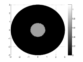
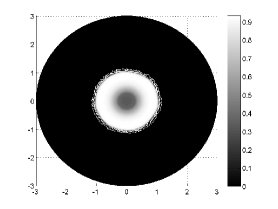
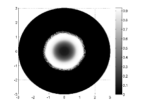
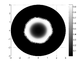
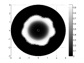
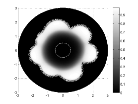
Figure 1: The time dynamics of the density $n$ from initially radially symmetric plateau. The time increases from left to right and from top to bottom.

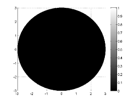
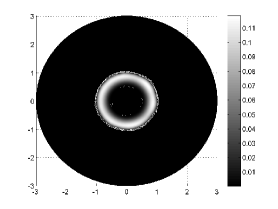
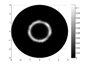
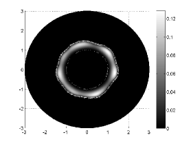
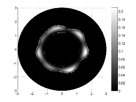
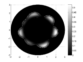
Figure 2: The time evolution of the pressure $P(n)$ from initially radially symmetric plateau. The time increases from left to right and from top to bottom.

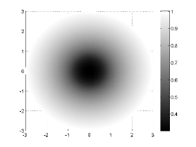
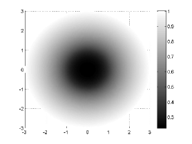
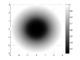
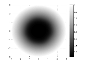
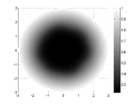
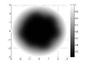
Figure 3: The time evolution of the nutrient distribution $c$ from initially radially symmetric plateau. The time increases from left to right and from top to bottom.

2.2 One dimensional numerical traveling waves

Because we wish to study the invasion process before the instability occurs, we focus on dimension $1$. We present some numerical simulations for the case in vitro given by equation (3) with the following parameters

$$\gamma=50,\qquad\psi(n)=\left\{\begin{array}[]{ll}2,&n\geq 1,\\ 1,&n<1,\end{array}\right.\qquad G(c)=\left\{\begin{array}[]{ll}\ \ 21,&c\geq 0.6,\\ -30,&c<0.6.\end{array}\right.$$ (9)

The computational domain is $[-5,5]$ and we start from an initial plateau

$$n(x)=\left\{\begin{array}[]{ll}0.1,&x\in(-0.5,0.5),\\ \ \ 0,&x\in[-5,-0.5]\cup[0.5,5].\end{array}\right.$$

The boundary condition are as follows:

$$n(-5)=n(5)=0,\qquad c(-5)=c(5)=c_{B}.$$

In order to track the front position, that is the boundary point of the set $\{n>0\}$, and to perform the numerical simulations on the whole domain, we consider different diffusion values inside and outside the tumor region. Therefore, we assume that the diffusion coefficient for $c$ depends on $n$ in such a way that, at time $t$, the nutrient distribution satisfies

$$-\nabla(H(n,t)\nabla c)+\phi(n,t)c=\phi(n,t)(1-H(n,t))c_{B}.$$ (10)

Here $H(n,t)$ gives the front position of $\{n(t)>0\}$ and

$$\phi(n,t)=\left\{\begin{array}[]{ll}\psi(n),&\text{for }\;H(n,t)=1,\\ 1,&\text{for }\;H(n,t)=0.\end{array}\right.$$

More precisely, let $\epsilon$ be some small tolerance (we choose $10^{-5}$ in practice), numerically $H(n,t)$ can be approximated by

$$H(n,t)=\left\{\begin{array}[]{ll}1,&\quad\{n(s)>\epsilon,\mbox{ for some $s\in[0,t]$}\},\\ 0,&\quad\mbox{otherwise}.\end{array}\right.$$

Therefore, the nutrient diffusion coefficient is $1$ inside the tumor while it is worth $0$ outside. Formally, since $\psi(n)\neq 0$ according to (9), the equation (10) is equivalent to write

$$\left\{\begin{array}[]{ll}-\Delta c+\lambda\Psi(n)c=0,&\quad\mbox{for }H(n,T)=1,\\ c=c_{B},&\quad\mbox{for }H(n,T)=0.\end{array}\right.$$

The numerical solutions are displayed in Fig. 4 for six different times. We can see that initially the cell density increases without motion, see subfig. a) and b). After a while, the pressure increases and the front of the tumor begins to move outwards, see subfig. b) and later. As the size of the tumor increases, the cell density in the middle decreases due to the lack of nutrient, see subfig. d) and later. In this one dimensional computation, we finally obtain two plateaus that separate, with tails that enlarge and apparently let a necrotic core appear in the very center (the analytic form show that the cell number density does not really vanish, it is in fact an exponential decay). During all these process, $c$ is constant outside of the tumor as expected.

In order to see the traveling wave solutions, we can use a larger computational domain $[-20,20]$ with the same parameters and initial condition. The results are displayed in Fig. 5. We can observe numerically that the traveling velocities and the sizes of the plateaus increase with $c_{B}$. Besides, the maximum of the pressure for $c_{B}=2$ is almost four times its maximum value for $c_{B}=1$.

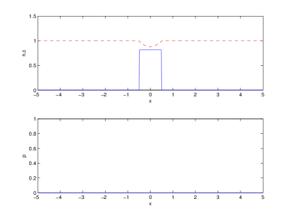
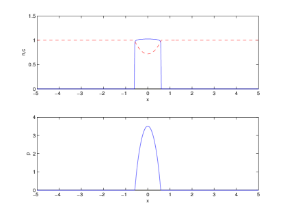
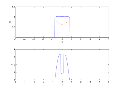
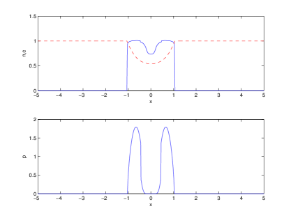
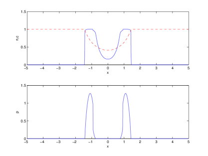
a) b) c) d) e) f)

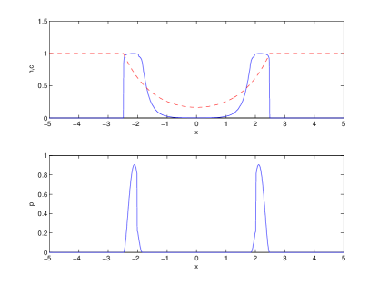
Figure 4: Time dynamics of the system (1). The parameters are chosen as in (9). a), b), c), d), e), f) are for different time and the time increases from a) to f). In each figure, the top subplot depicts the density distribution $n(x)$ (solid line) and nutrient distribution $c(x)$ (dashed line), while the bottom subplot gives the pressure $p(x)$.

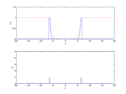
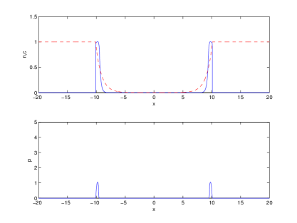
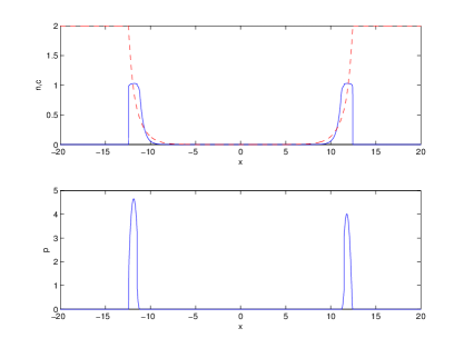
a) b) c) d)

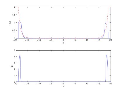
Figure 5: Time dynamics in vitro computed with a larger domain $[-20,20]$. a), b) are for $c_{B}=1$ and c), d) are for $c_{B}=2$. Here a), d) are the results at time $t=1$, b), e) are at $t=1.5$. In each figure, the top subplot depicts the density distribution $n(x)$ (solid line) and nutrient distribution $c(x)$ (dashed line), while the bottom subplot gives the pressure $p(x)$.

In vivo, that is for the equation (4), the traveling waves are displayed in Fig. 6. Here, we use the same values of $\gamma$ and $\psi(n)$ as in (9) but the growth function $G(c)$ is given by

$$G(c)=\left\{\begin{array}[]{ll}\ \ 21,&c\geq 0.3,\\ -30,&c<0.3.\end{array}\right.$$ (11)

With the same initial and boundary conditions as for the in vitro case, the nutrient decreases exponentially from outside of the tumor and wave velocity increases with $c_{B}$. If we keep using the $G(c)$ as in (9), the initial cell density decreases to zero as time goes on.

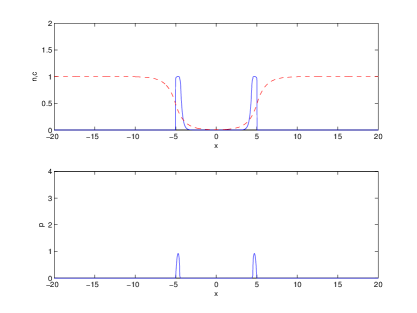
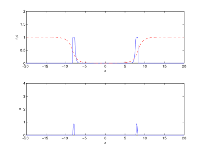
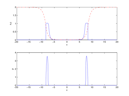
a) b) c) d)

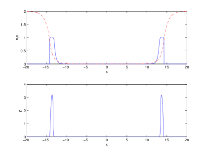
Figure 6: Time dynamics in vivo computed with a larger domain $[-20,20]$. a), b) are for $c_{B}=1$ and c), d) are for $c_{B}=2$. Here a), c) are the results at $T=0.75$ and b), d) are at $T=1$. In each figure, the top subplot depicts the cell distribution $n(x)$ (solid line) and nutrient concentration $c(x)$ (dashed line), while the bottom subplot gives the pressure $p(x)$.

The pressure profiles for both in vitro and in vivo models is displayed in Fig. 7 for $c_{B}=1$ and with the same parameters and initial conditions. Smooth transition of the pressure to the necrotic core can be observed in both cases. Besides the traveling velocity is a bit larger than the one computed analytically in the subsequent part of this paper. This is because additional numerical diffusion is introduced at the front of the pressure. Such phenomena is similar as in simulations of the porous media equation.

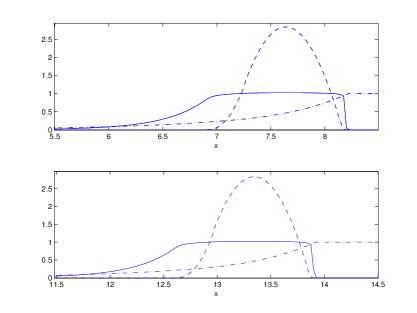
a) b)

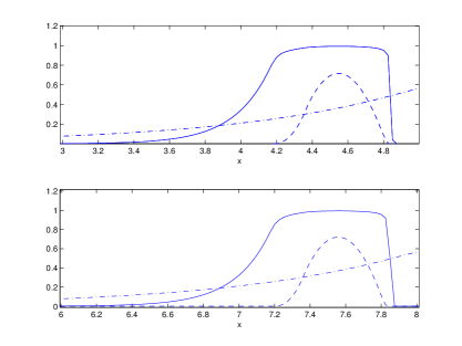
Figure 7: Zoom of the pressure profiles for both in vitro (a) and in vivo (b) models. Results are displayed at $T=0.75$ (top) and $T=1.25$ (bottom) with the same parameters and initial conditions. Each figure depicts cell distribution $n(x)$ (solid line), nutrient concentration $c(x)$ (dash dotted line), and pressure $p(x)$ (dashed line).

3 Traveling waves for a simplified Hele-Shaw model with nutrients

Traveling waves correspond to an established regime and are a convenient way to explain patterns in cancer invasions [3, 27]. Therefore, as observed numerically in the previous section, we can expect existence of traveling waves with a proliferative rim and a necrotic core that invades the domain, at least for large values of $\gamma$ in equation (1) coupled to (4) or (3). It is not our purpose here, to give a general existence proof of such traveling waves for a fixed and finite $\gamma$. Here, we focus on the asymptotic model, which is the following free boundary Hele-Shaw model with nutrients :

$$\left\{\begin{array}[]{ll}\displaystyle\partial_{t}n-{\rm div}(n\nabla p)=nG(c),&\mbox{in $\Omega_{0}(t)$},\qquad\Omega_{0}(t)=\{p(t,x)=0\},\\[2.84526pt] n(x,t)=1&\mbox{in $\Omega(t)$},\qquad\ \ \Omega(t)\;=\{p(t,x)>0\},\\[2.84526pt] -\Delta c+\Psi(n,c)=0,&\displaystyle\lim_{x\to+\infty}c(x)=c_{B},\\[2.84526pt] -\Delta p=G(c),&\mbox{in $\Omega(t)$},\\[2.84526pt] p=0,&\mbox{on $\partial\Omega(t)$}.\end{array}\right.$$ (12)

The growth term $G$ is assumed to satisfy the conditions (8).

Traveling waves are solutions which can be written under the form

$$n(t,x)=n(x\cdot\mathbf{e}-\sigma t),\quad c(t,x)=c(x\cdot\mathbf{e}-\sigma t),\quad p(t,x)=n(x\cdot\mathbf{e}-\sigma t),$$

where $\sigma>0$ is a constant representing the traveling wave velocity. This leads to the following, time independent, system :

$$\left\{\begin{array}[]{ll}-\sigma\mathbf{e}\cdot\nabla n=nG(c),&\mbox{in $\Omega_{0}(t)$},\qquad\Omega_{0}=\{p(x)=0\},\\[2.84526pt] n=1,&\mbox{in $\Omega(t)$},\qquad\ \ \Omega\;=\{p(x)>0\},\\[2.84526pt] -\Delta c+\Psi(n,c)=0,&\displaystyle\lim_{x\to+\infty}c(x)=c_{B},\\[2.84526pt] -\Delta p=G(c),&\mbox{in $\Omega(t)$},\\[2.84526pt] p=0,&\mbox{on $\partial\Omega(t)$}.\end{array}\right.$$ (13)

For the two different models under consideration, in vitro and in vivo, the general equation for $c$ in (13) is defined by (3) and (4) respectively.

3.1 Existence of traveling waves in one dimension in vitro

Focusing on the one dimensional case in vitro, we look for a traveling wave on the real line propagating to the left. Then, we can simplify the system (13) by introducing the parameter $R>0$ such that

$$\Omega=\{p(x)>0\}=[0,R],\qquad\qquad\{n(x)>0\}=(-\infty,R).$$

The above system becomes

$$-\sigma n^{\prime}=nG(c),\quad\mbox{ in }(-\infty,0],$$ (14)

$$n=1\quad\mbox{ on }[0,R],\qquad n=0\ \mbox{ on }(R,+\infty),$$ (15)

$$c^{\prime\prime}=\psi(n)c\ \mbox{ on }(-\infty,R],\qquad c(R)=c_{B},$$ (16)

$$-p^{\prime\prime}=G(c)\quad\mbox{ on }[0,R],\qquad p(0)=p(R)=0,\qquad p\geq 0.$$ (17)

We claim, this can be completed with the following jump relations at $x=0$ and $R$,

$$\sigma=-p^{\prime}(R^{-}),\qquad n(0)=1,\qquad p^{\prime}(0^{+})=0.$$ (18)

Indeed, together with (17), the jump relations at $x=0$ and $R$, for the equation on $n$, give $[\sigma n]+[n\partial_{x}p]=0$. Therefore, denoting $n_{0}=n(0^{-})\in(0,1]$, we arrive at

$$p^{\prime}(0^{+})=-\sigma(1-n_{0}),\qquad p^{\prime}(R^{-})=-\sigma,\qquad n_{0}=n(0^{-})\in(0,1].$$

Since $p$ is constructed as the asymptotic limit of $n^{\gamma}$ when $\gamma\to+\infty$, we restrict our study to nonnegative pressures. However, at the point $0$, we have $p(0)=0$, therefore the derivative should satisfy $p^{\prime}(0^{+})\geq 0$, in order to have $p(x)$ nonnegative when $x>0$ in the neighborhood of $0$. Since $n_{0}\leq 1$, from the above relation, we deduce (18).

Since we wish to build the traveling waves with semi-explicit formulas, we impose additional conditions for the $C^{1}$ functions $G$ and $\psi$ :

$$G^{\prime}\geq 0,\quad\exists\,\bar{c}>0\mbox{ such that }G(c)=-g_{-}<0\mbox{ for }c<\bar{c},\mbox{ and }G(c)>0\mbox{ for }c>\bar{c},$$ (19)

$$\forall\,z\in(0,1),\ \ 0<\psi(z)\leq\psi(1),\quad\psi(0)=0.$$ (20)

This latter assumption is automatically satisfied if $\psi$ is nonincreasing. Also, since $\psi\in C^{1}([0,1])$ and $\psi(0)=0$, it implies in particular that $\int_{0}^{1}\frac{\psi(z)}{z}\,dz<\infty$, a property that is used later on.

With these asumptions, we can state an existence result of a traveling wave solution for the Hele-Shaw system with nutrients

Theorem 3.1

Let us assume that $c_{B}>\bar{c}>0$ and that $G$ and $\psi$ are $C^{1}$ functions satisfying assumptions (19)-(20). Then, there exist $\sigma>0$ and $R>0$ such that the system (14)–(18) admits a solution with $c$ increasing on $(-\infty,R]$, $n$ increasing on $(-\infty,0]$ and $\displaystyle\lim_{x\to-\infty}n(x)=0$.

Proof. The idea of the proof is as follows. We give a value $\sigma>0$ and build a solution $(n_{\sigma},c_{\sigma},p_{\sigma})$ of (14)–(18) just discarding the relation for $\sigma$ in (18). To do so, we need to fix the parameter $R_{\sigma}$. Therefore, we split the line into the necrotic, the proliferative and the healthy regions

$$(0,\infty)=I\cup II\cup III=(-\infty,0)\cup[0,R_{\sigma}]\cup(R_{\sigma},+\infty),$$

and we build the solution successively on each interval.

Then, the value of $\sigma$ is determined by the fixed point problem

$$\sigma=-p_{\sigma}^{\prime}(R_{\sigma}).$$ (21)

Step 1. The piecewise construction of the wave. Fig. 7 can serve as a guide to vizualize the construction which follows. We build the solution departing from the last (healthy) region. Indeed, we have
$\bullet$ On $III=(R,+\infty)$, $n(x)=0$, $p(x)=0$, $c=c_{B}$.
$\bullet$ On $II=[0,R]$, $n(x)=1$. Then, the system reduces to the to solving the equations

$$-c^{\prime\prime}+\psi(1)c=0,\qquad c(R)=c_{B},$$

$$-p^{\prime\prime}=G(c),\qquad p(0)=p^{\prime}(0)=0.$$

Setting $c^{\prime}_{R}=c^{\prime}(R)/\sqrt{\psi(1)}$ which is unknown, we obtain by solving the first equation

$$c(x)=c_{B}\cosh\big{(}\sqrt{\psi(1)}(x-R)\big{)}+c^{\prime}_{R}\sinh\big{(}\sqrt{\psi(1)}(x-R)\big{)}.$$ (22)

For the second equation, we have

$$p(x)=-\int_{0}^{x}\int_{0}^{y}G(c)(z)\,dzdy=-\int_{0}^{x}(x-z)G(c)(z)\,dz.$$ (23)

Moreover, the boundary condition $p(R)=0$, gives

$$\int_{0}^{R}\int_{0}^{y}G\big{(}c_{B}\cosh(\sqrt{\psi(1)}(z-R))+c^{\prime}_{R}\sinh(\sqrt{\psi(1)}(z-R))\big{)}\,dzdy=0.$$

Applying the Fubini theorem, we can rewrite this last equation as

$$\int_{0}^{R}z\,G\left(c_{B}\cosh(\sqrt{\psi(1)}z)-c^{\prime}_{R}\sinh(\sqrt{\psi(1)}z)\right)\,dz=0.$$

Setting $s=z/R$, this nonlinear equation gives a first relation between the two free parameters $R$ and $c^{\prime}_{R}$

$$\int_{0}^{1}s\;G\left(c_{B}\cosh\big{(}\sqrt{\psi(1)}Rs\big{)}-c^{\prime}_{R}\sinh\big{(}\sqrt{\psi(1)}Rs\big{)}\right)\,ds=0.$$ (24)

Moreover, we are looking for a solution $c$ which is positive and nondecreasing. From (22), we have

$$c^{\prime}(x)=c_{B}\sqrt{\psi(1)}\sinh\big{(}\sqrt{\psi(1)}(x-R)\big{)}+c^{\prime}_{R}\sqrt{\psi(1)}\cosh\big{(}\sqrt{\psi(1)}(x-R)\big{)}.$$

Thus, $c$ is positive and nondecreasing on $[0,R]$ iff $c(0)>0$ and $c^{\prime}(0)>0$, that is

$$c_{B}\tanh(\sqrt{\psi(1)}R)\leq c^{\prime}_{R}<\frac{c_{B}}{\tanh(\sqrt{\psi(1)}R)}.$$ (25)

Notice that, with (25) and (24), we have necessarily

$$\bar{c}>c(0)>0\quad\mbox{ and }\quad c^{\prime}(0)\geq 0.$$ (26)

because $G(c)$ has to be negative on a subinterval of $(0,R)$, and monotonicity of $G$ and $c$.

$\bullet$ On $I=(-\infty,0)$, we have $p=0$ and we look for a solution to the system

$$-\sigma n^{\prime}=nG(c),\qquad n(0)=1,$$ (27)

$$c^{\prime\prime}=\psi(n)c,\qquad c(0)=c_{0},\ c^{\prime}(0)=c^{\prime}_{0},$$ (28)

where by continuity for $c$ and $c^{\prime}$ at $0$, from (22) we conclude that

$$\displaystyle c_{0}=c_{B}\cosh(\sqrt{\psi(1)}R)-c^{\prime}_{R}\sinh(\sqrt{\psi(1)}R)<\bar{c},$$ (29)

$$\displaystyle c^{\prime}_{0}=c^{\prime}_{R}\sqrt{\psi(1)}\cosh(\sqrt{\psi(1)}R)-c_{B}\sqrt{\psi(1)}\sinh(\sqrt{\psi(1)}R)>0.$$ (30)

From (19), we deduce that $G(c)=-g_{-}$ on $(-\infty,0]$. Therefore the solution of equation (27) is given by

$$n(x)=e^{\frac{g_{-}}{\sigma}x},\qquad\mbox{for }x<0.$$ (31)

From this, we show in the proof of Lemma 3.2 below, that we can solve the equation on $c$ and deduce the existence of a function $A(\sigma)>0$, for $\sigma>0$, such that $c^{\prime}_{0}=A(\sigma)c_{0}$ and the solution $c$ of (28) is nonnegative and nondecreasing for all $x\in I$.

Step 2. The nonlinear equations for $R_{\sigma}$ and $c^{\prime}_{R}$. Using this function $A(\sigma)>0$ and (29)-(30), we can reduce our construction to the second relation between $R$ and $c^{\prime}_{R}$ (together with (24))

$$c^{\prime}_{R}=c_{B}\frac{A(\sigma)\cosh(\sqrt{\psi(1)}R)+\sqrt{\psi(1)}\sinh(\sqrt{\psi(1)}R)}{A(\sigma)\sinh(\sqrt{\psi(1)}R)+\sqrt{\psi(1)}\cosh(\sqrt{\psi(1)}R)}.$$ (32)

Notice that, from this expression, a simple but tedious calculation shows that (25) is satisfied.

Finally, for a given $\sigma>0$, we have constructed a possible solution on $(-\infty,R_{\sigma}]$ such that $c$ is nondecreasing and $\lim_{x\to-\infty}c(x)=c_{-}\geq 0$. To conclude the construction, we need to prove that there exists $R_{\sigma}>0$, $c^{\prime}_{R}>0$ such that (24) and (32) are satisfied.

We define, using (32),

$$\begin{array}[]{ll}\displaystyle\gamma_{\sigma}(R,s)&:=\displaystyle c_{B}\cosh(\sqrt{\psi(1)}Rs)-c^{\prime}_{R}\sinh(\sqrt{\psi(1)}Rs)\\[8.53581pt] &\displaystyle=c_{B}\frac{A(\sigma)\sinh(\sqrt{\psi(1)}R(1-s))+\sqrt{\psi(1)}\cosh(\sqrt{\psi(1)}R(1-s))}{A(\sigma)\sinh(\sqrt{\psi(1)}R)+\sqrt{\psi(1)}\cosh(\sqrt{\psi(1)}R)}.\end{array}$$ (33)

Then, the equation (24) is also written,

$$\int_{0}^{1}sG(\gamma_{\sigma}(R_{\sigma},s))ds=0.$$

We are going to show that there is a unique solution $R_{\sigma}>0$, continuous with respect to $\sigma$. Firstly, from a straightforward computation, (33) shows that for all $s\in(0,1)$

$$\begin{array}[]{ll}\displaystyle\frac{d}{dR}\gamma_{\sigma}(R,s)<&\displaystyle\frac{c_{B}\sqrt{\psi(1)}\sinh(\sqrt{\psi(1)}Rs)\big{(}A(\sigma)^{2}-\psi(1)\big{)}}{\Big{(}A(\sigma)\sinh(\sqrt{\psi(1)}R)+\sqrt{\psi(1)}\cosh(\sqrt{\psi(1)}R)\Big{)}^{2}}.\end{array}$$

With the estimate of Lemma 3.2, we deduce that $R\mapsto\gamma_{\sigma}(R,s)$ is a decreasing function for all $s\in(0,1)$. By monotonicity of $G$ in (19) we deduce that $R\mapsto\int_{0}^{1}sG(\gamma_{\sigma}(R,s))\,ds$ is a decreasing function. When $R=0$, we have $\gamma_{\sigma}(0,s)=c_{B}$, then $\int_{0}^{1}sG(\gamma_{\sigma}(0,s))\,ds=G(c_{B})/2>0$. When $R\to+\infty$, we have $\gamma_{\sigma}(R,s)\sim e^{-\sqrt{\psi(1)}Rs}\to 0$ for $s>0$; then $\int_{0}^{1}sG(\gamma_{\sigma}(R,s))\,ds\to G(0)/2<0$. By continuity and monotonicity, we conclude on the existence of a unique $R_{\sigma}>0$ such that (24) is satisfied. Secondly, by continuity of $\sigma\mapsto A(\sigma)$, we deduce that $\sigma\mapsto R_{\sigma}$ is continuous.

Step 3. The nonlinear equation for $\sigma$. We are reduced to proving the existence of a solution for the fixed point problem (21). Thanks to the expression of the pressure, (23), we can rewrite the equation as

$$\sigma=R_{\sigma}\int_{0}^{1}G\left(c_{B}\cosh(\sqrt{\psi(1)}R_{\sigma}s)-c^{\prime}_{R}\sinh(\sqrt{\psi(1)}R_{\sigma}s)\right)\,ds,$$

where $c^{\prime}_{R}$ is defined by (32). With the expression of $\gamma_{\sigma}$ given in (33), the latter equation rewrites

$$\sigma=R_{\sigma}\int_{0}^{1}G\big{(}\gamma_{\sigma}(R_{\sigma},s)\big{)}\,ds.$$ (34)

We first notice that from Lemma 3.2, we have $A(\sigma)\to 0$ when $\sigma\to 0$. We deduce that $R_{\sigma}\to R_{0}>0$ which is a solution to

$$\int_{0}^{1}sG(\gamma_{\sigma}(R_{0},s))\,ds=\int_{0}^{1}sG\Big{(}c_{B}\frac{\cosh(\sqrt{\psi(1)}R_{0}(1-s))}{\cosh(\sqrt{\psi(1)}R_{0})}\Big{)}\,ds=0.$$

Since $s\mapsto\gamma_{\sigma}(R_{0},s)$ is nonincreasing, there exists $s_{0}\in(0,1)$ such that $G(\gamma_{\sigma}(R_{0},s))\geq 0$ for all $s<s_{0}$ and $G(\gamma_{\sigma}(R_{0},s))<0$ for all $s>s_{0}$. We deduce that

$$0=\int_{0}^{1}sG(\gamma_{\sigma}(R_{0},s))\,ds<s_{0}\int_{0}^{1}G(\gamma_{\sigma}(R_{0},s))\,ds.$$

Then the limit when $\sigma\to 0$ of the right hand side of (34) is positive. On the other hand, from the lower bound of $c^{\prime}_{R}$ in (25), we have that $\displaystyle\gamma_{\sigma}(R,s)\leq\frac{c_{B}}{\cosh(\sqrt{\psi(1)}Rs)}$. It is straightforward to verify that there is a unique $R_{b}>0$ such that

$$\int_{0}^{1}sG\Big{(}\frac{c_{B}}{\cosh(\sqrt{\psi(1)}R_{b}s)}\Big{)}\,ds=0.$$

We deduce that for all $R\geq R_{b}$ we have, by monotonicity of $G$,

$$\int_{0}^{1}sG(\gamma_{\sigma}(R,s))\,ds\leq\int_{0}^{1}sG\Big{(}\frac{c_{B}}{\cosh(\sqrt{\psi(1)}Rs)}\Big{)}\,ds\leq\int_{0}^{1}sG\Big{(}\frac{c_{B}}{\cosh(\sqrt{\psi(1)}R_{b}s)}\Big{)}\,ds=0.$$

Since $\int_{0}^{1}sG(\gamma_{\sigma}(R_{\sigma},s))\,ds=0$, we conclude that $0<R_{\sigma}\leq R_{b}$. Thus the right hand side of (34) is bounded. By continuity, we conclude that equation (34) admits a solution $\sigma>0$.       

3.2 A technical Lemma

In the proof of Theorem 3.1, we have used an argument which is stated in the

Lemma 3.2

Let $\sigma>0$ and $g_{-}>0$ be given and assume that $\psi$ satisfies (20). We consider the Cauchy problem

$$-c^{\prime\prime}+\psi\big{(}e^{g_{-}x/\sigma}\big{)}c=0\;\text{for }x<0,\qquad c(0)=c_{0},\quad c^{\prime}(0)=c^{\prime}_{.}$$ (35)

Then, there exists a continuous mapping $\sigma\mapsto A(\sigma)\in(0,\sqrt{\psi(1)}\,]$ such that the solution of the Cauchy problem (35) is defined, nonnegative and nondecreasing, if and only if $c^{\prime}_{0}=A(\sigma)c_{0}$. Moreover, the estimate holds : $A(\sigma)\leq\frac{\sigma}{g_{-}}\int_{0}^{1}\frac{\psi(\nu)}{\nu}\,d\nu$ and $A(\cdot)$ can be extended by continuity to $A(0)=0$.

Proof. We first reduce equation (35) to the following ODE system,

$$c^{\prime}=u,\qquad c(0)=c_{0},$$ (36)

$$u^{\prime}=\psi\big{(}e^{g_{-}x/\sigma}\big{)}c,\qquad u(0)=c^{\prime}_{0}.$$ (37)

Since we are looking for a nondecreasing $c$, we have $u\geq 0$. This system can be further simplified by setting $y=-e^{g_{-}x/\sigma}$. We define $\widetilde{u}(y)=u(x)/c_{0}$ and $\widetilde{c}(y)=c(x)/c_{0}$. Then system (36)–(37), reduces to a Cauchy problem on $[-1,0]$ :

$$\left\{\begin{array}[]{ll}\displaystyle\frac{d\widetilde{c}}{dy}=\frac{\sigma}{g_{-}y}\,\widetilde{u},\qquad\frac{d\widetilde{u}}{dy}=\frac{\sigma\psi(-y)}{y\,g_{-}}\,\widetilde{c},\\[8.53581pt] \displaystyle\widetilde{c}(-1)=1,\qquad\quad\widetilde{u}(-1)=c^{\prime}_{0}/c_{0}.\end{array}\right.$$ (38)

There exists a unique solution to this Cauchy problem and $\widetilde{u}$ is nonincreasing and $\widetilde{c}$ is nonincreasing until $\widetilde{u}$ vanishes. Thus there are two kinds of solutions :

• either there exists $y_{0}\in(-1,0)$ such that $\widetilde{u}(y_{0})=0$, this solution is called Type I,

• or $\widetilde{u}>0$ on $(-1,0)$, this solution is called Type II.

Obviously, we are looking for a solution in the limiting case, where $y_{0}=0$ and $\widetilde{u}(y)>0$ for all $y\in[-1,0)$.

We first notice that if $c^{\prime}_{0}=0$, then clearly the solution is of Type I. On the contrary, if we assume that all the solutions are of Type I, then on $(-1,y_{0})$, we have $0\leq\widetilde{c}\leq 1$. It implies from (38) that for $y\in(-1,y_{0})$, ($y_{0}<0$)

$$\frac{d\widetilde{u}}{dy}=\frac{\sigma\psi(-y)\widetilde{c}}{g_{-}y}\geq\frac{\sigma\psi(-y)}{g_{-}y}.$$

Integrating on $[-1,y_{0}]$, we deduce that

$$\widetilde{u}(y_{0})\geq\frac{c^{\prime}_{0}}{c_{0}}+\frac{\sigma}{g_{-}}\int_{-1}^{y_{0}}\frac{\psi(-\nu)}{\nu}\,d\nu.$$

The integral in the right hand side is finite thanks to assumption (20). We deduce that if $c^{\prime}_{0}$ is large enough such that

$$\frac{c^{\prime}_{0}}{c_{0}}+\frac{\sigma}{g_{-}}\int_{-1}^{y_{0}}\frac{\psi(-\nu)}{\nu}\,d\nu>0,$$ (39)

then $\widetilde{u}(y_{0})>0$ which contradicts the fact that $\tilde{u}(y_{0})=0$.

In summary, for $c^{\prime}_{0}=0$ the solution is of Type I, for $c^{\prime}_{0}$ large enough the solution is of Type II. By continuity wich respect to the initial data, there exists $c^{\prime}_{0}$ such that the Cauchy problem (38) admits a solution such that $y_{0}=0$ and $\widetilde{u}(y)>0$ for all $y\in[-1,0)$.

From now on, we denote $A(\sigma)=\widetilde{u}(-1)=\frac{c^{\prime}_{0}}{c_{0}}$ to emphasize the dependency on $\sigma$. Besides, from (39), when $c_{0}^{\prime}/c_{0}>-\frac{\sigma}{g_{-}}\int_{-1}^{0}\frac{\psi(-\nu)}{\nu}\,d\nu$, the solution is of type II. Thus we have obviously

$$A(\sigma)<-\frac{\sigma}{g_{-}}\int_{-1}^{0}\frac{\psi(-\nu)}{\nu}\,d\nu=\frac{\sigma}{g_{-}}\int_{0}^{1}\frac{\psi(\nu)}{\nu}\,d\nu\quad\forall\sigma>0.$$

Then from the continuity of the Cauchy problem (38) with respect to the parameter $\sigma$ and with respect to the initial data, we deduce that $A(\cdot)$ is continuous.

Moreover, we clearly have from (38)

$$\widetilde{u}\frac{d\widetilde{u}}{dy}=\widetilde{c}\frac{d\widetilde{c}}{dy}\psi(-y).$$

We have established the existence of $\widetilde{c}$ which is nonnegative and nonincreasing on $(-1,0)$. Therefore, since $\psi(-y)\leq\psi(1)$ from assumption (20), we deduce

$$\frac{d\widetilde{u}^{2}}{dy}\geq\frac{d\widetilde{c}^{2}}{dy}\psi(1).$$

Integrating on $(-1,0)$ we obtain

$$\widetilde{u}^{2}(0)-\widetilde{u}^{2}(-1)\geq\psi(1)(\widetilde{c}^{2}(0)-\widetilde{c}^{2}(-1))\geq-\psi(1).$$

By definition $A(\sigma)=\widetilde{u}(-1)$ and with the boundary conditions in (38), we conclude that the estimate $A(\sigma)\leq\sqrt{\psi(1)}$ holds.       

3.3 Analytical example

The Theorem 3.1 can be illustrated thanks to an explicit traveling wave, in the particular case when

$$\psi(n)=\left\{\begin{array}[]{ll}\lambda,&n=1,\\ \lambda n_{c},&n<1,\\ 0,&n=0.\end{array}\right.\qquad G(c)=\left\{\begin{array}[]{ll}\ \ g_{+},&\quad c>\bar{c},\\ -g_{-},&\quad c<\bar{c}.\end{array}\right.$$ (40)

with $\lambda$, $n_{c}$, $g_{+}$, $g_{-}$ some positive constants and $n_{c}<1$. We can not apply directly Theorem 3.1 since the functions $G$ and $\psi$ are not $C^{1}$. However, with this simple choice, we are able to manage explicit calculations and therefore state the following existence result :

Theorem 3.3

Let $c_{B}>\bar{c}>0$ and let $\psi(n)$, $G(c)$ be chosen as in (40). There exists an unique monotone traveling wave for the Hele-Shaw model with nutrient i.e. an unique positive $\sigma$ and $R>0$ such that the system (14)–(18) admits a nonnegative solution with $c^{\prime}\geq 0$. Moreover we have

$$\sigma=R\;\big{(}\sqrt{(g_{+}+g_{-})g_{-}}-g_{-}\big{)},$$ (41)

where the value $R$ is obtained by solving (48) below. The velocity $\sigma$ increases with respect to $c_{B}$ and decreases with respect to $\bar{c}$.

Proof. We use the same strategy as in the previous Section. Let $\sigma>0$ be given. We divide the whole real line into $I\cup II\cup III=(-\infty,0]\cup(0,R)\cup[R,+\infty)$.

$\bullet$ In $III=[R,+\infty)$, $n(x)=0$, $p(x)=0$, $c(x)=c_{B}$.
$\bullet$ In $II=(0,R)$, $n(x)=1$ and $c(x)$ satisfies

$$-\partial_{xx}c+\lambda c=0,\qquad c(R)=c_{B},\quad c^{\prime}(R)=c^{\prime}_{R}.$$

As above, we have then that

$$c(x)=c_{B}\cosh(\sqrt{\lambda}(x-R))+c^{\prime}_{R}\sinh(\sqrt{\lambda}(x-R)).$$

This function is positive and nondecreasing provided (see (25))

$$c_{B}\tanh(\sqrt{\lambda}R)\leq c^{\prime}_{R}<\frac{c_{B}}{\tanh(\sqrt{\lambda}R)}.$$ (42)

Consider the equation for $p$ : $-\partial_{xx}p=G(c)$. On the one hand, we have $p(0)=0$ and $p^{\prime}(0)=0$ from (18). If we want $p$ to take nonnegative values, it has to be convex at $0$. Therefore from (17) we deduce $G(c(0))=-g_{-}<0$, i.e. $c(0)<\bar{c}$ from (40). Then we solve $-\partial_{xx}p=-g_{-}$ with boundary conditions $p(0)=0$, $p^{\prime}(0)=0$, which yields

$$p(x)=\frac{g_{-}}{2}x^{2},\qquad x\in(0,x_{1}),\quad\mbox{where}\quad c(x_{1})=\bar{c}.$$

Since $c(x)$ is nondecreasing provided (42) is satisfied, $x_{1}>0$ and from $p(R)=0$, we have $R>x_{1}$. We can determine $x_{1}$ by $c(x_{1})=\bar{c}$ such that

$$c_{B}\cosh(\sqrt{\lambda}(x_{1}-R))+c^{\prime}_{R}\sinh(\sqrt{\lambda}(x_{1}-R))=\bar{c}.$$ (43)

On the interval $x\in(x_{1},R)$, $G(c(x))=g_{+}$ so that $-\partial_{xx}p=g_{+}$. Solving this equation with continuity of $p$ and $p^{\prime}$ at $x_{1}$, we obtain

$$p(x)=-\frac{g_{+}}{2}(x-x_{1})^{2}+g_{-}x_{1}(x-x_{1})+\frac{x_{1}^{2}}{2}g_{-},\qquad x\in(x_{1},R).$$

Then, from $p(R)=0$, we have

$$-\frac{g_{+}}{2}(R-x_{1})^{2}+g_{-}x_{1}(R-x_{1})+\frac{x_{1}^{2}}{2}g_{-}=0.$$ (44)

Additionally, we recall the jump condition $\sigma=-p^{\prime}(R)$ which gives

$$\sigma=g_{+}R-(g_{+}+g_{-})x_{1}.$$ (45)

$\bullet$ In the interval $I=(-\infty,0)$, $p(x)=0$. Since $c(x)\leq c(0)<\bar{c}$, we have $-\sigma n^{\prime}=-g_{-}n$. Together with the boundary conditions $n(0)=1$ (see (18)), we find

$$n(x)=e^{\frac{g_{-}}{\sigma}x}.$$

Then $c(x)$ satisfies $-\partial_{xx}c+\lambda n_{c}c=0$, together with the continuity of $c$ and $c^{\prime}$ at $0$, we get

$$c(x)=\frac{1}{2}\Big{(}c_{0}+\frac{c^{\prime}_{0}}{\xi}\Big{)}e^{\xi x}+\frac{1}{2}\Big{(}c_{0}-\frac{c^{\prime}_{0}}{\xi}\Big{)}e^{-\xi x},\qquad\mbox{ with }\xi=\sqrt{\lambda n_{c}},$$

where the expressions of $c_{0}$ and $c^{\prime}_{0}$ are given in (29)–(30). In order to have $c$ bounded on $(-\infty,0)$, the coefficient in front of $e^{-\xi x}$ has to be zero :

$$c_{0}-\frac{c^{\prime}_{0}}{\xi}=0.$$ (46)

Then we have $\displaystyle c(x)=c_{0}e^{\xi x}$. We observe that $c(x)\geq 0$ for $x\in(-\infty,0)$ provided (42) is satisfied.

With this construction, we have to solve the three equations (43), (44) and (46), for the three unknowns : $c^{\prime}_{R}$, $x_{1}$, $R$. In fact, we notice that all these equations are independent of $\sigma$; more precisely, compared to the proof of Theorem 3.1, we have $A(\sigma)=\xi$ from (46). Then (45) will give the velocity $\sigma$. First, we recover from (46),

$$c^{\prime}_{R}=c_{B}\frac{\xi\cosh(\sqrt{\lambda}R)+\sqrt{\lambda}\sinh(\sqrt{\lambda}R)}{\xi\sinh(\sqrt{\lambda}R)+\sqrt{\lambda}\cosh(\sqrt{\lambda}R)}.$$ (47)

This identity is equivalent to (32) with $A(\sigma)=\xi$. We notice that this expression implies that (42) is satisfied. Then we solve equation (44) and obtain

$$x_{1}=R\Big{(}1-\sqrt{\frac{g_{-}}{g_{+}+g_{-}}}\Big{)}.$$

We set

$$\alpha:=\sqrt{\frac{g_{-}}{g_{+}+g_{-}}}\in(0,1).$$

Finally, substituting $x_{1}=(1-\alpha)R$ and (47) into (43), we obtain the following nonlinear equation for $R>0$ :

$${\cal F}(R):=\frac{\bar{c}}{c_{B}}\Big{(}\cosh(\sqrt{\lambda}R)+\sqrt{n_{c}}\sinh(\sqrt{\lambda}R)\Big{)}-\sqrt{n_{c}}\sinh(\sqrt{\lambda}(1-\alpha)R)-\cosh(\sqrt{\lambda}(1-\alpha)R)=0.$$ (48)

The function ${\cal F}$ is $C^{\infty}(\mathbb{R}_{+})$ and we prove below that there exists an unique positive root for this function. Then we obtain the expression (41) for the velocity from equation (45).

Let us state the existence of an unique positive root for ${\cal F}$. We have ${\cal F}(0)=(\frac{\bar{c}}{c_{B}}-1)<0$, and ${\cal F}(R)\to+\infty$ when $R\to+\infty$. Then there exists a positive root for ${\cal F}$. To prove the uniqueness of this root, let us first choose $k\in\mathbb{N}^{*}$ such that $(1-\alpha)^{k}\leq\frac{\bar{c}}{c_{B}}$ and $(1-\alpha)^{k-1}>\frac{\bar{c}}{c_{B}}$. For every $i\in\mathbb{N}$, we compute the $i$th derivative of ${\cal F}$ from (48) :

$$\begin{array}[]{ll}\displaystyle{\cal F}^{(2i)}(R)=&\displaystyle\sqrt{\lambda}^{{2}i}\Big{(}\frac{\bar{c}}{c_{B}}\big{(}\cosh(\sqrt{\lambda}R)+\sqrt{n_{c}}\sinh(\sqrt{\lambda}R)\big{)}\\[5.69054pt] &\displaystyle\quad-(1-\alpha)^{2i}\big{(}\sqrt{n_{c}}\sinh(\sqrt{\lambda}(1-\alpha)R)+\cosh(\sqrt{\lambda}(1-\alpha)R)\big{)}\Big{)}.\\ \displaystyle{\cal F}^{(2i+1)}(R)=&\displaystyle\sqrt{\lambda}^{2i+1}\Big{(}\frac{\bar{c}}{c_{B}}\big{(}\sinh(\sqrt{\lambda}R)+\sqrt{n_{c}}\cosh(\sqrt{\lambda}R)\big{)}\\[5.69054pt] &\displaystyle\quad-(1-\alpha)^{2i+1}\big{(}\sqrt{n_{c}}\cosh(\sqrt{\lambda}(1-\alpha)R)+\sinh(\sqrt{\lambda}(1-\alpha)R)\big{)}\Big{)}.\end{array}$$

For all $i\geq 0$, we have ${\cal F}^{(i)}(R)\to+\infty$ as $R\to+\infty$. Thanks to our choice for $k$, we have ${\cal F}^{(k)}(R)>0$ for all $R>0$ and ${\cal F}^{(k-1)}(0)<0$. Thus ${\cal F}^{(k-1)}$ is increasing and admits a unique root denoted $r_{k-1}$. Therefore, if $k=1$ we have proved the result. Else, we have then ${\cal F}^{(k-2)}$ is a nonincreasing function on $(0,r_{k-1})$ and an increasing function on $(r_{k-1},+\infty)$. We have from our choice of $k$ that ${\cal F}^{(k-2)}(0)<0$, then ${\cal F}^{(k-2)}(r_{k-1})<0$. Since ${\cal F}^{(k-2)}(R)\to+\infty$ as $R\to+\infty$, we conclude that ${\cal F}^{(k-2)}$ admits an unique positive root $r_{k-2}$. Therefore, if $k=2$ we have proved the result, else we continue and by induction we prove by the same token that ${\cal F}$ is nonincreasing on $(0,r_{1})$, increasing on $(r_{1},+\infty)$ with ${\cal F}(r_{1})\leq{\cal F}(0)<0$ and $\lim_{R\to+\infty}{\cal F}(R)=+\infty$. Thus ${\cal F}$ admits an unique positive root.

Moreover, from the expression of ${\cal F}$ in (48), we deduce clearly that $\displaystyle\frac{\partial{\cal F}}{\partial c_{B}}<0$ and $\displaystyle\frac{\partial{\cal F}}{\partial\bar{c}}>0$. Thus we deduce that $R$ increases with respect to $c_{B}$ and decreases with respect to $\bar{c}$. From (41), we conclude the proof.       

The situation here is simpler than in Theorem 3.1. Indeed, we can compute $R$ as the root of an explicit function (48) which only depends on the parameters. Then we have an analytic expression both of the shape of the wave and of the velocity.

Some consequences of Theorem 3.3 are compatible with the biological intuition. For example, the traveling velocity increases with the nutrient density outside of the tumor, and decreases with $\bar{c}$ which is the critical nutrient density for the growth of tumor cells.

4 Traveling waves for the in vivo case in one dimension

The only difference between in vivo and in vitro models, is the equation for the nutrient availability. The one dimensional in vivo model reads :

$$\left\{\begin{array}[]{ll}-\sigma\partial_{x}n=nG(c),&\mbox{in }\mathbb{R}\setminus(0,R),\\[2.84526pt] n=1&\mbox{in }(0,R),\\[2.84526pt] -\partial_{xx}c+\psi(n)c={1{\rm I}}_{\{n=0\}}(c_{B}-c),&x\in\mathbb{R},\\[2.84526pt] \displaystyle\lim_{x\to+\infty}c(x)=c_{B},\\[2.84526pt] -\partial_{xx}p=G(c),&\mbox{in }(0,R),\\[2.84526pt] p(0)=p(R)=0.\end{array}\right.$$ (49)

This system is still complemented with the jump condition (18). Then, we can adapt the result in Section 3 and prove the following theorem.

Theorem 4.1

Let $\displaystyle 0<\bar{c}<\frac{c_{B}}{2}$ be given. Assume that $G$ and $\psi$ are $C^{1}$ function satisfying (19)–(20). Then, there exist $\sigma>0$ and $R>0$ such that the system (49) together with the jump condition (18) admits a solution with $c$ increasing on $\mathbb{R}$; moreover $n$ is increasing on $(-\infty,0]$ and $\lim_{x\to-\infty}n(x)=0$.

Proof. The idea of the proof is the same as the proof of Theorem 3.1. We will only give the main changes and do not provide all the details of the calculations.
Step 1. The piecewise construction of the wave. Let us assume that $\sigma>0$ is given. We construct the solution for $R>0$ following the proof of Theorem 3.1. We just explain below the main changes :

• On $III=(R,+\infty)$, the only change is for $c$ : $c(x)=c_{B}-c^{\prime}_{R}e^{\sqrt{\psi(1)}(R-x)}$.

• On $II=[0,R]$, the equations are the same but the boundary conditions for $c$ at $x=R$ changes. Then we get

  $$c(x)=c_{B}\cosh\big{(}\sqrt{\psi(1)}(x-R)\big{)}-c^{\prime}_{R}e^{-\sqrt{\psi(1)}(x-R)},$$ (50)

  which is nondecreasing and positive provided

  $$\frac{c_{B}}{2}\Big{(}1-e^{-2\sqrt{\psi(1)}R}\Big{)}\leq c^{\prime}_{R}<\frac{c_{B}}{2}\Big{(}1+e^{-2\sqrt{\psi(1)}R}\Big{)}.$$ (51)

  The pressure is given by expression (23); we deduce, from the boundary condition $p(R)=0$, a similar condition for $R$ as in (24)

  $$\int_{0}^{1}sG\Big{(}c_{B}\cosh\big{(}\sqrt{\psi(1)}Rs\big{)}-c^{\prime}_{R}e^{\sqrt{\psi(1)}Rs}\Big{)}\,ds=0.$$ (52)

• On $I=(-\infty,R)$, applying Lemma 3.2, in order to have the existence of a solution of the system on $I=(-\infty,0)$ such that $c$ is nonnegative and nondecreasing, we introduce a nonnegative function $A(\sigma)$ such that $c^{\prime}(0)=A(\sigma)c(0)$. Injecting the expressions of $c(0)$ and $c^{\prime}(0)$ from (50) into this identity, we deduce

  $$c^{\prime}_{R}=\frac{c_{B}}{2}\Big{(}1+\frac{A(\sigma)-\sqrt{\psi(1)}}{A(\sigma)+\sqrt{\psi(1)}}e^{-2\sqrt{\psi(1)}R}\Big{)}.$$ (53)

  We deduce then that (51) is satisfied.

Step 2. The nonlinear equation for $R$ and $c^{\prime}_{R}$. To conclude the construction, it suffices to show that the nonlinear equation (52) admits a solution $R_{\sigma}$. Let us first introduce the notation

$$\gamma_{\sigma}(R,s):=c_{B}\cosh(\sqrt{\psi(1)}Rs)-c^{\prime}_{R}e^{\sqrt{\psi(1)}Rs},\qquad\mbox{for }s\in(0,1).$$

With (53), we deduce that

$$\gamma_{\sigma}(R,s)=\frac{c_{B}}{2}\Big{(}e^{-\sqrt{\psi(1)}Rs}+\frac{\sqrt{\psi(1)}-A(\sigma)}{A(\sigma)+\sqrt{\psi(1)}}e^{\sqrt{\psi(1)}R(s-2)}\Big{)}.$$ (54)

Then (52) rewrites $\int_{0}^{1}sG(\gamma_{\sigma}(R,s))ds=0$. From the estimate $A(\sigma)\leq\sqrt{\psi(1)}$ in Lemma 3.2, we deduce straightforwardly that $R\mapsto\gamma_{\sigma}(R,s)$ is decreasing for $s\in(0,1)$. With (54) we have $\displaystyle\gamma_{\sigma}(0,s)=c_{B}\frac{\sqrt{\psi(1)}}{A(\sigma)+\sqrt{\psi(1)}}$ and $\displaystyle\lim_{R\to+\infty}\gamma_{\sigma}(R,s)=0$. Since $G(0)<0$, we deduce that $\int_{0}^{1}sG(\gamma_{\sigma}(R,s))ds$ takes negative value for large $R$. From Lemma 3.2, we have $A(\sigma)\leq\sqrt{\psi(1)}$. Then, $\gamma_{\sigma}(0,s)\geq c_{B}/2$. By assumption $\bar{c}<c_{B}/2$, we deduce then from (19) that $\int_{0}^{1}sG(\gamma_{\sigma}(0))ds>0$. By continuity and monotonicity, there exists a unique $R_{\sigma}>0$ such that (52) is satisfied. Moreover, as above, the mapping $\sigma\mapsto R_{\sigma}$ is continuous.

Then for all $\sigma>0$, we have constructed $R_{\sigma}$ and a solution $(n_{\sigma},c_{\sigma},p_{\sigma})$ to the system (49).

Step 3. The nonlinear equation for $\sigma$. It suffices now to prove that there exists $\sigma>0$ such that $\sigma=-p^{\prime}_{\sigma}(R_{\sigma})$, which can be rewritten :

$$\sigma=R_{\sigma}\int_{0}^{1}G\big{(}c_{B}\cosh(\sqrt{\psi(1)}R_{\sigma}s)-c^{\prime}_{R}e^{\sqrt{\psi(1)}R_{\sigma}s}\big{)}\,ds.$$ (55)

Moreover, since we have for all $R>0$,

$$\gamma_{\sigma}(R)\leq\frac{c_{B}}{2}e^{-\sqrt{\psi(1)}Rs}\Big{(}1+e^{-\sqrt{\psi(1)}Rs}\Big{)},$$

we deduce that $R_{\sigma}\leq R_{b}$, where $R_{b}$ is the unique solution of the equation

$$\int_{0}^{1}sG\Big{(}\frac{c_{B}}{2}e^{-\sqrt{\psi(1)}Rs}\big{(}1+e^{-\sqrt{\psi(1)}Rs}\big{)}\Big{)}\,ds=0.$$

By the same token as in the proof of Theorem 3.1, we have that the right hand side of (55) is bounded and admits a positive and finite limit when $\sigma\to 0$. Therefore, by continuity, there exists $\sigma>0$ such that (55) is satisfied.       

Remark 4.2

Notice that the condition $\bar{c}<c_{B}/2$ can be understood from the requirement that $c(0)<\bar{c}<c(R)$. From the expression of $\gamma_{\sigma}(R,s)$ in (54),

$$c(0)=c_{B}e^{-\sqrt{\psi(1)}R}\frac{\sqrt{\psi(1)}}{A(\sigma)+\sqrt{\psi}},\qquad c(R)=\frac{c_{B}}{2}\left(1-\frac{A(\sigma)-\sqrt{\psi(1)}}{A(\sigma)+\sqrt{\psi(1)}}e^{-2\sqrt{\psi(1)}R}\right).$$

For fixed $A(\sigma)$, both $c(0)$ and $c(R)$ decrease with $R$. Moreover, when $R\to+\infty$, $c(0)\to 0$ and $c(R)\to c_{B}/2$, while when $R\to 0$, $c(0)=c(R)=c_{B}\frac{\sqrt{\psi(1)}}{A(\sigma)+\sqrt{\psi(1)}}$. Therefore, when $\bar{c}<c_{B}/2$, $\bar{c}<c(R)$ holds for any $R$. Furthermore, $R$ big enough gives $c(0)<\bar{c}$.

This condition confirms our numerical observations in Section 2. In fact, for the in vivo model, we have noticed that traveling waves do not exist when we use the expression in (9) for the growth function for which the condition $\bar{c}<c_{B}/2$ is violated. But if we choose (11) instead, numerical simulations exhibits traveling waves (see Fig. 6).

Analytical example.

Following the previous section, we consider the case where the nutrient consumption $\psi$ and the growth term $G$ are given by (40). Then, we have the

Proposition 4.3

Let $\displaystyle 0<\bar{c}<\frac{c_{B}}{2}$ and assume that (40) holds true with $n_{c}<1$. Then there exists a unique traveling wave. Moreover, its velocity is given by

$$\sigma=R\big{(}\sqrt{(g_{+}+g_{-})g_{-}}-g_{-}\big{)},$$

where $R$ is the solution to (56). Moreover, $\sigma$ is nondecreasing with respect to $c_{B}$ and nonincreasing with respect to $\bar{c}$.

Proof. As in Theorem 4.1, in the region $[0,R]$, the nutrient concentration $c(x)$ can be given by (50) with $\psi(1)=\lambda$. As has been stated in the proof of Theorem 3.3 that when $\psi(n)$, $G(n)$ are as in (40), we have $A(\sigma)=\sqrt{\lambda n_{c}}$. Thus identity (53) becomes

$$c^{\prime}_{R}=\frac{c_{B}}{2}\Big{(}1-\frac{1-\sqrt{n_{c}}}{1+\sqrt{n_{c}}}e^{-2\sqrt{\lambda}R}\Big{)}.$$

From the proof of Theorem 3.3, let $c(x_{1})=\bar{c}$, the equation for the pressure indicates that $x_{1}=(1-\sqrt{\frac{g_{-}}{g_{+}+g_{-}}})R=(1-\alpha)R$ with $\alpha=\sqrt{\frac{g_{-}}{g_{+}+g_{-}}}$. Then, from (50), the nonlinear equation for the unknonw $R$ is :

$$c_{B}\cosh(\sqrt{\lambda}\alpha R)-\frac{c_{B}}{2}\Big{(}1-\frac{1-\sqrt{n_{c}}}{1+\sqrt{n_{c}}}e^{-2\sqrt{\lambda}R}\Big{)}e^{\alpha\sqrt{\lambda}R}=\bar{c},\qquad\alpha=\sqrt{\frac{g_{-}}{g_{+}+g_{-}}}.$$

After simplifications, this latter equation rewrites

$${\cal F}(R):=\frac{c_{B}}{2}\Big{(}e^{-\alpha\sqrt{\lambda}R}+\frac{1-\sqrt{n_{c}}}{1+\sqrt{n_{c}}}e^{(\alpha-2)\sqrt{\lambda}R}\Big{)}=\bar{c},\qquad\alpha=\sqrt{\frac{g_{-}}{g_{+}+g_{-}}}.$$ (56)

We have $\displaystyle{\cal F}(0)=\frac{c_{B}}{1+\sqrt{n_{c}}}>\frac{c_{B}}{2}>\bar{c}$ and $\displaystyle\lim_{R\to+\infty}{\cal F}(R)=0$. Moreover, ${\cal F}$ is nonincreasing, then there exists a unique solution $R>0$ of (56) which is independent of $\sigma$. Finally, the velocity $\sigma$ is given by (45). Furthermore, we clearly have that $c_{B}\mapsto{\cal F}(R)$ is a nondecreasing function, which gives monotonicity of $R$ with respect to $c_{B}$ and then of $\sigma$ with respect to $c_{B}$ and to $\bar{c}$, as stated in Theorem 4.3.       

Remark 4.4 (Comparison of the velocity)

We notice that, for this analytical example, in both in vitro and in vivo cases, the expression of the velocity $\sigma$ with respect to $R$ is the same. The difference being that the radius of the tumor $R_{vitro}$ and $R_{vivo}$ do not satisfy the same nonlinear equation. However we can compare them by noticing that we can rewrite (48) as

$$\bar{c}=c_{B}\frac{\displaystyle e^{-\alpha\sqrt{\lambda}R_{vitro}}+\frac{1-\sqrt{n_{c}}}{1+\sqrt{n_{c}}}e^{(\alpha-2)\sqrt{\lambda}R_{vitro}}}{\displaystyle 1+\frac{1-\sqrt{n_{c}}}{1+\sqrt{n_{c}}}e^{-2\sqrt{\lambda}R_{vitro}}}>\frac{c_{B}}{2}\Big{(}e^{-\alpha\sqrt{\lambda}R_{vitro}}+\frac{1-\sqrt{n_{c}}}{1+\sqrt{n_{c}}}e^{(\alpha-2)\sqrt{\lambda}R_{vitro}}\Big{)}.$$

We recognize the expression in (56) in the right hand side. Thus taking the notation in (56), we have ${\cal F}(R_{vitro})<\bar{c}={\cal F}(R_{vivo})$. Since ${\cal F}$ is nonincreasing, we deduce that $R_{vivo}\leq R_{vitro}$. Therefore, we can conclude that $\sigma_{vivo}\leq\sigma_{vitro}$.

5 Conclusions and perspectives

Numerical solutions of models of tumor growth, based on a free boundary problem coupled to a diffusion equation for the nutrient, exhibit complex structures in addition to the usually observed proliferative rim and necrotic core. Remarkable are the possible radial instability in two dimensions and the profiles for the cell number density and the local pressure. We have been able to explain the latter with a study of the traveling waves for the model under consideration. The structure of the tumor is then described thanks to (nearly) analytical formulas: a sharp front separates the healthy tissue from the proliferative rim where the density is close to his highest value; the proliferative rim undergoes a smooth transition (in particular the pressure is differentiable) to the necrotic core where the mechanical pressure vanishes.

Our calulations are tractable because we used particular nonlinearities; a general study of the existence of traveling waves is still to be done for general nonlinearities and for finite values of $\gamma$ in equation (1) with $p(n)=n^{\gamma}$.

We have not studied the radial instability appearing in the numerical simulations, a complex phenomena already observed on a simpler system in [17]. In order to analyze this instability, possible strategies are those developed in [7] or [18]. We will come back on this question in a forthcoming work.

Acknowledgements: The authors would like to thank partial support from Campus France program : Xu GuangQi Hubert Curien program n${}^{o}30043VM$ PDE models for cell self-organization. MT is supported by Shanghai Pujiang Program 13PJ1404700 and NSFC11301336. BP and NV are also supporter by ANR KIBORD, No ANR-13-BS01- 0004-01.

References

- [1] Bellomo, N.; Li., N.K. and Maini, P.K. On the foundations of cancer modelling: selected topics, speculations, and perspectives. Math. Models Methods Appl. Sci. 4 (2008), 593–646.
- [2] Bellomo, N. and Preziosi, L. Modelling and mathematical problems related to tumor evolution and its interaction with the immune system, Math. Comput. Model. 32 (2000) 413–452.
- [3] Bertsch, M.; Hilhorst , D.; Mimura, M. and Wakasa, T. Traveling wave solutions in tumor growth model with contact inhibition. Work under progress.
- [4] Babak, P.; Bourlioux, A. and Hillen, T. The effect of wind on the propagation of an idealized forest fire, SIAM J. Appl. Math., 70(4):1364–1388, 2009.
- [5] Byrne, H. and Drasdo, D. Individual-based and continuum models of growing cell populations: a comparison, J. Math. Biol. 58 (2009) 657–687.
- [6] Chatelain, C.; Balois, T.; Ciarletta, P. and Ben Amar, M. Emergence of microstructural patterns in skin cancer: a phase separation analysis in a binary mixture, New Journal of Physics, 13 (2011) 115013.
- [7] Ciarletta, P.; Foret, L. and Ben Amar, M. The radial growth phase of malignant melanoma : muti-phase modelling, numerical simulation and linear stability, J. R. Soc. Interface (2011) 8 (56), 345–368.
- [8] Berestycki, H.; Nicolaenko, B.and Scheurer, B. Traveling wave solutions to combustion models and their singular limits, SIAM J. Math. Anal., 16(6):1207–1242, 1985.
- [9] Colin, T.; Bresch, D.; Grenier, E.; Ribba, B. and Saut, O. Computational modeling of solid tumor growth: the avascular stage, SIAM Journal of Scientific Computing (2010) 32 (4) 2321–2344.
- [10] Cornelis, F.; Saut, O.; Cumsille, P.; Lombardi, D.; Iollo, A.; Palussire, J. and Colin, T. In vivo mathematical modeling of tumor growth from imaging date: Soon to come in the future?, Diagnostic and Interventional Imaging 94(6) (2013), 593–600.
- [11] Drasdo, D.; Jagiella, N. Work in preparation.
- [12] http://www.freefem.org
- [13] Friedman, A. A hierarchy of cancer models and their mathematical challenges, DCDS(B) 4(1) (2004), 147–159.
- [14] Friedman, A. and Hu, B. Stability and instability of Liapunov-Schmidt and Hopf bifurcation for a free boundary problem arising in a tumor model. Trans. Am. Math. Soc. 360 (2008), no. 10, 5291–5342.
- [15] Golding, I.; Kozlovsky, Y.; Cohen, I. and Ben Jacob, E. Studies of bacterial branching growth using reaction–diffusion models for colonial development, Physica A, 260:510–554, 1998.
- [16] Greenspan, H. P. Models for the growth of a solid tumor by diffusion. Stud. Appl. Math. 51 (1972), no. 4, 317–340.
- [17] Kessler, D. A. and Levine, H. Fluctuation-induced diffusive instabilities; Letters to Nature, Vol. 394 (1998) 556–558.
- [18] Kowalczyk, M.; Perthame, B. and Vauchelet. N. Transversal instability in a two-component reaction-diffusion system. Work in preparation.
- [19] Jagiella, N. Parameterization of Lattice-Based Tumor Models from Data, PhD Thesis, UPMC (2013), http://tel.archives-ouvertes.fr/tel-00779981
- [20] Logak, E. Mathematical analysis of a condensed phase combustion model without ignition temperature, Nonlinear Anal., 28(1):1–38, 1997.
- [21] Lowengrub, J. S.; Frieboes H. B.; Jin, F.; Chuang, Y.-L.; Li, X.; Macklin, P.; Wise, S. M. and Cristini, V. Nonlinear modelling of cancer: bridging the gap between cells and tumours. Nonlinearity 23 (2010), no. 1, R1–R91.
- [22] Mimura, M.; Sakaguchi, H. and Matsushita, M. Reaction diffusion modelling of bacterial colony patterns, Physica A, 282:283–303, 2000.
- [23] Perthame, B.; Quiròs F. and Vàzquez, J.-L. The Hele-Shaw asymptotics for mechanical models of tumor growth, Arch. Ration. Mech. Anal., in press and HAL-UPMC.
- [24] Perthame, B.; Quiròs F., Tang, M. and Vauchelet, N. Derivation of a Hele-Shaw type system from a cell model with active motion, HAL-UPMC : hal-00906168
- [25] Roose, T.; Chapman, S. J. and Maini, P. K. Mathematical Models of Avascular Tumor Growth, SIAM Review 49 (2007), no. 2, 179–208.
- [26] Swanson, K.R.; Rockne, R.C.; Claridge, J.; Chaplain, M.A.J.; Alvord Jr, E.C. and Anderson, A.R.A. Quantifying the role of angiogenesis in malignant progression of gliomas: in silico modeling integrates imaging and histology Cancer Res. 71(2011) 7366–7375.
- [27] Tang, M.; Vauchelet, N.; Cheddadi, I.; Vignon-Clementel, I.; Drasdo, D. and Perthame, B. Composite waves for a cell population system modelling tumor growth and invasion. Chin. Ann. Math. Ser. B 34 (2013), no. 2, 295–318.