Optical excitation of phase modes in strongly disordered superconductors

Abstract

According to the Goldstone theorem the breaking of a continuous U(1) symmetry comes along with the existence of low-energy collective modes. In the context of superconductivity these excitations are related to the phase of the superconducting (SC) order parameter and for clean systems are optically inactive. Here we show that for strongly disordered superconductors phase modes acquire a dipole moment and appear as a subgap spectral feature in the optical conductivity. This finding is obtained with both a gauge-invariant random-phase approximation scheme based on a fermionic Bogoliubov-de Gennes state as well as with a prototypical bosonic model for disordered superconductors. In the strongly disordered regime, where the system displays an effective granularity of the SC properties, the optically active dipoles are linked to the isolated SC islands, offering a new perspective for realizing microwave optical devices.

I Introduction

In the last decades the failure of the BCS paradigm of superconductivity in several materials led to a profound modification of the description of the superconducting (SC) phenomenon itself. A case in point is the occurrence of Cooper pairing and phase coherence at distinct temperatures, associated respectively with the appearance of a single-particle gap $\Delta$ and a non-zero superfluid stiffness $D_{s}$. This behavior is observed, e.g., in high-temperature cuprate superconductors review_lee ; gomes07 , strongly-disordered films of conventional superconductors sacepe09 ; mondal11 ; sacepe11 ; chand12 ; noat13 ; pratap13 and recently also in SC heterostructures mannhart_nat13 . In all these materials the BCS prediction that $D_{s}$ is of order of the Fermi energy, much larger than $\Delta\sim T_{c}$, is violated due to the strong suppression of $D_{s}$. The resulting scenario, supported by systematic tunneling measurements, suggests that pairing survives above $T_{c}$, leading to a pseudogap state dominated by phase fluctuations enhanced by the low $D_{s}$ value. note1

In all this, optics represents a preferential playground to address the peculiar role of disorder. Indeed, as we show in this Communication, disorder renders collective modes - optically inactive in a clean superconductor - visible. By analyzing a prototype fermionic model, the attractive Hubbard model with on-site disorderranderia01 ; dubi07 ; dubi08 ; erez10 ; randeria11 ; seibold12 , we reveal that thanks to the breaking of translational invariance the collective modes couple to light via an intermediate particle-hole excitation process. Most remarkably, this coupling leads to the emergence of additional optical absorption, mainly due to phase modes, below the BCS-like threshold for a photon to break apart a Cooper pair, in agreement with recent experimental observationsarmitage_prb07 ; frydman_cm13 .

Deeper insight into the nature of this disorder-induced optical response is then gained through a comparison with the XY model in transverse random field. Within this effective bosonic description of disordered superconductorsma_prb85 ; micnas_prb81 we show explicitly how the local inhomogeneity of the superfluid stiffness leads to a finite electric dipole for the phase modes. At strong disorder, where the system segregates into SC islands of tens of nanometers,randeria11 ; seibold12 ; sacepe11 ; pratap13 the SC dc current flows along preferential percolative paths through the good SC regionsseibold12 . As a consequence the finite-frequency optical absorption occurs in the remaining isolated SC regions, thanks to the presence of a finite phase difference between the opposite sides of the islands, which then act as nano-antennas. This nano-scale selective optical effect, that we propose to test via microscopic imagingshen_nano09 , can be used to tune the resonant frequency and the quality factor of superconducting microresonators.zmuidzinas12

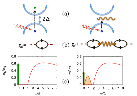
Figure 1: Schematic of the optical absorption $\sigma_{S}/\sigma_{N}$ (S=SC, N=normal state) in a disordered superconductor. In the BCS approach (left) only the single-particle excitations across the SC gap $2\Delta$ (a) are included, corresponding to the bare-bubble approximation (b) for the current-current response function. The resulting optical conductivity (c) consists of a delta peak at $\omega=0$ of weight $D_{s}^{BCS}$ (arrow) plus a regular part (solid line) starting at $\omega=2\Delta$. When vertex corrections are included (right) an excited quasiparticle can be converted in a collective mode (a), described in the diagrammatic approach (b) by the RPA resummations of the corresponding amplitude, phase or density fluctuations. An additional absorption appears at energies $\omega<2\Delta$ (c), corresponding to a superfluid peak at $\omega=0$ with strength $D_{s}<D_{s}^{BCS}$.

II Fermionic model

The model Hamiltonian we consider to investigate a disordered superconductor is the attractive Hubbard model ($U<0$) with local disorder $V_{i}\in[-V,V]$ and hopping $t$ restricted to nearest-neighbors,

$$H=-t\sum_{\langle ij\rangle\sigma}(c^{\dagger}_{i\sigma}c_{j\sigma}+h.c.)+U\sum_{i}n_{i\uparrow}n_{i\downarrow}+\sum_{i\sigma}V_{i}n_{i\sigma}$$ (1)

which we solve in mean-field on a $N\equiv N_{x}\times N_{y}$ lattice (up to $N=20\times 20$ with periodic boundary conditions) by using the BdG approachschrieffer ; degennes . The total current in direction $\alpha$ is defined as usual as:

$$J_{\alpha}({\bf q},\omega) = -e^{2}K_{\alpha\beta}({\bf q},\omega)A_{\beta}({\bf q},\omega),$$ (2)

$$K_{\alpha\beta}({\bf q},\omega) = D\delta_{\alpha\beta}-\chi_{\alpha\beta}({\bf q},\omega)\,.$$ (3)

Here $D=\frac{-t}{N}\sum_{n,\sigma}\Big{\langle}\big{(}c_{n,\sigma}^{\dagger}c_{n+\hat{\alpha}\sigma}+h.c.\big{)}\Big{\rangle}$ is the diamagnetic term, where $\langle\dots\rangle$ denotes the thermal and disorder average, which restores the translational invariance for model (1), allowing one to define the Fourier transform $\chi_{\alpha\beta}({\bf q},\omega)$ of the correlation function for the paramagnetic current $j_{n}^{\alpha}=-it\sum_{\sigma}\left[c_{n\sigma}^{\dagger}c_{n+\hat{\alpha},\sigma}-c^{\dagger}_{n+\hat{\alpha},\sigma}c_{n\sigma}\right]$. In a superconductor the superfluid stiffness is defined by the transverse ${\bf q}\rightarrow 0$ limit of Eq. (2). For example, for a field along the $x$ direction one has $J_{x}=-e^{2}D_{s}A_{x}$ where

$$D_{s} = D-\mathrm{Re}\,\chi_{xx}(q_{x}=0,q_{y}\rightarrow 0,\omega=0).$$ (4)

The optical conductivity is obtained from Eq. (2) by assuming a homogeneous vector potential, so that $A_{x}(\omega)=E_{x}(\omega)/i\omega$ and the real part of the optical conductivity is $\sigma(\omega)=-e^{2}\mathrm{Re}\,\frac{K_{xx}({\bf q}=0,\omega)}{i(\omega+i0^{+})}$, leading to

$$\sigma(\omega) = e^{2}\pi\delta(\omega)\left[D-\mathrm{Re}\,\chi_{xx}({\bf 0},\omega)\right]+e^{2}\frac{\mathrm{Im}\,\chi_{xx}({\bf 0},\omega)}{\omega}$$ (5)

$$\equiv e^{2}\pi D_{s}\delta(\omega)+\sigma_{reg}(\omega)$$

where we separeted explicitly the superfluid response at $\omega=0$ from the regular part $\sigma_{reg}$ occurring at finite frequency. By using the Kramers-Kronig relations for the $\chi_{xx}$ one then finds the well-know optical sum rule

$$\int_{0}^{\infty}d\omega\sigma(\omega)=\frac{\pi e^{2}}{2}D_{s}+\int_{0^{+}}^{\infty}\sigma_{reg}(\omega)=\frac{\pi e^{2}}{2}D.$$ (6)

The above Eq. (6) shows that any paramagnetic process described by $\sigma_{reg}$ leads to a suppression of the superfluid stiffness with respect to the diamagnetic term $D$, which at small density and weak interactions reduces to the usual form $D\simeq n/m$. In the BCS theory $\chi\equiv\chi_{0}$ is computed in the so-called bare-bubble approximation (see Fig. 1b, left)schrieffer , in which one includes only particle-hole excitations on top of the BCS ground state. At $T=0$ these excitations are exponentially suppressed by the opening of the gap, so that the optical absorption is possible only above the threshold to break a Cooper pair, i.e. at $\omega>\omega_{pair}=2\Delta$ (see Fig. 1c, left). Provided that $\omega_{pair}$ is smaller than the inverse lifetime of quasiparticles the resulting $\sigma^{BCS}_{reg}(\omega)$ is given by the well-known Mattis-Bardeen formulamattis , and the superfluid stiffness $D_{s}^{BCS}$ is smaller than $D$ already at $T=0$. In the following we will show that also collective modes, neglected in the BCS approach, give rise to a finite contribution to $\sigma_{reg}(\omega)$ at strong disorder, that is located mainly below $\omega_{pair}$ (see Fig. 1c, right). This additional optical absorption is accompanied by a further reduction of $D_{s}$ with respect to $D_{s}^{BCS}$ seibold12 , that has been experimentally reportedmondal11 ; driessen_prl12 ; driessen_prb13 .

The full optical response beyond BCS level can be computed by including vertex correctionsschrieffer , that also guarantee full gauge invariance of the theoryschrieffer ; nota_ea . The current-current correlation function $\chi$ can then be expressed in a compact form as (see App. A):

$$\chi=\chi_{0}+\hat{\Lambda}^{T}V[1-\hat{\Pi}^{0}V]^{-1}\hat{\Lambda}$$ (7)

where $\hat{\Lambda}$ is the vector containing the correlation functions that couple the current $j^{\alpha}_{n}$ to collective modes, i.e. particle-particle (amplitude and phase) and density fluctuations, described by the RPA resummation of the bare susceptibility $\hat{\Pi}^{0}$, see Fig. 1b right. The $\hat{V}$ and $\hat{\Pi}^{0}$ are matrices both in real space and in the phase space of collective modes, and translational invariance for $\chi$ is recovered after average over disorder configurations. In the clean case collective modes contribute only to the longitudinal response at finite ${\bf q}$ schrieffer ; nota_ea . In contrast, disorder renders the $\hat{\Lambda}$ susceptibilities finite even for a ${\bf q}=0$ external perturbation, so that the collective modes contribute to the optical response. Notice that this optical mechanism is similar to the one discussed recently for few-layer graphenefano-rice to explain the huge infrared-phonons peaksfano-exp . In that case doping activates the intermediate particle-hole process, analogously to what disorder does in our problem.

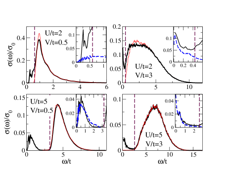
Figure 2: $\sigma(\omega)$ in units of $\sigma_{0}\equiv e^{2}/\hbar$ for the fermionic model (1). Here $N=$ and we averaged over … disorder configurations. The main panels report the curves without (thin, red) and with (thick, black) vertex corrections, while the dashed vertical lines mark $\omega_{pair}=2\Delta$. Insets: zoom of the low-energy part along with the results of the bosonic model (8) (dashed lines), with $W,J$ parameters assigned as described in the text.

The results for the optical conductivity at finite frequency for two representative values of coupling $U$ and disorder are shown in Fig. 2, along with their BCS counterparts. As one can see, the major differences between the two appear below the scale $\omega_{pair}=2\Delta$, marked with a dashed line. Notice that in the model (1) the spectral gap $\Delta$ in the single-particle excitations remains finite (and relatively large) at strong disorder, as it has been discussed previouslyranderia01 ; dubi07 ; randeria11 . As a consequence, the BCS calculation always shows a finite threshold at $\omega_{pair}$, with a profile that coincides at low disorder with the Mattis-Bardeen predictionmattis . In contrast, the full response extends also below $\omega_{pair}$, with a shape and intensity that depend both on the SC coupling $U$ and disorder. This result can explain the residual optical absorption in the microwave regimearmitage_prb07 ; frydman_cm13 and deviations from BCS theorymondal11 ; driessen_prl12 ; driessen_prb13 observed recently at strong disorder. In particular, the smearing of the $\omega_{pair}$ treshold due the presence of a dissipative channel associated to phase modes can lead to an apparent optical gap smaller than the one measured by STM, explaining the puzzling results of Ref. [frydman_cm13, ]. At the same time this effect can influence the performance of superconducting microwave devices, a field that has grown dramatically over the past decadezmuidzinas12 . Finally, two remarks are in order with respect to the results of Fig. 2. First of all, we checked that even though all the collective modes enter in the full response, the main contribution to $\sigma_{reg}(\omega)$ at low energy stems from phase fluctuations. This is shown explicitly in Fig. 3, where $\sigma_{reg}(\omega)$ has been computed by including only the phase-current vertex in Eq. 7 (see Appendix A). Second, one could wonder what happens when the Coulomb interaction, neglected in the present calculations, is taken into account. Indeed, one usually expects that the presence of long-range interactions the sound-like dispersion of phase modes is converted into a plasmonic one.nota_ea However, we do not expect that this result will spoil our conclusions: indeed, while plasmonic modes appear in the longitudinal response, the transverse optical response, which is the one discussed here, should be anyway screened, as shown explicitly in the weakly-disordered case in Ref. [belitz, ].

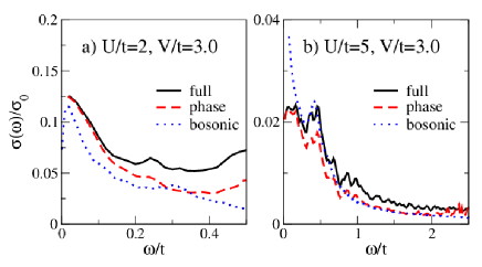
Figure 3: Comparison between $\sigma(\omega)$ computed using the full gauge-invariant response (solid line, black) and the contribution of phase fluctuations only (dashed line, red) (see Appendix A). The results of Fig. 2 for the bosonic model (8) (dotted line, blue) are reported as well.

III Bosonic model

To systematically address the structure of the phase excitations responsible for the sub-gap absorption we compute the optical conductivity also within an effective bosonic model for the disordered superconductor, i.e. the $XY$ spin 1/2 model in a transverse random fieldma_prb85 :

$$\mathcal{H}_{PS}\equiv-2\sum_{i}\xi_{i}S_{i}^{z}-2J\sum_{\langle i,j\rangle}\left(S^{+}_{i}S^{-}_{j}+h.c.\right).$$ (8)

In the pseudo-spin language $S^{z}=\pm 1/2$ corresponds to a site occupied or unoccupied by a Cooper pair, while superconductivity corresponds to a spontaneous in-plane magnetization, e.g. $\langle S^{x}_{i}\rangle\neq 0$. Disorder is represented by the random transverse field $\xi_{i}$, box distributed between $-W$ and $W$. The optical response of classicalstroud_prb00 and quantumranderia13 $XY$-like models has been addressed previously, by introducing disorder in the coupling $J$. The model (8) focuses instead on the competition between pair hopping ($J$) and localization ($W$)ma_prb85 ; fim_prb10 ; lemarie_prb13 ; laflorencie_prl13 , that has been recently proven successfullsacepe11 ; lemarie_prb13 to describe the STM experimental results in the SC phase near the SIT. We first solve the model (8) in mean-field to determine $\langle S^{x}_{i}\rangle=\frac{1}{2}\sin\theta_{i}$ and then rotate to the local coordinate system such that the new z-axis is $\widetilde{S_{i}^{z}}=S^{z}_{i}\cos\theta_{i}+S^{x}_{i}\sin\theta_{i}$. At strong disorder the SC order parameter develops an inhomogeneous spatial distribution, with SC islands embedded in an insulating background (cfr Fig. 6 below), in analogy both with the fermionic model (1)randeria01 ; dubi07 ; seibold12 and with tunnelling experimentssacepe11 ; pratap13 . Small fluctuations with respect to the mean-field configuration can be described by means of a Holstein-Primakov (HP) scheme, where spins are bosonized as usual as $\widetilde{S_{i}^{z}}=1/2-a^{+}_{i}a_{i}$, $\widetilde{S_{i}^{+}}\simeq a_{i}$ and $\widetilde{S_{i}^{-}}\simeq a^{+}_{i}$. Here we have defined $\widetilde{S_{i}^{\pm}}=\widetilde{S_{i}^{x}}\pm i\widetilde{S_{i}^{y}}$ with $\widetilde{S_{i}^{x}}=-S^{z}_{i}\sin\theta_{i}+S^{x}_{i}\cos\theta_{i}$ and $\widetilde{S_{i}^{y}}=S^{y}_{i}$ being orthogonal to the local quantization axis. The Hamiltonian (8) is then mapped into a quadratic model $\mathcal{H}_{PS}=E_{MF}+\mathcal{H}^{\prime}_{PS}$ that can be diagonalized by means of a Bogoliubov transformation $a_{i}=\sum_{\alpha}\left(u_{\alpha i}\gamma_{\alpha}+v_{\alpha i}\gamma^{\dagger}_{\alpha}\right)$:

$$\mathcal{H}^{\prime}_{PS} = \sum_{ij}\left[A_{ij}(a^{\dagger}_{i}a_{j}+h.c.)+\frac{1}{2}B_{ij}\left(a_{i}a_{j}+h.c.\right)\right]$$ (9)

$$= \sum_{\alpha}E_{\alpha}\gamma^{\dagger}_{\alpha}\gamma_{\alpha}+const.$$

Here $A_{ij}=2\delta_{ij}\xi_{i}/\cos\theta_{i}-J(1+\cos\theta_{i}\cos\theta_{j})(1-\delta_{ij})$ and $B_{ij}=J(1-\cos\theta_{i}\cos\theta_{j})(1-\delta_{ij})$ are the matrices that enter in the eigenvalue problem for the excitation energies $E_{\alpha}$nota_gm . The equivalence between the HP excitations and the SC phase excitations at Gaussian level can be made explicit by the identification of the phase operators $\Phi_{i}$ and their conjugated momenta $L_{i}$,

$$\Phi_{i} = -2\frac{S^{y}_{i}}{\sin\theta_{i}}=\sum_{\alpha}i\frac{\phi_{\alpha i}}{\sqrt{2}}(\gamma_{\alpha}^{\dagger}-\gamma_{\alpha}),$$ (10)

$$L_{i} = S_{i}^{\perp}\sin\theta_{i}=\sum_{\alpha}\frac{\ell_{\alpha i}}{\sqrt{2}}(\gamma_{\alpha}^{\dagger}+\gamma_{\alpha}),$$ (11)

where $\phi_{\alpha i}=\sqrt{2}\left(v_{\alpha i}-u_{\alpha i}\right)/\sin\theta_{i}$ and $\ell_{\alpha i}=\left(u_{\alpha i}+v_{\alpha i}\right)\sin\theta_{i}/\sqrt{2}$. The fluctuation part of the Hamiltonian (9) can then be expressed as:

$${\cal H}^{\prime}_{PS}=\frac{1}{2}\sum_{i,\mu=x,y}J^{\mu}_{i}\left[\Delta_{\mu}\Phi_{i}\right]^{2}+\frac{1}{2}\sum_{ij}{\cal X}^{-1}_{ij}L_{i}L_{j}$$ (12)

where $J^{\mu}_{i}\equiv J\sin\theta_{i}\sin\theta_{i+\hat{\mu}}$ are the local stiffnesses of the disordered superconductor, $\Delta_{\mu}$ is the discrete derivative in the $\mu$ direction and ${\cal X}^{-1}_{ij}=2(A_{ij}+B_{ij})/\sin\theta_{i}\sin\theta_{j}$ is the inverse matrix of the compressibilities. Consistently with the identification (10) the usual Peierls coupling to the gauge field in the pseudospin model (8) corresponds to the replacement $S^{+}_{i}S^{-}_{i+\mu}\rightarrow S^{+}_{i}S^{-}_{i+\mu}e^{-2ieA_{\mu}}$, with a factor of 2 accounting for the double charge of each Cooper pair. This leads in Eq. (12) to the shift $\Delta_{\mu}\Phi_{i}\rightarrow\Delta_{\mu}\Phi_{i}-2eA_{\mu}$, i.e. the usual minimal-coupling scheme. The real part of the optical conductivity for the bosonic model (8) is then easily obtained as $\sigma^{B}(\omega)=e^{2}\pi\delta(\omega)D^{B}_{s}+\sigma_{reg}^{B}(\omega)$ with

$$D_{s}^{B} = D^{B}-\frac{1}{N}\sum_{\alpha}Z_{\alpha}$$ (13)

$$\sigma_{reg}^{B}(\omega) = \frac{e^{2}\pi}{2N}\sum_{\alpha}Z_{\alpha}\left[\delta(\omega+E_{\alpha})+\delta(\omega-E_{\alpha})\right],$$ (14)

where $D^{B}=(1/N)\sum_{i}4J^{\mu}_{i}$ is the diamagnetic term of the bosonic model (8), $\mu=x$ for instance and the effective dipole $Z_{\alpha}$ of each excitation mode is

$$Z_{\alpha}=\frac{1}{E_{\alpha}}\left[\sum_{i}2J_{i}^{\mu}\Delta_{\mu}\phi_{\alpha i}\right]^{2}.$$ (15)

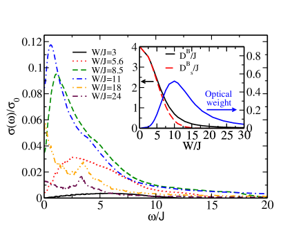
Figure 4: $\sigma_{reg}(\omega)/\sigma_{0}$ for the bosonic model (8) at different values of $W/J$. The lattice size is $N=50\times 50$ and the average is taken over 100 disorder configurations. Inset: disorder dependence of the diamagnetic term $D^{B}$, the superfluid stiffness $D_{s}^{B}$ and the total spectral weight $\int_{0^{+}}^{\infty}d\omega\sigma_{reg}(\omega)=(\pi/2)(D^{B}-D_{s}^{B})$ in units of $J$.

For a uniform stiffness ($J_{i}^{\mu}=$const) one finds that $Z_{\alpha}$ is proportional to the total derivative of the phase modulation, which then vanishes for periodic boundary conditions. Thus, the inhomogeneity of $J^{\mu}_{i}$ induced by disorder is a crucial prerequisite to obtain a finite electric dipole, responsible for the $\sigma_{reg}(\omega)$ shown in Fig. 4. As one can see, the optical response moves towards decreasing energies for increasing disorder (i.e. $W/J$), and its total spectral weight $\int_{0^{+}}^{\infty}d\omega\sigma_{reg}(\omega)=(\pi/2)(D^{B}-D^{B}_{s})$ [see Eq. (13)-(14)] first increases, due to the disorder-tuned optical absorption at finite $\omega$, and then decreases again, due to the strong suppression by disorder of the diamagnetic term $D^{B}$ itself (see inset Fig. 4). Notice that the decrease of $D^{B}$ with increasing disorder reflects the suppression of the local order parameter, encoded in the fermionic language (1) in the suppression of the BCS stiffness $D_{s}^{BCS}$. This analogy can be used to obtain a quantitative comparison between the fermionic and the bosonic approach, by fixing $W/J$ of the model (8) in order to reproduce $D^{B}_{s}/D^{B}=D_{s}/D_{s}^{BCS}$. In this way we can account in both models for the same transfer of spectral weight from $\omega=0$ to $\sigma_{reg}(\omega)$ (see Appendix B). The results are shown in the insets of Fig. 2 and in Fig. 3: as one can see, at large $U$ the bosonic model reproduces in a quantitative way the characteristic energy scales for optical absorption in the fermionic model. At weaker coupling the comparison is instead only qualitative, due partly to the difficulties of clearly separating the contribution of quasiparticles and collective modes.

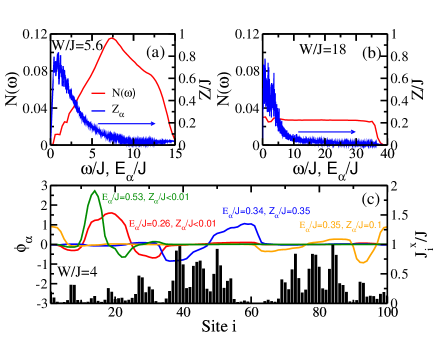
Figure 5: (a)-(b) Density of phase modes $N(\omega)$ and effective dipole $Z_{\alpha}$ at two values of disorder (averaged over 100 disorder configurations). (c) Spatial structure of the phase modes in the one-dimensional case at selected energies for a given disorder realization, along with the spatial variations of the stiffness $J_{i}^{x}$, represented with bars. The largest effective dipole is realized for the blue and orange excitations, whose monotonic phase variations overlap with a region of large local stiffness.

Let us finally analyze the connection between the optical response and the inhomogeneous spatial distribution of the SC properties. The optical response (14) is proportional to the density of states of phase modes $N(\omega)$, weighted by the effective dipole function $Z_{\alpha}$ of Eq. (15). Both quantities depend on disorder, as it is shown in Fig. 5a,b, and in general the $1/E_{\alpha}$ prefactor of Eq. (15) favors a larger dipole for lower-energy modes. In addition at strong disorder, when the system segregates into SC islands with large local stiffness $J_{\mu}^{i}$, the optical absorption is large when the phase excitations occur inside the SC regions, according to Eq. (15). This effect can be better visualized in a one-dimensional version of the model (8), as it is shown in panel (c) of Fig. 5. Here one can clearly see that the largest optical dipole is realized when a monotonic phase variation overlaps with a good SC region. Since the charge is the conjugate variable of the phase gradients, one then realizes a charge unbalance on the two sides of the island, making it optically active.

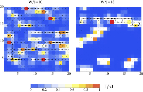
Figure 6: Local supercurrents (arrows) for an applied field ${\bf A}=-A\hat{x}$ superimposed over the map of the local stiffnesses $J_{i}^{x}/J$ for a given disorder realization and two values of $W/J$. The size of the arrows is proportional to the strenght of the total local current, whose diamagnetic contribution is proportional to the local stiffness displayed in the underlying map. The current flows along preferential paths connecting the regions with large $J_{i}^{x}$. This means that the isolated SC islands, i.e. those which reside far from the main percolative paths of the current, have a large paramagnetic response responsible for the absorption at finite frequencies. For example, for $W/J=18$ all the diamagnetic contribution of the white regions on the bottom of the map is transferred to $\sigma_{reg}(\omega)$.

At strong disorder this space-selective optical absorption is strictly connected to the emergence of percolative paths for the superfluid currents, analogous to the ones discussed in Ref. [seibold12, ] for the fermionic model (1). In Fig. 6 we show at two values of $W/J$ the currents in the presence of a finite applied field ${\bf A}=-A\hat{x}$ for a given disorder configuration, superimposed to the map of the local stiffnessess $J_{i}^{x}$. Since $J_{i}^{x}$ is a measure of the local diamagnetic response, a small current occurring over a good SC region is due to a large local paramagnetic response, i.e. to an optical absorption at finite frequencies. At strong disorder the percolative supercurrent paths leave aside several isolated SC islands, which then contribute to $\sigma_{reg}(\omega)$ thanks to the dipole-activation mechanism explained above.

IV Conclusions

In summary, we computed the optical response due to collective modes in two prototype fermionic and bosonic models for disordered superconductors. In both cases we find that disorder renders phase fluctuations optically active, in a range of energies that lies below the threshold for single-particle excitations for the fermionic case. The bosonic approach allows us to establish a clear correspondence between the optical response and the spatial inhomogeneity of the SC order parameter, showing that optical absorption stems predominantly from phase fluctuations within the good SC regions. Besides explaining recent experiments in strongly-disordered superconductorsarmitage_prb07 ; frydman_cm13 ; driessen_prl12 ; driessen_prb13 our results could be further checked experimentally by means of near-field scanning microwave impedance microscopyshen_nano09 . Indeed, the proposed mechanism of direct correspondence between the SC granularity and optical absorption, evidenced in Fig. 6, can be potentially mapped out by this technique, able to resolve spatial variations at length scales well below the radiation wavelength. In this respect the variation of the microwave optical properties of disordered superconductors at the nanoscale can be used to improve the performance of SC microresonators built in standard geometries, or even to design new nano-electric devices targeted for space- and frequency-selective applications.

We thank E. Driessen, A. Frydman and D. Sherman for useful discussions. L.B. acknowledges financial support by MIUR under Grant No. FIRB2012 (RBFR1236VV).

Appendix A Optical conductivity for the fermionic model

In order to compute fluctuations on top of the inhomogeneous BdG ground state we evaluate dynamical correlation functions

$$\chi_{nm}(\hat{X},\hat{Y})=-i\int\!dte^{i\omega t}\langle{\cal T}\hat{X}_{n}(t)\hat{Y}_{m}(0)\rangle$$ (16)

where $\hat{X}$,$\hat{Y}$ correspond to either pair or charge fluctuation operators, i.e. $\delta\Delta_{i}\equiv c_{i\downarrow}c_{i\uparrow}-\langle c_{i\downarrow}c_{i\uparrow}\rangle_{0}$, $\delta\Delta_{i}^{\dagger}\equiv c^{\dagger}_{i\uparrow}c^{\dagger}_{i\downarrow}-\langle c^{\dagger}_{i\uparrow}c^{\dagger}_{i\downarrow}\rangle_{0}$ and $\delta n_{i}\equiv\sum_{\sigma}\left(c^{\dagger}_{i\sigma}c_{i\sigma}-\langle c^{\dagger}_{i\sigma}c_{i\sigma}\rangle_{0}\right)$. Here and in the following a nought sub- or superscript denotes evaluation in the BdG ground state.

The local interactions between pair ($U\delta\Delta_{i}^{\dagger}\delta\Delta_{i}$, $U\delta\Delta_{i}\delta\Delta_{i}^{\dagger}$) and charge ($U/2\delta n_{i}\delta n_{i}$) fluctuations are contained in the matrix $\underline{\underline{V}}$ so that the resummation

$$\underline{\underline{\chi}}=\left[\underline{\underline{1}}-\underline{\underline{\chi^{0}}}\underline{\underline{V}}\right]^{-1}\underline{\underline{\chi^{0}}}$$ (17)

allows to compute the dynamical amplitude $A_{i}\equiv(\delta\Delta_{i}+\delta\Delta^{\dagger}_{i})/\sqrt{2}$ and phase $\Phi_{i}\equiv(\delta\Delta_{i}-\delta\Delta^{\dagger}_{i})/\sqrt{2}$ correlations.

Vertex corrections to the bare current-current correlation function $\chi^{0}_{nm}(j^{\alpha},j^{\beta})$ can be obtained by defining $\Lambda_{nm}^{\alpha}=\chi^{0}_{nm}(j^{\alpha},\hat{Y})$ and $\overline{\Lambda}_{mn}^{\alpha}=\chi^{0}_{mn}(\hat{Y},j^{\alpha})$ which couple the current $j^{\alpha}_{n}$ between sites $R_{n}$ and $R_{n+\hat{\alpha}}$ to the pair and charge fluctuations $\hat{Y}_{m}\equiv(A_{m},\Phi_{m},\delta n_{m})$. The full (gauge invariant) current correlation function is then obtained from

$$\chi_{nm}(j^{\alpha}_{n},j^{\beta}_{m}) = \chi^{0}_{nm}(j^{\alpha}_{n},j^{\beta}_{m})+\Lambda_{nm}^{\alpha}V_{mk}\overline{\Lambda}_{km}^{\beta}$$ (18)

$$+ \Lambda_{nm}^{\alpha}V_{mk}\chi_{kl}V_{ls}\overline{\Lambda}_{sm}^{\beta}$$

$$= \chi^{0}_{nm}(j^{\alpha}_{n},j^{\beta}_{m})$$

$$+ \Lambda_{nm}^{\alpha}V_{mk}\left[\underline{\underline{1}}-\underline{\underline{\chi^{0}}}\underline{\underline{V}}\right]^{-1}_{kl}\overline{\Lambda}_{lm}^{\beta}\,.$$

The average over several disorder configurations (typically $50-70$) restores translational invariance for $\chi_{nm}$, so that $\sigma(\omega)$ can be computed according to Eq. (5). The predominant role of phase fluctuations for the subgap optical response is demonstrated in Fig. 3. Here the dashed lines correspond to $\sigma(\omega)$ computed by including only the phase-current vertex in Eq. 18, whereas the solid lines correspond to the full optical conductivity, dressed by all the collective modes.

Appendix B Comparison between the bosonic and fermionic model

In order to make a quantitative comparison between the bosonic and fermionic models we propose a scheme based on the equivalence of the optical spectral weight due to collective modes in both models. In the fermionic model the diamagnetic term $D$ is only weakly dependent on disorder. On the other hand, the BCS estimate of the superfluid density $D_{s}^{BCS}$ is strongly suppressed due to the enhanced paramagnetic contribution of quasiparticles. In the bosonic model quasiparticle excitations are not present: however, the localization effects due to disorder are taken into account in the effective local stiffnesses $J_{i}^{\mu}$, which enter in the bosonic diamagnetic term $D^{B}$. Any additional correction due to phase fluctuations is encoded in the ratio $D_{s}/D_{s}^{BCS}$ or $D^{B}_{s}/D^{B}$ for the fermionic or bosonic model, respectively. The ratio $D_{s}/D_{s}^{BCS}$ measures also the relative strength of the sub-gap optical response with respect to the BCS-like part. However, since this one is also slightly modified by vertex corrections, especially at weak coupling (see red and black lines in Fig. 2), we estimate an effective $\tilde{D}_{s}^{BCS}$ from the integrated spectral weight at $\omega>2\Delta$ of the full optical conductivity. Thus, for a given $U$ in the fermionic model (1) we determine $W/J$ in the bosonic model (8) in order to have $D^{B}_{s}/D^{B}=D_{s}/\tilde{D}_{s}^{BCS}$. This establishes a rescaling function $\alpha$ such that $W/J=\alpha(V_{0}/t)$. We then fix a factor $\gamma$ ($J=\gamma t$) such that $D^{B}/J=\tilde{D}_{s}^{BCS}/\gamma t$, and we then plot $\sigma_{reg}$ as a function of $\omega/t$ as shown in the insets of Fig. 2. This procedure reveals that already for $U/t=5$, i.e in the intermediate-coupling regime, the ratio $J/t$ obtained in this way is very similar to the value $J/t\sim t/U$ predicted by the exact mapping of the clean attractive Hubbard model onto the pseudospin modelmicnas_prb81 .

References

- (1) For a review see e.g. P.A. Lee, N. Nagaosa, and X.-G. Wen, Rev. Mod. Phys. 78, 17 (2006).
- (2) K. K. Gomes, A. N. Pasupathy, A. Pushp, S. Ono, Y. Ando, and A. Yazdani, Nature 447, 569 (2007).
- (3) B.Sacépé, C. Chapelier, T. I. Baturina, V. M. Vinokur, M. R. Baklanov, M. Sanquer, Nature Communications 1, 140 (2010).
- (4) M. Mondal, A. Kamlapure, M. Chand, G. Saraswat, S. Kumar, J. Jesudasan, L. Benfatto, V. Tripathi, and P. Raychaudhuri, Phys. Rev. Lett. 106, 047001, (2011).
- (5) B. Sacépé, T. Dubouchet, C. Chapelier, M. Sanquer, M. Ovadia, D. Shahar, M. Feigel’man, and L. Ioffe, Nature Phys. 7, 239 (2011).
- (6) M. Chand, Garima Saraswat, Anand Kamlapure, Mintu Mondal, Sanjeev Kumar, John Jesudasan, Vivas Bagwe, Lara Benfatto, Vikram Tripathi, Pratap Raychaudhuri, Phys. Rev. B85, 014508 (2012).
- (7) Y. Noat, T. Cren, C. Brun, F. Debontridder, V. Cherkez, K. Ilin, M. Siegel, A. Semenov, H.-W. Hübers, D. Roditchev, Phys. Rev. B88, 014503 (2013).
- (8) Anand Kamlapure,Tanmay Das, Somesh Chandra Ganguli, Jayesh B. Parmar, Somnath Bhattacharyya and Pratap Raychaudhuri, Sci. Rep. 3, 2979 (2013).
- (9) C. Richter, H. Boschker, W. Dietsche, E. Fillis-Tsirakis, R. Jany, F. Loder, L. F. Kourkoutis, D. A. Muller, J. R. Kirtley, C. W. Schneider and J. Mannhart, Nature 502, 528 (2013).
- (10) Actually the origin of the pseudogap in underdoped cuprate superconductors is still an open problem, since it may also involve a second energy scale originating from a competing order (cf. Ref. gomes07 ).
- (11) A. Ghosal, M. Randeria and N. Trivedi, Phys. Rev. B65, 014501 (2001).
- (12) Y Dubi, Y. Meir and Y. Avishai, Nature 449, 876 (2007).
- (13) Y Dubi, Y. Meir and Y. Avishai, Phys. Rev. B78, 024502 (2008).
- (14) A.Erez and Y.Meir, Europhys. Lett. 91, 47003 (2010).
- (15) K. Bouadim, Y. L. Loh, M. Randeria and N. Trivedi, Nature Physics 7, 884 (2011).
- (16) G. Seibold, L. Benfatto, C. Castellani and J. Lorenzana, Phys. Rev. Lett. 108, 207004 (2012).
- (17) R. W. Crane, N. P. Armitage, A. Johansson, G. Sambandamurthy, D. Shahar, and G. Grüner, Phys. Rev. Lett. 75, 75, 094506 (2007).
- (18) D. Sherman, B. Gorshunov, S. Poran, J. Jesudasan, P. Raychaudhuri, N. Trivedi, M. Dressel, and A. Frydman, arXiv:1304.7087.
- (19) M. Ma and P. A. Lee, Phys. Rev. B 32, 5658 (1985).
- (20) S. Robaszkiewicz, R. Micnas, and K. A. Chao, Phys. Rev. B23, 1447 (1981).
- (21) K. Lai, H. Peng, W. Kundhikanjana, D. T. Schoen, C. Xie, S. Meister, Y. Cui, M. A. Kelly, and Z.-X. Shen, Nano Lett. 9, 1265 (2009).
- (22) J. Zmuidzinas, Annu. Rev. Condens. Matter Phys. 3 169, 2012.
- (23) R. S. Schrieffer, Theory of Superconductivity; Addison-Wesley (1964).
- (24) P.G. de Gennes, Superconductivity of Metals and Alloys, Westview Press (1966)
- (25) D. C. Mattis and J. Bardeen, Phys. Rev. 111, 412 (1958).
- (26) E. F. C. Driessen, P. C. J. J. Coumou, R. R. Tromp, P. J. de Visser, and T. M. Klapwijk, Phys. Rev. Lett. 109, 107003 (2012).
- (27) For a discussion of this issue within an effective-action formalism see e.g. A. Paramekanti, M. Randeria, T.V. Ramakrishnan, and S.S. Mandhal, Phys. Rev. B 62, 6786 (2000); L. Benfatto, A. Toschi and S. Caprara, Phys. Rev. B69, 184510 (2004); H. Guo, C.-C. Chien and Y. He, J. Low Temp. Phys. bf 172, 5 (2013).
- (28) E. Cappelluti, L. Benfatto, M. Manzardo, and A. B. Kuzmenko, Phys. Rev. B 86, 115439 (2012).
- (29) A. B. Kuzmenko, L. Benfatto, E. Cappelluti, I. Crassee, D. van der Marel, P. Blake, K. S. Novoselov, A. K. Geim, Phys. Rev. Lett. 103, 116804 (2009); Z. Li, C.-H. Lui, E. Cappelluti, L. Benfatto, K.-F. Mak, G. L. Carr, J.Shan, T. F. Heinz, Phys. Rev. Lett. 108, 156801 (2012).
- (30) P. C. J. J. Coumou1, E. F. C. Driessen, J. Bueno, C. Chapelier, and T. M. Klapwijk, Phys. Rev. B88, 180505(R) (2013).
- (31) D. Belitz, S. De Souza-Machado, T. P. Deveraux and D. W. Hoard, Phys. Rev. B39, 2072 (1989).
- (32) S. Barabash, D. Stroud and I.-J. Hwang, Phys. Rev. B61, R14924 (2000); S. Barabash and D. Stroud, Phys. Rev. B67, 144506 (2003).
- (33) M.Swanson, Y.-L. Loh, M. Randeria and N. Trivedi, arXiv:1310.1073.
- (34) L. B. Ioffe and M. Mezard Phys. Rev. Lett. 105, 037001 (2010); M. V. Feigel’man, L. B. Ioffe, and M. Mézard Phys. Rev. B82, 184534 (2010).
- (35) G. Lemarié, A. Kamlapure, D. Bucheli, L. Benfatto, J. Lorenzana, G. Seibold, S. C. Ganguli, P. Raychaudhuri, and C. Castellani, Phys. Rev. B 87, 079904 (2013).
- (36) Juan Pablo Álvarez Zúniga and N. Laflorencie, Phys. Rev. Lett. 111, 160403 (2013).
- (37) We verified that the first eigenvalue always corresponds to a zero-energy mode, as expected for the limit of the Goldstone mode of the symmetry broken in the SC phase.