Power Allocation in MIMO Wiretap Channel with Statistical CSI and Finite-Alphabet Input

Abstract

In this paper, we consider the problem of power allocation in MIMO wiretap channel for secrecy in the presence of multiple eavesdroppers. Perfect knowledge of the destination channel state information (CSI) and only the statistical knowledge of the eavesdroppers CSI are assumed. We first consider the MIMO wiretap channel with Gaussian input. Using Jensen’s inequality, we transform the secrecy rate max-min optimization problem to a single maximization problem. We use generalized singular value decomposition and transform the problem to a concave maximization problem which maximizes the sum secrecy rate of scalar wiretap channels subject to linear constraints on the transmit covariance matrix. We then consider the MIMO wiretap channel with finite-alphabet input. We show that the transmit covariance matrix obtained for the case of Gaussian input, when used in the MIMO wiretap channel with finite-alphabet input, can lead to zero secrecy rate at high transmit powers. We then propose a power allocation scheme with an additional power constraint which alleviates this secrecy rate loss problem, and gives non-zero secrecy rates at high transmit powers.

keywords: MIMO wiretap channel, physical layer security, secrecy rate, multiple eavesdroppers, statistical CSI, finite-alphabet input.

I Introduction

Wireless transmissions are vulnerable to eavesdropping due to their broadcast nature. There is a growing demand to address the issue of providing security in wireless networks. Secrecy in wireless communication networks can be achieved using physical layer techniques, where the legitimate receiver gets the transmitted information correctly and the eavesdropper receives no or very little information. Achievable secrecy rates and secrecy capacity bounds for multiple antenna point-to-point wiretap channel has been studied in [1, 2, 3, 4]. In [1], [5], multiple-input single-output (MISO) wiretap channel is considered, and secrecy rate is computed assuming statistical information of the eavesdropper channel. In [6], [7], secrecy capacity of the multiple-input multiple-output (MIMO) wiretap channel has been computed assuming perfect channel state information (CSI) knowledge of the destination and the eavesdropper. These works consider secrecy rate when the input to the channel is Gaussian. In practice, the input to the channel will be from a finite alphabet set, e.g., $M$-ary alphabets. The effect of finite-alphabet input on the achievable secrecy rate for various channels has been studied in [8, 9, 10, 11]. It has been shown that with finite-alphabet input, increasing the power beyond a maximum point is harmful as the secrecy rate curve dips continuously thereafter. In [12], design of optimum linear transmit precoding for maximum secrecy rate over MIMO wiretap channel with finite-alphabet input and with perfect eavesdropper CSI assumption has been investigated.

In this paper, we consider the problem of power allocation in MIMO wiretap channel for secrecy in the presence of multiple eavesdroppers. To our knowledge, such a study for the case of finite-alphabet input when only the statistical CSI of the eavesdroppers is assumed has not been reported before. Our approach to study this problem, which is adopted in this paper, is summarized as follows. First, we consider the MIMO wiretap channel with Gaussian input and knowledge of statistical CSI of the eavesdroppers. We transform the secrecy rate max-min optimization problem with Gaussian input into a single maximization problem using Jensen’s inequality. Generalized singular value decomposition (GSVD) is used to transform the problem to a concave maximization problem which maximizes the sum secrecy rate of scalar wiretap channels subject to linear constraints on the transmit covariance matrix. We then consider the MIMO wiretap channel with finite-alphabet input and knowledge of statistical CSI of the eavesdroppers. It is found that when the transmit covariance matrix obtained for the case of Gaussian input is used in the MIMO wiretap channel with finite-alphabet input, the secrecy rate goes to zero at high transmit powers. Therefore, we propose a power allocation scheme with an additional power constraint to deal with this secrecy rate loss. The proposed scheme is shown to alleviate the secrecy rate loss problem and gives non-zero secrecy rates at high transmit powers.

The rest of the paper is organized as follows. The system model is presented in Section II. The secrecy rate with Gaussian input is studied in Section III. The secrecy rate with finite-alphabet input is studied in Section IV. Numerical results and conclusions are presented in Section V and Section VI, respectively.

$\bf{Notations:}$ Vectors are denoted by boldface lower case letters, and matrices are denoted by boldface upper case letters. $\boldsymbol{A}\in\mathbb{C}^{N_{1}\times N_{2}}$ implies that $\boldsymbol{A}$ is a complex matrix of dimension $N_{1}\times N_{2}$. $\boldsymbol{A}\succeq\boldsymbol{0}$ denotes that $\boldsymbol{A}$ is a positive semidefinite matrix. $\boldsymbol{I}$ denotes the identity matrix. Transpose and complex conjugate transpose operations are denoted with $[.]^{T}$ and $[.]^{\ast}$, respectively. $diag(\boldsymbol{a})$ denotes a diagonal matrix with elements of vector $\boldsymbol{a}$ on the diagonal of the matrix. $diag(\boldsymbol{A})$ denotes a vector formed with the diagonal entries of matrix $\boldsymbol{A}$. $\mathbb{E}\big{[}.\big{]}$ denotes expectation operation.

II System Model

Consider a MIMO wiretap channel which consists of a source $S$, an intended destination $D$, and $J$ eavesdroppers {$E_{1},E_{2},\cdots,E_{J}$}. The system model is shown in Fig. 1. Source $S$ has $N_{S}$ transmit antennas, destination $D$ has $N_{D}$ receive antennas and each eavesdropper $E_{j}$ has $N_{E_{j}}$ receive antennas. The complex fading channel gain matrix between $S$ to $D$ is denoted by $\boldsymbol{H}\in\mathbb{C}^{N_{D}\times N_{S}}$. Likewise, the channel gain matrix between $S$ to $E_{j}$ is denoted by $\boldsymbol{Z}_{j}\in\mathbb{C}^{N_{E_{j}}\times N_{S}}$. We assume that the channel gain matrix, $\boldsymbol{H}$, between $S$ to $D$ is known perfectly. We also assume that the channel gains of all the eavesdroppers are unknown and that all the channel gains of eavesdroppers are i.i.d $\sim\mathcal{CN}(0,\sigma^{2}_{E_{j}})$.

Figure 1: System model.

Let $P_{0}$ denote the total available transmit power. The source $S$ transmits the complex vector symbol $\boldsymbol{x}\sim\mathcal{CN}(\boldsymbol{0},\boldsymbol{Q})$, where $\boldsymbol{Q}=\mathbb{E}\{\boldsymbol{x}\boldsymbol{x}^{\ast}\}$ is the transmit covariance matrix and $trace(\boldsymbol{Q})\leq P_{0}$. Let $\boldsymbol{y}_{D}$ and $\boldsymbol{y}_{E_{j}}$ denote the received signals at the destination $D$ and the $j$th eavesdropper $E_{j}$, respectively. We then have

$$\boldsymbol{y}_{D}=\boldsymbol{H}\boldsymbol{x}+\boldsymbol{\eta}_{D},$$ (1)

$$\boldsymbol{y}_{E_{j}}=\boldsymbol{Z}_{j}\boldsymbol{x}+\boldsymbol{\eta}_{E_{j}},$$ (2)

where $\boldsymbol{\eta}_{D}\sim\mathcal{CN}(\boldsymbol{0},N_{0}\boldsymbol{I})$ and $\boldsymbol{\eta}_{E_{j}}\sim\mathcal{CN}(\boldsymbol{0},N_{0}\boldsymbol{I})$ are the i.i.d. noise vectors at $D$ and $E_{j}$, respectively.

III MIMO Wiretap Channel with Gaussian Input

For a given $\boldsymbol{H}$, using (1), the information rate at the destination $D$ is

$$I(\boldsymbol{x};\ \boldsymbol{y}_{D})=\log_{2}\det\Big{(}\boldsymbol{I}+\frac{\boldsymbol{H}\boldsymbol{Q}\boldsymbol{H}^{\ast}}{N_{0}}\Big{)}.$$ (3)

Similarly, for a given $\boldsymbol{Z}_{j}$, using (2), the information rate at the $j$th eavesdropper $E_{j}$, $\forall j=1,2,\cdots,J,$ is

$$I(\boldsymbol{x};\ \boldsymbol{y}_{E_{j}})=\log_{2}\det\Big{(}\boldsymbol{I}+\frac{\boldsymbol{Z}_{j}\boldsymbol{Q}\boldsymbol{Z}^{\ast}_{j}}{N_{0}}\Big{)}.$$ (4)

Subject to the total power constraint $P_{0}$, using (3) and (4), the secrecy rate $R_{s}$ for the MIMO wiretap channel is obtained by solving the following optimization problem [1], [5]:

$$R_{s}\ =\ \max_{\boldsymbol{Q}}\ \min_{j:1,2,\cdots,J}\bigg{\{}\log_{2}\det\Big{(}\boldsymbol{I}+\frac{\boldsymbol{H}\boldsymbol{Q}\boldsymbol{H}^{\ast}}{N_{0}}\Big{)}-$$

$$\mathbb{E}\bigg{[}\log_{2}\det\Big{(}\boldsymbol{I}+\frac{\boldsymbol{Z}_{j}\boldsymbol{Q}\boldsymbol{Z}^{\ast}_{j}}{N_{0}}\Big{)}\bigg{]}\bigg{\}},$$ (5)

$$\geq\ \max_{\boldsymbol{Q}}\ \min_{j:1,2,\cdots,J}\ \bigg{\{}\log_{2}\det\Big{(}\boldsymbol{I}+\frac{\boldsymbol{H}\boldsymbol{Q}\boldsymbol{H}^{\ast}}{N_{0}}\Big{)}-$$

$$\log_{2}\det\Big{(}\boldsymbol{I}+\frac{N_{E_{j}}\sigma^{2}_{E_{j}}\boldsymbol{Q}}{N_{0}}\Big{)}\bigg{\}},$$ (6)

$$=\ \max_{\boldsymbol{Q}}\ \bigg{\{}\log_{2}\det\Big{(}\boldsymbol{I}+\frac{\boldsymbol{H}\boldsymbol{Q}\boldsymbol{H}^{\ast}}{N_{0}}\Big{)}-$$

$$\log_{2}\det\Big{(}\boldsymbol{I}+\frac{N_{E_{j_{0}}}\sigma^{2}_{E_{j_{0}}}\boldsymbol{Q}}{N_{0}}\Big{)}\bigg{\}},$$ (7)

$$=\ \max_{\boldsymbol{Q}}\ \bigg{\{}\log_{2}\det\Big{(}\boldsymbol{I}+\frac{\boldsymbol{H}\boldsymbol{Q}\boldsymbol{H}^{\ast}}{N_{0}}\Big{)}-$$

$$\log_{2}\det\Big{(}\boldsymbol{I}+\frac{\boldsymbol{Z}\boldsymbol{Q}\boldsymbol{Z}^{\ast}}{N_{0}}\Big{)}\bigg{\}},$$ (8)

$$\text{s.t.}\quad\boldsymbol{Q}\ \succeq\ \boldsymbol{0},\quad trace(\boldsymbol{Q})\ \leq\ P_{0},$$ (9)

where (6) is written using Jensen’s inequality, $j_{0}$ in (7) corresponds to the eavesdropper with maximum $N_{E_{j_{0}}}\sigma^{2}_{E_{j_{0}}}$, and $\boldsymbol{Z}$ in (8) is $\sqrt{N_{E_{j_{0}}}\sigma^{2}_{E_{j_{0}}}}\boldsymbol{I}$. We intend to find the $\boldsymbol{Q}$ which maximizes the objective function in (8) subject to the constraints in (9). To do this, we take the GSVD [13] of $\boldsymbol{H}$ and $\boldsymbol{Z}$ as

$$\boldsymbol{H}\ =\ \boldsymbol{U}\boldsymbol{\Lambda_{\boldsymbol{H}}}\Big{[}\boldsymbol{\Phi}^{\ast}\boldsymbol{T},\ \boldsymbol{0}\Big{]}\boldsymbol{W}^{\ast}$$ (10)

$$\boldsymbol{Z}\ =\ \boldsymbol{V}\boldsymbol{\Lambda_{\boldsymbol{Z}}}\Big{[}\boldsymbol{\Phi}^{\ast}\boldsymbol{T},\ \boldsymbol{0}\Big{]}\boldsymbol{W}^{\ast}.$$ (11)

$\boldsymbol{U}$, $\boldsymbol{V}$, $\boldsymbol{\Phi}$, and $\boldsymbol{W}$ are unitary matrices of dimensions $N_{D}\times N_{D}$, $N_{S}\times N_{S}$, $k\times k$, and $N_{S}\times N_{S}$, respectively. $\boldsymbol{T}$ is an upper triangular matrix of size $k\times k$ and rank-$k$. $\boldsymbol{\Lambda_{\boldsymbol{H}}}$ and $\boldsymbol{\Lambda_{\boldsymbol{Z}}}$ are diagonal matrices of dimensions $N_{D}\times k$ and $N_{S}\times k$, respectively, and satisfy the condition

$$\boldsymbol{\Lambda}^{T}_{\boldsymbol{H}}\boldsymbol{\Lambda}_{\boldsymbol{H}}+\boldsymbol{\Lambda}^{T}_{\boldsymbol{Z}}\boldsymbol{\Lambda}_{\boldsymbol{Z}}=\boldsymbol{I}.$$ (12)

Substituting the GSVDs of $\boldsymbol{H}$ and $\boldsymbol{D}$ in $(\ref{eqn14})$, we write the problem as

$$\max_{\boldsymbol{Q}}$$

$$\Big{\{}\log_{2}\det\bigg{(}\boldsymbol{I}+\frac{\boldsymbol{U}\boldsymbol{\Lambda_{\boldsymbol{H}}}\Big{[}\boldsymbol{\Phi}^{\ast}\boldsymbol{T},\ \boldsymbol{0}\Big{]}\boldsymbol{W}^{\ast}\boldsymbol{Q}\boldsymbol{W}\Big{[}\boldsymbol{\Phi}^{\ast}\boldsymbol{T},\ \boldsymbol{0}\Big{]}^{\ast}\boldsymbol{\Lambda}^{T}_{\boldsymbol{H}}\boldsymbol{U}^{\ast}}{N_{0}}\bigg{)}$$

$$-\log_{2}\det\bigg{(}\boldsymbol{I}+\frac{\boldsymbol{V}\boldsymbol{\Lambda_{\boldsymbol{Z}}}\Big{[}\boldsymbol{\Phi}^{\ast}\boldsymbol{T},\boldsymbol{0}\Big{]}\boldsymbol{W}^{\ast}\boldsymbol{Q}\boldsymbol{W}\Big{[}\boldsymbol{\Phi}^{\ast}\boldsymbol{T},\boldsymbol{0}\Big{]}^{\ast}\boldsymbol{\Lambda}^{T}_{\boldsymbol{Z}}\boldsymbol{V}^{\ast}}{N_{0}}\bigg{)}\Big{\}}$$ (13)

$$\text{s.t.}\quad\boldsymbol{Q}\ \succeq\ 0,\quad trace(\boldsymbol{Q})\ \leq\ P_{0}.$$ (14)

We perform the following sequence of substitutions in (13): $1)\ \boldsymbol{Q}\ =\ \boldsymbol{W}\boldsymbol{Q}_{1}\boldsymbol{W}^{\ast}\ \succeq\ \boldsymbol{0}$  and  $\boldsymbol{Q}_{1}\in\mathbb{C}^{N_{S}\times N_{S}}$,
$2)\ \boldsymbol{Q}_{1}\ =\ \Big{[}\boldsymbol{Q}_{2},\ \boldsymbol{0};\ \boldsymbol{0},\ \boldsymbol{0}\Big{]}\ \succeq\ \boldsymbol{0}$  and  $\boldsymbol{Q}_{2}\in\mathbb{C}^{k\times k}$,
$3)\ \boldsymbol{Q}_{2}\ =\ (\boldsymbol{\Phi}^{\ast}\boldsymbol{T})^{-1}\boldsymbol{Q}_{3}\Big{(}(\boldsymbol{\Phi}^{\ast}\boldsymbol{T})^{-1}\Big{)}^{\ast}\ \succeq\ \boldsymbol{0}$  and  $\boldsymbol{Q}_{3}\in\mathbb{C}^{k\times k}$.

With the above substitutions, (13) and (14) can be written in the following equivalent form:

$$\max_{\boldsymbol{Q},\ \boldsymbol{Q_{1}},\ \boldsymbol{Q_{2}},\ \boldsymbol{Q_{3}}}\bigg{\{}\log_{2}\det\Big{(}\boldsymbol{I}+\frac{\boldsymbol{\Lambda_{\boldsymbol{H}}}\boldsymbol{Q}_{3}\boldsymbol{\Lambda}^{T}_{\boldsymbol{H}}}{N_{0}}\Big{)}$$

$$-\log_{2}\det\Big{(}\boldsymbol{I}+\frac{\boldsymbol{\Lambda_{\boldsymbol{Z}}}\boldsymbol{Q}_{3}\boldsymbol{\Lambda}^{T}_{\boldsymbol{Z}}}{N_{0}}\Big{)}\bigg{\}},$$ (15)

$$\text{s.t.}\quad trace(\boldsymbol{Q})\leq P_{0},\ \boldsymbol{Q}\ =\ \boldsymbol{W}\boldsymbol{Q}_{1}\boldsymbol{W}^{\ast},$$

$$\boldsymbol{Q}_{1}=\Big{[}\boldsymbol{Q}_{2},\boldsymbol{0};\ \boldsymbol{0},\boldsymbol{0}\Big{]},\ \boldsymbol{Q}_{2}=(\boldsymbol{\Phi}^{\ast}\boldsymbol{T})^{-1}\boldsymbol{Q}_{3}\Big{(}(\boldsymbol{\Phi}^{\ast}\boldsymbol{T})^{-1}\Big{)}^{\ast},$$

$$\boldsymbol{Q}_{3}\succeq\boldsymbol{0}.$$ (16)

Let there be $r$ non-zero diagonal entries in $\boldsymbol{\Lambda}_{\boldsymbol{H}}$. Since $\boldsymbol{\Lambda}_{\boldsymbol{H}}$ and $\boldsymbol{\Lambda}_{\boldsymbol{Z}}$ are diagonal matrices, (15) will be maximized if $\boldsymbol{Q}_{3}$ is selected to be of the following form:

$$\boldsymbol{Q}_{3}\ =\ \Big{[}\boldsymbol{Q}_{4},\ \boldsymbol{0};\ \boldsymbol{0},\ \boldsymbol{0}\Big{]}\ \succeq\boldsymbol{0},$$ (17)

where $\boldsymbol{Q}_{4}\succeq\boldsymbol{0}$ and $\boldsymbol{Q}_{4}\in\mathbb{C}^{r\times r}$. In order to simplify the analysis further, we assume that $\boldsymbol{Q}_{4}$ is a diagonal matrix with $\boldsymbol{Q}_{4}=diag\big{(}[q_{1},q_{2},\cdots,q_{r}]^{T}\big{)}$. Substituting (17) in (15) and (16), we can write

$$\max_{\boldsymbol{Q},\ \boldsymbol{Q_{1}},\ \boldsymbol{Q_{2}},\ \boldsymbol{Q_{3}},\ \boldsymbol{Q_{4}}\atop{q_{1},q_{2},\cdots,q_{r}}}\ \bigg{\{}\ \log_{2}\det\Big{(}\boldsymbol{I}+\frac{\boldsymbol{\Lambda}^{r\times r}_{\boldsymbol{H}}\boldsymbol{Q}_{4}\boldsymbol{\Lambda}^{{}^{r\times r}T}_{\boldsymbol{H}}}{N_{0}}\Big{)}-$$

$$\log_{2}\det\Big{(}\boldsymbol{I}+\frac{\boldsymbol{\Lambda}^{r\times r}_{\boldsymbol{Z}}\boldsymbol{Q}_{4}\boldsymbol{\Lambda}^{{}^{r\times r}T}_{\boldsymbol{Z}}}{N_{0}}\Big{)}\ \bigg{\}},$$ (18)

$$\text{s.t.}\quad trace(\boldsymbol{Q})\ \leq\ P_{0},\quad\boldsymbol{Q}=\boldsymbol{W}\boldsymbol{Q}_{1}\boldsymbol{W}^{\ast},$$

$$\boldsymbol{Q}_{1}=\Big{[}\boldsymbol{Q}_{2},\boldsymbol{0};\ \boldsymbol{0},\boldsymbol{0}\Big{]},\ \boldsymbol{Q}_{2}=(\boldsymbol{\Phi}^{\ast}\boldsymbol{T})^{-1}\boldsymbol{Q}_{3}\Big{(}(\boldsymbol{\Phi}^{\ast}\boldsymbol{T})^{-1}\Big{)}^{\ast},$$

$$\boldsymbol{Q}_{3}=\Big{[}\boldsymbol{Q}_{4},\boldsymbol{0};\ \boldsymbol{0},\boldsymbol{0}\Big{]},\ \boldsymbol{Q}_{4}=diag\Big{(}[q_{1},\cdots,q_{r}]^{T}\Big{)}\succeq\boldsymbol{0},$$ (19)

where $\boldsymbol{\Lambda}^{r\times r}_{\boldsymbol{H}}=diag\big{(}[\lambda^{H}_{1},\lambda^{H}_{2},\cdots,\lambda^{H}_{r}]^{T}\big{)}$ and $\boldsymbol{\Lambda}^{r\times r}_{\boldsymbol{Z}}=diag\big{(}[\lambda^{Z}_{1},\lambda^{Z}_{2},\cdots,\lambda^{Z}_{r}]^{T}\big{)}$ are leading $r\times r$ diagonal matrices of $\boldsymbol{\Lambda}_{\boldsymbol{H}}$ and $\boldsymbol{\Lambda}_{\boldsymbol{Z}}$, respectively.

Rewrite the objective function in (18) in the following equivalent form:

$$\max_{\boldsymbol{Q},\ \boldsymbol{Q_{1}},\ \boldsymbol{Q_{2}},\ \boldsymbol{Q_{3}},\ \boldsymbol{Q_{4}}\atop{q_{1},q_{2},\cdots,q_{r}}}\ \sum^{r}_{i=1}\bigg{\{}\ \log_{2}\Big{(}1+\frac{(\lambda^{H}_{i})^{2}q_{i}}{N_{0}}\Big{)}-$$

$$\log_{2}\Big{(}1+\frac{(\lambda^{Z}_{i})^{2}q_{i}}{N_{0}}\Big{)}\bigg{\}},$$ (20)

s.t. all constraints in (19).

We note that for $\lambda^{H}_{i}>\lambda^{Z}_{i}$, the function $\big{\{}\log_{2}\big{(}1+\frac{(\lambda^{H}_{i})^{2}q_{i}}{N_{0}}\big{)}-\log_{2}\big{(}1+\frac{(\lambda^{Z}_{i})^{2}q_{i}}{N_{0}}\big{)}\big{\}}$ in (20) is positive, strictly increasing, and concave in the variable $q_{i}>0$. Let $l\leq r$ be the number of $\lambda^{H}_{i}$s which are strictly greater than $\lambda^{Z}_{i}$s. We keep the $l$ terms in the summation in (20) for which $\lambda^{H}_{i}>\lambda^{Z}_{i}$ and remaining $r-l$ terms are discarded since they will not lead to positive secrecy rate. With this, the optimization problem (20) is written as follows:

$$\max_{\boldsymbol{Q},\ \boldsymbol{Q_{1}},\ \boldsymbol{Q_{2}},\ \boldsymbol{Q_{3}},\ \boldsymbol{Q_{4}}\atop{q_{1},q_{2},\cdots,q_{l}}}\ \sum^{l}_{i=1}\bigg{\{}\ \log_{2}\Big{(}1+\frac{(\lambda^{H}_{i})^{2}q_{i}}{N_{0}}\Big{)}-$$

$$\log_{2}\Big{(}1+\frac{(\lambda^{Z}_{i})^{2}q_{i}}{N_{0}}\Big{)}\bigg{\}},$$ (21)

$$\text{s.t.}\quad trace(\boldsymbol{Q})\ \leq\ P_{0},\quad\boldsymbol{Q}=\boldsymbol{W}\boldsymbol{Q}_{1}\boldsymbol{W}^{\ast},$$

$$\boldsymbol{Q}_{1}=[\boldsymbol{Q}_{2},\ \boldsymbol{0};\ \boldsymbol{0},\ \boldsymbol{0}],\ \boldsymbol{Q}_{2}=(\boldsymbol{\Phi}^{\ast}\boldsymbol{T})^{-1}\boldsymbol{Q}_{3}\Big{(}(\boldsymbol{\Phi}^{\ast}\boldsymbol{T})^{-1}\Big{)}^{\ast},$$

$$\boldsymbol{Q}_{3}=[\boldsymbol{Q}_{4},\ \boldsymbol{0};\ \boldsymbol{0},\ \boldsymbol{0}],$$

$$\boldsymbol{Q}_{4}=diag([q_{1},\cdots,q_{l},0,\cdots,0]^{T})\succeq\boldsymbol{0}.$$ (22)

The objective function in (21) is a sum of $l$ concave functions and all the constraints in (22) are linear. The above optimization problem is a concave maximization problem and it can be solved using nonlinear optimization techniques. We denote the optimum values of $q_{1},q_{2},\cdots,q_{l}$ obtained from (21) as $q^{g}_{1},q^{g}_{2},\cdots,q^{g}_{l}$, respectively.

$\bf{Remarks\ :}$

• A possible suboptimal approach to solve the optimization problem (21) will be to assign equal weights to all $q_{1},q_{2},\cdots,q_{l}$, i.e., $q_{1}=q_{2}=\cdots=q_{l}$, and solve the following optimization problem:

  $$\max_{\boldsymbol{Q},\ \boldsymbol{Q_{1}},\ \boldsymbol{Q_{2}},\ \boldsymbol{Q_{3}},\ \boldsymbol{Q_{4}}\atop{q_{1},q_{2},\cdots,q_{l}}}\ trace(\boldsymbol{Q})$$

  $$\text{s.t.}\quad trace(\boldsymbol{Q})\ \leq\ P_{0},\quad\boldsymbol{Q}=\boldsymbol{W}\boldsymbol{Q}_{1}\boldsymbol{W}^{\ast},$$

  $$\boldsymbol{Q}_{1}=[\boldsymbol{Q}_{2},\ \boldsymbol{0};\ \boldsymbol{0},\ \boldsymbol{0}],\ \boldsymbol{Q}_{2}=(\boldsymbol{\Phi}^{\ast}\boldsymbol{T})^{-1}\boldsymbol{Q}_{3}\Big{(}(\boldsymbol{\Phi}^{\ast}\boldsymbol{T})^{-1}\Big{)}^{\ast},$$

  $$\boldsymbol{Q}_{3}=[\boldsymbol{Q}_{4},\ \boldsymbol{0};\ \boldsymbol{0},\ \boldsymbol{0}],$$

  $$\boldsymbol{Q}_{4}=diag([q_{1},\cdots,q_{l},0,\cdots,0]^{T})\succeq\boldsymbol{0},$$

  $$q_{1}=q_{2}=\cdots=q_{l}.$$

• We note that the MIMO wiretap problem in (21) with the total available transmit power constraint, $trace(\boldsymbol{Q})\ \leq\ P_{0}$, in $(\ref{eqn27})$ can also be extended to the scenario when there is an individual power constraint on $\boldsymbol{Q}$, i.e., $diag(\boldsymbol{Q})\leq[P_{1},P_{2},\cdots,P_{N_{S}}]^{T}$, where $P_{1},P_{2},\cdots,P_{N_{S}}$ are the available transmit powers for antennas $1,2,\cdots,N_{s}$, respectively.

IV MIMO Wiretap Channel with Finite-Alphabet Input

The optimization problem (21) can be equivalently viewed as the sum secrecy rate of $l$ scalar Gaussian wiretap channels with power constraints in (22). $\sqrt{\frac{(\lambda^{H}_{i})^{2}q_{i}}{N_{0}}}$ and $\sqrt{\frac{(\lambda^{Z}_{i})^{2}q_{i}}{N_{0}}}$ correspond to the destination and eavesdropper channel coefficients, respectively, associated with the $i$th Gaussian wiretap channel where $1\leq i\leq l$ and noise $\sim\mathcal{CN}(0,1)$. In this section, we consider the power allocation scheme for the above channel model when the input to each scalar wiretap channel is from a finite alphabet set $\mathbb{A}=\{a_{1},a_{2},\cdots,a_{M}\}$ of size $M$. We assume that symbols from the set $\mathbb{A}$ are drawn equiprobably and $\mathbb{E}\{\lvert a\rvert^{2}\}=1$. With finite-alphabet input, we write the optimization problem (21) as follows:

$$\max_{\boldsymbol{Q},\ \boldsymbol{Q_{1}},\ \boldsymbol{Q_{2}},\ \boldsymbol{Q_{3}},\ \boldsymbol{Q_{4}}\atop{q_{1},q_{2},\cdots,q_{l}}}\ \sum^{l}_{i=1}\bigg{\{}I\Big{(}{\frac{(\lambda^{H}_{i})^{2}q_{i}}{N_{0}}}\Big{)}-I\Big{(}{\frac{(\lambda^{Z}_{i})^{2}q_{i}}{N_{0}}}\Big{)}\bigg{\}},$$ (23)

s.t. all constraints in (22).

$I(.)$ in (23) is the mutual information function with finite-alphabet input and it is explicitly written as follows:

$$I(\rho) = \frac{1}{M}\sum\limits^{M}_{i=1}\int p_{n}\big{(}z-\sqrt{\rho}a_{i}\big{)}$$ (24)

$$.\log_{2}\frac{p_{n}(z-\sqrt{\rho}a_{i})}{\frac{1}{M}\sum\limits^{M}_{m=1}p_{n}(z-\sqrt{\rho}a_{m})}dz,$$

where $p_{n}(\theta)=\frac{1}{\pi}e^{{{-\mid\theta\mid}^{2}}}$. Solving the optimization problem (23) for optimum $q_{1},q_{2},\cdots,q_{l}$ is hard. A suboptimal approach to find the secrecy rate with finite-alphabet input will be to use $q^{g}_{1},q^{g}_{2},\cdots,q^{g}_{l}$ directly in (23) obtained from (21) with Gaussian input. This suboptimal approach to find the secrecy rate with finite-alphabet input could be adverse and it could lead to reduced secrecy rate without transmit power control. In the Appendix, we show that the secrecy rate with finite-alphabet input for a Gaussian wiretap channel is a unimodal function in transmit power, i.e., there exist a unique transmit power at which the secrecy rate attains its maximum value.

Let $q^{ul}_{1},q^{ul}_{2},\cdots,q^{ul}_{l}$ be the upper limit for $q_{1},q_{2},\cdots,q_{l}$ obtained using the method proposed in the Appendix. Using these upper limits $q^{ul}_{1},q^{ul}_{2},\cdots,q^{ul}_{l}$, we rewrite the optimization problem (21) as follows:

$$\max_{\boldsymbol{Q},\ \boldsymbol{Q_{1}},\ \boldsymbol{Q_{2}},\ \boldsymbol{Q_{3}},\ \boldsymbol{Q_{4}}\atop{q_{1},q_{2},\cdots,q_{l}}}\ \sum^{l}_{i=1}\bigg{\{}\ \log_{2}\Big{(}1+\frac{(\lambda^{H}_{i})^{2}q_{i}}{N_{0}}\Big{)}-$$

$$\log_{2}\Big{(}1+\frac{(\lambda^{Z}_{i})^{2}q_{i}}{N_{0}}\Big{)}\bigg{\}},$$ (25)

$$\text{s.t.}\quad trace(\boldsymbol{Q})\ \leq\ P_{0},\ \boldsymbol{Q}\ =\ \boldsymbol{W}\boldsymbol{Q}_{1}\boldsymbol{W}^{\ast},$$

$$\boldsymbol{Q}_{1}=[\boldsymbol{Q}_{2},\boldsymbol{0};\ \boldsymbol{0},\boldsymbol{0}],\ \boldsymbol{Q}_{2}=(\boldsymbol{\Phi}^{\ast}\boldsymbol{T})^{-1}\boldsymbol{Q}^{k\times k}_{3}((\boldsymbol{\Phi}^{\ast}\boldsymbol{T})^{-1})^{\ast},$$

$$\boldsymbol{Q}_{3}\ =\ [\boldsymbol{Q}_{4},\ \boldsymbol{0};\ \boldsymbol{0},\ \boldsymbol{0}],$$

$$\boldsymbol{Q}_{4}=diag([q_{1},q_{2},\cdots,q_{l},0,\cdots,0]^{T})\ \succeq\boldsymbol{0},$$

$${[q_{1},q_{2},\cdots,q_{l}]}^{T}\leq[q^{ul}_{1},q^{ul}_{2},\cdots,q^{ul}_{l}]^{T}.$$ (26)

We denote the optimum solution of (25) as $q^{f}_{1},q^{f}_{2},\cdots,q^{f}_{l}$. If $q^{f}_{1},q^{f}_{2},\cdots,q^{f}_{l}$ are used in (23) to compute the secrecy rate with finite-alphabet input, it will not lead to reduced secrecy rate due to the presence of additional constraint $[q_{1},q_{2},\cdots,q_{l}]^{T}\leq[q^{ul}_{1},q^{ul}_{2},\cdots,q^{ul}_{l}]^{T}$ in (26). We will see this in the numerical results presented in the next section.

V Results and Discussions

We computed the secrecy rate for MIMO wiretap channel with $N_{S}=N_{D}=N_{E_{j}}=3$ (i.e., source, destination and eavesdroppers have 3 antennas each) by simulations. We take that $N_{0}=1$, $\sigma_{E_{j_{0}}}=0.5$, and

$$\boldsymbol{H}=\left[\footnotesize\begin{array}[]{cc}0.0799-0.1191i,\ 1.9709+0.2753i,\ -0.8066+0.8648i\\ 0.3111-0.1545i,\ -0.8250+0.5312i,\ -0.7731-0.9074i\\ 0.0719+0.3828i,\ -1.3112+1.2574i,\ -0.3066-1.6468i\end{array}\right].$$ (30)

We computed the secrecy rate for three different cases:

• Case 1: The secrecy rate is computed with Gaussian input.

• Case 2: The secrecy rate is computed with binary alphabet (BPSK) input but with no power control, i.e., the solution obtained directly from (21) is used to compute the finite-alphabet secrecy rate in (23).

• Case 3: The secrecy rate is computed with binary alphabet (BPSK) input but with power control, i.e., the solution obtained from (25) is used to compute the finite-alphabet secrecy rate in (23).

The computed secrecy rate results for the above three cases are shown in Fig. 2. From Fig. 2, it can be seen that, as expected, the secrecy rate for MIMO wiretap channel with Gaussian alphabet input (Case 1) increases with increase in $P_{0}$. The secrecy rate with BPSK input but with no power control (Case 2) first increases with increase in $P_{0}$ and then decreases to zero at high transmit powers. This is due to the fact that at high transmit powers with finite-alphabet input, the information rate at the eavesdroppers equals the information rate at the destination which causes the secrecy rate go to zero. However, when the power allocation scheme proposed in Section IV is used, the MIMO wiretap secrecy rate with BPSK input (Case 3) does not go to zero at high transmit powers (as was observed in Case 2). Instead, the secrecy rate increases with increasing transmit power and remains flat at some non-zero secrecy rate at high transmit powers. This is because of the presence of the additional power constraint $[q_{1},q_{2},\cdots,q_{l}]^{T}\leq[q^{ul}_{1},q^{ul}_{2},\cdots,q^{ul}_{l}]^{T}$, in (26).

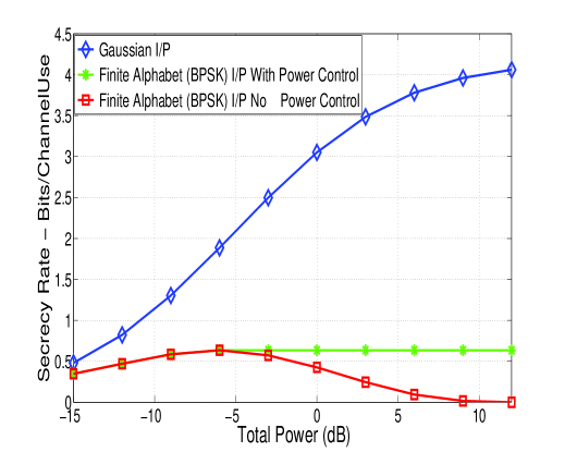
Figure 2: Secrecy rate vs total power of MIMO wiretap channel with known destination CSI and unknown (statistical) eavesdroppers CSI. $N_{S}=N_{D}=N_{E_{j}}=3,N_{0}=1,\sigma_{E_{j_{0}}}=0.5$.

VI Conclusions

We studied the problem of power allocation for secrecy in MIMO wiretap channel with finite-alphabet input. Our work differed from past works in the following aspects: we assumed that only the statistical knowledge of the eavesdropper CSI is known, and we considered multiple eavesdroppers. To study the problem, we first considered the MIMO wiretap channel with Gaussian input, where we transformed the secrecy rate max-min optimization problem to a concave maximization problem which maximized the sum secrecy rate of $l$ scalar wiretap channels subject to linear constraints on the transmit covariance matrix. When the transmit covariance matrix obtained in the Gaussian input setting is used in the finite-alphabet input setting, the secrecy rate decreased for increasing transmit powers leading to zero secrecy rate at high transmit powers. To alleviate this secrecy rate loss, we proposed a power allocation scheme using an additional power constraint in the problem. The proposed power allocation scheme was shown to alleviate the secrecy rate loss problem and achieve flat non-zero secrecy rate at high transmit powers.

In this appendix, we show that the secrecy rate with finite-alphabet input for a Gaussian wiretap channel is a unimodal function in transmit power, i.e., there exist a unique transmit power at which secrecy rate attains its maximum value. Let $y_{D}$ and $y_{E}$ be the received signals at the destination and eavesdropper, respectively, in a Gaussian wiretap channel, i.e.,

$$y_{D}=\sqrt{P}hx+\eta_{D}$$ (31)

$$y_{E}=\sqrt{P}zx+\eta_{E},$$ (32)

where $h$ and $z$ are known channel coefficients for the destination and eavesdropper channels, respectively, $x$ is the transmitted source symbol from a finite-alphabet set $\mathbb{A}$ as described in Section IV with $\mathbb{E}\{\lvert x\rvert^{2}\}=1$, $P$ is the power transmitted by the source, and $\eta_{D}$ and $\eta_{E}$ are the independent additive noise terms at the destination and eavesdropper $\sim\mathcal{CN}(0,1)$.

Using (31), the information rate at the destination, $R^{f}_{D}$, with finite-alphabet input is

$$R^{f}_{D}=I(\lvert h\rvert^{2}P).$$ (33)

Similarly, using (32), the information rate at the eavesdropper, $R^{f}_{E}$, with finite-alphabet input is

$$R^{f}_{E}=I(\lvert z\rvert^{2}P).$$ (34)

$I(.)$ in (33) and (34) is the mutual information function as defined in (24). The secrecy rate, $R^{f}_{s}$, with finite-alphabet input for the Gaussian wiretap channel is obtained as

$$R^{f}_{s}=R^{f}_{D}-R^{f}_{E}=I(\lvert h\rvert^{2}P)-I(\lvert z\rvert^{2}P).$$ (35)

With $P>0$, $R^{f}_{s}$ in (35) will be positive only when $\lvert h\rvert>\lvert z\rvert$. Therefore, w.l.o.g. we assume that $\lvert h\rvert>\lvert z\rvert$. Using Theorem 1 in [14] to find the derivatives of $R^{f}_{D}$ and $R^{f}_{E}$ w. r. t. $P$, respectively, we get

$${\frac{dR^{f}_{D}}{dP}=\lvert h\rvert^{2}\mbox{\scriptsize{MMSE}}\big{(}\lvert h\rvert^{2}P\big{)}\log_{2}{e}}$$ (36)

$${\frac{dR^{f}_{E}}{dP}=\lvert z\rvert^{2}\mbox{\scriptsize{MMSE}}\big{(}\lvert z\rvert^{2}P\big{)}\log_{2}{e}}.$$ (37)

Using (36) and (37), taking the derivative of $R^{f}_{s}$ w.r.t. $P$ and equating it to zero, we get

$${\frac{dR^{f}_{s}}{dP}=\Big{(}\lvert h\rvert^{2}\mbox{\scriptsize{MMSE}}\big{(}\lvert h\rvert^{2}P\big{)}-\lvert z\rvert^{2}\mbox{\scriptsize{MMSE}}\big{(}\lvert z\rvert^{2}P\big{)}\Big{)}\log_{2}{e}}$$

$$=0.$$ (38)

We intend to seek the solution, $P=P_{opt}$, of (38). We show that, with finite alphabet, this solution is unique and secrecy rate, $R^{f}_{s}$, attains it’s maximum value at $P=P_{opt}$.

For various $M$-ary alphabets, it is shown in [14, 15] that $1)$ MMSE is a positive, strictly monotonic decreasing function in SNR and in the limit approaches zero as SNR tends to infinity, and $2)$ at high SNRs, MMSE decreases exponentially (Theorems 3 and 4 in [14]). Since MMSE is a strictly monotonic decreasing function, it’s inverse, ${\mbox{\small{MMSE}}}^{-1}$, exists. Define

$$\alpha\ =\ \mbox{\footnotesize{MMSE}}(\lvert h\rvert^{2}P)\ \Longrightarrow\ P\ =\ \frac{1}{\lvert h\rvert^{2}}{\mbox{\footnotesize{MMSE}}}^{-1}(\alpha),$$ (39)

$$\text{and}\quad\beta\ =\ \mbox{\footnotesize{MMSE}}(\lvert z\rvert^{2}P).$$ (40)

Using (39), we rewrite (40) in terms of $\alpha$ as

$$\beta\ =\ \mbox{\footnotesize{MMSE}}(\lvert z\rvert^{2}P)\ =\ \mbox{\footnotesize{MMSE}}\Big{(}\frac{\lvert z\rvert^{2}}{\lvert h\rvert^{2}}{\mbox{\footnotesize{MMSE}}}^{-1}(\alpha)\Big{)}.$$ (41)

It can be easily shown that $\beta$ is a strictly monotonic increasing function in $\alpha$. We plot $\beta$ as a function of $\alpha$ for three different MMSE functions and two straight lines in Fig. 3. Point $(\alpha,\beta)=(0,0)\equiv O$ in the plot corresponds to $P\rightarrow\infty$. Similarly, point $(\alpha,\beta)=(1,1)$ corresponds to $P=0$.

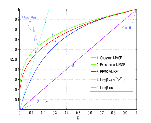
Figure 3: Various MMSE $\beta$ vs $\alpha$ curves with $\lvert h\rvert^{2}=2.0$ and $\lvert z\rvert^{2}=0.5$.

$1)\textbf{\ Gaussian MMSE Function:}$ We take $\mbox{\footnotesize{MMSE}}(\lvert h\rvert^{2}P)=\frac{1}{(1+\lvert h\rvert^{2}P)}=\alpha$ and $\mbox{\footnotesize{MMSE}}(\lvert z\rvert^{2}P)=\frac{1}{(1+\lvert z\rvert^{2}P)}=\beta$. With this choice of MMSE functions, $\beta=\frac{1}{\left(1+\frac{\lvert z\rvert^{2}}{\lvert h\rvert^{2}}({\frac{1}{\alpha}\ -\ 1})\right)}$. The slope of this curve at the origin, $(0,0)$, is

$$\frac{d\beta}{d\alpha}\ \text{at}\ (\alpha=0)\ =\ \frac{\frac{d\beta}{dP}}{\frac{d\alpha}{dP}}\ \text{as}\ (P\rightarrow\infty)\ =\ \frac{\lvert h\rvert^{2}}{\lvert z\rvert^{2}}.$$

This implies that $\beta=\big{(}\frac{\lvert h\rvert^{2}}{\lvert z\rvert^{2}}\big{)}\alpha$ is tangent to the Gaussian MMSE $\beta\ \text{vs}\ \alpha$ curve at the origin $(0,0)$.

$2)\textbf{\ Exponential MMSE Function:}$ We take $\mbox{\footnotesize{MMSE}}(\lvert h\rvert^{2}P)=\exp^{-(\lvert h\rvert^{2}P)}=\alpha$, and $\mbox{\footnotesize{MMSE}}(\lvert z\rvert^{2}P)=\exp^{-(\lvert z\rvert^{2}P)}=\beta$. With this choice of MMSE functions, $\beta={\alpha}^{(\frac{\lvert z\rvert^{2}}{\lvert h\rvert^{2}})}$. The $\beta$ axis, i.e., $\alpha=0$, is tangent to the exponential MMSE $\beta\ \text{vs}\ \alpha$ curve at the origin $(0,0)$.

$3)\textbf{\ $M$-ary MMSE Functions:}$ At high SNRs, MMSE for $M$-ary alphabets decreases exponentially (Theorems 3 and 4 in [14]). This implies that the $\beta$ axis, i.e., $\alpha=0$, is tangent to the $M$-ary MMSE $\beta\ \text{vs}\ \alpha$ curve at the origin $(0,0)$.

$4)\textbf{\ Straight Line:}$ $\beta=\big{(}\frac{\lvert h\rvert^{2}}{\lvert z\rvert^{2}}\big{)}\alpha$.

$5)\textbf{\ Straight Line:}$ $\beta=\alpha$.

Since the $\beta$ axis, i.e., $\alpha=0$, is a tangent to exponential MMSE $\beta\ \text{vs}\ \alpha$ curve at the origin $(0,0)$, the exponential MMSE $\beta\ \text{vs}\ \alpha$ curve will always intersect with the $\beta\ =\ \big{(}\frac{\lvert h\rvert^{2}}{\lvert z\rvert^{2}}\big{)}\alpha$ line at a point other than $(0,0)$. This implies that for exponential MMSE function, there exists a $P=P_{opt}$ which makes (38) zero. Uniqueness of $P_{opt}$ can be confirmed by substituting exponential MMSE function directly in (38). Also, since $\lvert h\rvert>\lvert z\rvert\geq 0$, $R^{f}_{s}$ will attain it’s maximum value at $P=P_{opt}$.

When the MMSE function is Gaussian, the Gaussian MMSE $\beta\ \text{vs}\ \alpha$ curve, $\beta=\frac{1}{\left(1+\frac{\lvert z\rvert^{2}}{\lvert h\rvert^{2}}({\frac{1}{\alpha}-1})\right)}$, does not intersect with $\beta\ =\ \big{(}\frac{\lvert h\rvert^{2}}{\lvert z\rvert^{2}}\big{)}\alpha$ line at any other point other than $(0,0)$. In fact, the $\beta=\big{(}\frac{\lvert h\rvert^{2}}{\lvert z\rvert^{2}}\big{)}\alpha$ line is tangent to the Gaussian MMSE $\beta\ \text{vs}\ \alpha$ curve at $(0,0)$. This implies that for Gaussian MMSE, there is no $P=P_{opt}$ which makes (38) zero. This fact can also be confirmed by substituting the Gaussian MMSE function directly in (38).

The MMSE function of $M$-ary alphabets at high SNRs decreases exponentially, which means $\beta$ axis, i.e., $\alpha=0$, is tangent to $M$-ary MMSE $\beta\ \text{vs}\ \alpha$ curve at the origin $(0,0)$. This implies that $M$-ary MMSE $\beta\ \text{vs}\ \alpha$ curve will always intersect with $\beta=\big{(}\frac{\lvert h\rvert^{2}}{\lvert z\rvert^{2}}\big{)}\alpha$ line at a point other than $(0,0)$. This shows that for $M$-ary MMSE function, there exists a $P=P_{opt}$ which makes (38) zero. To prove the uniqueness of $P_{opt}$, let $\lvert h\rvert^{2}\mbox{\scriptsize{MMSE}}\big{(}\lvert h\rvert^{2}P\big{)}$ and $\lvert z\rvert^{2}\mbox{\scriptsize{MMSE}}\big{(}\lvert z\rvert^{2}P\big{)}$ in (38) intersect for the first time at $P=P_{opt}$ from $P=0$. Since $\lvert h\rvert>\lvert z\rvert\geq 0$, this implies that $\lvert h\rvert^{2}\mbox{\scriptsize{MMSE}}\big{(}\lvert h\rvert^{2}P\big{)}>\lvert z\rvert^{2}\mbox{\scriptsize{MMSE}}\big{(}\lvert z\rvert^{2}P\big{)}$ for all $P<P_{opt}$ and $\lvert h\rvert^{2}\mbox{\scriptsize{MMSE}}\big{(}\lvert h\rvert^{2}P\big{)}<\lvert z\rvert^{2}\mbox{\scriptsize{MMSE}}\big{(}\lvert z\rvert^{2}P\big{)}$ in some neighborhood of $P>P_{opt}$. Monotonicity of MMSE [15] implies that $\lvert h\rvert^{2}\mbox{\scriptsize{MMSE}}\big{(}\lvert h\rvert^{2}P\big{)}$ and $\lvert z\rvert^{2}\mbox{\scriptsize{MMSE}}\big{(}\lvert z\rvert^{2}P\big{)}$ will not intersect for any finite $P>P_{opt}$. This can be seen in Fig. 4 also. This proves the uniqueness of $P_{opt}$. The above analysis also implies that at $P=P_{opt}$ the secrecy rate $R^{s}_{f}$ will attain its maximum value.

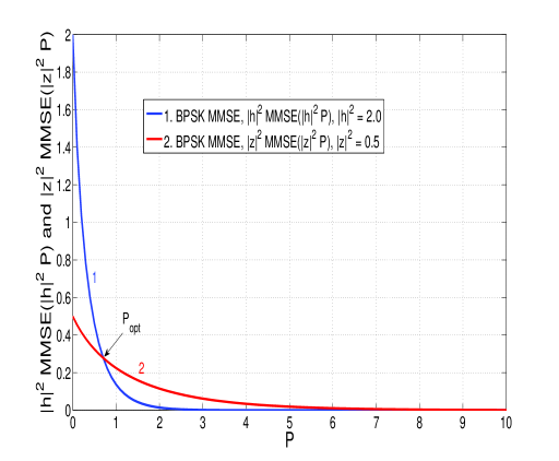
Figure 4: BPSK MMSE vs P curves with $\lvert h\rvert^{2}=2.0$ and $\lvert z\rvert^{2}=0.5$.

-A Numerical computation of $P_{opt}$

We can find $P_{opt}$ of (38) for $M$-ary MMSE functions using gradient based method as follows.

$\bf{Step\ 1:}$ Let $P_{opt}$ lie in the interval $[P_{ll},\ P_{ul}]$, $P_{ll}\geq 0$, $P_{ul}\leq P$. Let $\epsilon$ be a small positive number.

$\bf{Step\ 2:}$ $P_{opt}=(P_{ll}+P_{ul})/2$. Compute $\frac{dR^{f}_{s}}{dP}$ using (38) at $P_{opt}$.

$\bf{Step\ 3:}$ If $\frac{dR^{f}_{s}}{dP}\geq 0$, then $P_{ll}=P_{opt}$; else $P_{ul}=P_{opt}$.

Repeat $\bf{Step\ 2}$ and $\bf{Step\ 3}$ until $P_{ul}-P_{ll}\leq\delta$, where $\delta$ is a small positive number.

References

• [1] S. Shafiee and S. Ulukus, “Achievable rates in Gaussian MISO channels with secrecy constraint,” Proc. IEEE ISIT’2007, June 2007.
• [2] A. Khisti and G. Wornell, “Secure transmission with multiple antennas-I: The MISOME wiretap channel,” IEEE Trans. Inf. Theory, vol. 56, no. 7, pp. 3088-3104, July 2010.
• [3] F. Oggier and B. Hassibi, “The secrecy capacity of the MIMO wiretap channel,” Proc. IEEE ISIT’2008, July 2008.
• [4] A. Khisti and G. Wornell, “Secure transmission with multiple antennas-II: The MIMOME wiretap channel,” IEEE Trans. Inf. Theory, vol. 56, no. 7, pp. 3088-3104, July 2010.
• [5] J. Li and A. P. Petropulu, “On ergodic secrecy rate for Gaussian MISO wiretap channels,” IEEE Trans. Wireless Commun., vol. 10, no. 4, pp. 1176-1187, April 2011.
• [6] J. Liu, Y. T. Hou, and H. D. Sherali “Optimal power allocation for achieving perfect secrecy capacity in MIMO wire-tap channels,” Proc. CISS’2009, March 2009.
• [7] S. A. A. Fakoorian and A. L. Swindlehurst, “Full rank solutions for the MIMO Gaussian wiretap channel with an average power constraint,” IEEE Trans. Signal Process., vol. 61, no. 10, pp. 2620-2631, May 2013.
• [8] M. R. D. Rodrigues, A. S. Baruch, and M. Bloch, “On Gaussian wiretap channels with M-PAM inputs,” 2010 European Wireless Conference, pp.774-781, April 2010.
• [9] G. D. Raghava and B. S. Rajan, “Secrecy capacity of the Gaussian wire-tap channel with finite complex constellation input,” Online: arXiv:1010.1163v1 [cs.IT] 6 Oct 2010.
• [10] S. Bashar, Z. Ding, and C. Xiao, “On the secrecy rate of multi-antenna wiretap channel under finite-alphabet input,” IEEE Commun. Letters, vol. 15, no. 5, pp. 527-529, May 2011.
• [11] S. Vishwakarma and A. Chockalingam, “Decode-and-forward relay beamforming for secrecy with finite-alphabet input,” IEEE Commun. Letters, vol. 17, no. 5, pp. 912-915, May 2013.
• [12] Y. Wu, C. Xiao, Z. Ding, X. Gao, and S. Jin, “Linear precoding for finite-alphabet signaling over MIMOME wiretap channels,” IEEE Trans. Veh. Tech., vol. 61, no. 6, pp. 2599-2612, July 2012.
• [13] C. Paige and M. A. Saunders, “Towards a generalized singular value decomposition,” SIAM J. Numer. Anal., vol. 18, no. 3, pp. 398-405, June 1981.
• [14] A. Lozano, A. M. Tulino, and S. Verdu, “Optimum power allocation for parallel Gaussian channels with arbitrary input distributions,” IEEE Trans. Inf. Theory, vol. 52, no. 7, pp. 3033-3051, July 2006.
• [15] D. Guo, Y. Wu, S. Shamai, and S. Verdu, “Estimation in Gaussian noise: properties of the minimum mean-square error,” IEEE Trans. Inf. Theory, vol. 57, no. 4, pp. 2371-2385, April 2011.
• [16] S. Boyd and L. Vandenberghe, Convex optimization, Cambridge Univ. Press, 2004.