Holography of Wrapped M5-branes and Chern-Simons theory

Abstract

We study three-dimensional superconformal field theories on wrapped M5-branes. Applying the gauge/gravity duality and the recently proposed 3d-3d relation, we deduce quantitative predictions for the perturbative free energy of a Chern-Simons theory on hyperbolic 3-space. Remarkably, the perturbative expansion is expected to terminate at two-loops in the large $N$ limit. We check the correspondence numerically in a number of examples, and confirm the $N^{3}$ scaling with precise coefficients.

Introduction. In quantum field theories, duality refers to a map between observables of two seemingly unrelated theories. Duality can be particularly powerful when one of the two theories is not (yet) defined rigorously. There are two prominent examples in string theory: M-theory and holographic gauge/gravity duality Maldacena (1998). While less well-understood than perturbative string theory, M-theory offers a unifying framework for all string theories. The gauge/gravity duality relates a quantum field theory to a quantum gravity theory in one higher dimensions. Although the gravity theory operates mostly at the classical level, it often gives powerful predictions for the quantum field theory.

A number of new dualities have been discovered recently through compactification of M5-branes. Just as M-theory unifies string theories, M5-branes provide a unifying framework for a large class of supersymmetric quantum field theories. In the simplest case, the M5-brane theory defines a 6d conformal field theory with $(2,0)$ supersymmetry. Wrapping M5-branes on internal manifolds gives rise to lower dimensional field theories with the same or a smaller number of supersymmetries.

In conventional compactifications, the compact manifold affects the definition of the lower dimensional field theory, but does not usually bear an independent physical meaning. A novelty in recent works on M5-branes is that a duality holds between the compactified field theory and a different field theory defined on the internal manifold. For instance, in the celebrated “4d-2d” relation Gaiotto (2012); *Alday:2009aq; *Wyllard:2009hg a 4d $\mathcal{N}=2$ supersymmetric field theory is paired with an integrable field theory on a Riemann surface. Similarly, the “3d-3d” relation Terashima and Yamazaki (2011); *Terashima:2011xe; *Dimofte:2011ju; *Dimofte:2011py; *Gang:2013sqa; *Yagi:2013fda; *Lee:2013ida; *Cordova:2013cea connects a 3d $\mathcal{N}=2$ supersymmetric field theory with a 3d Chern-Simons (CS) theory.

The goal of this Letter is to point out and verify a surprising prediction for the perturbative expansion of CS theory, which is deduced from a combination of the gauge/gravity duality and the 3d-3d relation. We report on the main results here, and the details will be published elsewhere Gang et al. (2014).

We begin with wrapping a stack of $N$ M5-branes on a hyperbolic 3-manifold $M$. The resulting lower dimensional theory is called $T_{N}[M]$ Dimofte et al. (2013). One of the fundamental observables of the theory is the partition function on a squashed three-sphere, $Z_{T_{N}[M]}[S^{3}_{b}]$, with a squashing parameter $b$, and the associated free energy $F_{N,b}=-\log|Z_{T_{N}[M]}[S^{3}_{b}]|$. We will use the dualities to study properties of $F_{N,b}$ without computing it directly from $T_{N}[M]$.

On the one hand, we embed the brane configuration into the full M-theory to invoke the gauge/gravity duality. Building upon the relevant supergravity solution Gauntlett et al. (2001); *Donos:2010ax and taking the squashing into account Martelli et al. (2012), we will show that the gravity computation gives $F^{\rm gravity}=N^{3}(b+b^{-1})^{2}{\rm vol}(M)/12\pi$ in the large $N$ limit. Gauge/gravity duality leads to an equality between the gravity free energy and field theory free energy $F_{N,b}$ at large $N$. On the other hand, we use the 3d-3d relation to compute $F_{N,b}$ from the CS theory. The methods for the computation were developed recently in Dimofte (2011); Dimofte et al. (2013). A crucial feature of the 3d-3d relation is that the loop-counting parameter “$\hbar$” of the perturbative CS theory is related to the squashing parameter $b$ as $\hbar=2\pi ib^{2}$ Terashima and Yamazaki (2011); Beem et al. (2012). It follows that the $n$-th term $F^{(n)}_{N}$, defined as

$$F^{\rm CS}_{N,b}=\sum_{n=0}^{\infty}(\hbar/i)^{n-1}F_{N}^{(n)}+(\textrm{non-perturbative})\,,$$ (1)

comes from the $n$-loop diagrams of the perturbative CS theory. Comparing this asymptotic expansion with the gravity free energy, we infer: (1) $F^{(0)}_{N},F^{(1)}_{N}$ and $F^{(2)}_{N}$ all scale as $N^{3}$ and their coefficients of $N^{3}$ are proportional to ${\rm vol}(M)$. (2) Three- and higher-loop terms as well as the non-perturbative ones are suppressed at large $N$.

After reviewing the gravity computation and the methods for the CS computation, we subject our main observation to numerical tests. For a number of hyperbolic knot complements, and the value of $N$ reaching up to 30, our numerical results exhibit excellent agreement with the predictions of the dualities.

Supergravity description. It is convenient to use lower dimensional gauged supergravity for constructing various near-horizon geometries of D- or M-brane backgrounds. For M5-branes the relevant theory is 7d $SO(5)$ gauged supergravity, which is a consistent truncation of 11d supergravity. In addition to the maximally supersymmetric $AdS_{7}$, it exhibits a rich spectrum of magnetically charged $AdS$ solutions which we interpret as M5-branes wrapped on supersymmetric cycles Gauntlett et al. (2001).

In particular, we are interested in an $AdS_{4}\times M$ solution where M5-branes are wrapped on a special Lagrangian 3-cycle $M$ which is locally $H^{3}$, the hyperbolic 3-space. To implement topological twisting, one first turns on $SO(3)\subset SO(5)$ part of gauge fields so that they exactly cancel the contribution of spin connections on $H^{3}$ in the Killing spinor equation. There are also 14 scalar fields in the traceless symmetric tensor representation of $SO(5)$, and we turn on a single scalar field which is singlet under the remaining symmetry $SO(3)\times SO(2)$.

It turns out that the supersymmetry and the equation of motion uniquely determine the $AdS_{4}\times H^{3}$ solution Gauntlett et al. (2001). One can then use the uplifting formula to obtain a solution of 11d supergravity. The metric is

$${\rm d}s^{2}_{11}=\frac{2^{2/3}(1+\sin^{2}\theta)^{1/3}}{g^{2}}\Bigg{[}{\rm d}s^{2}(AdS_{4})+{\rm d}s^{2}(M)$$

$$\qquad+\frac{1}{2}\left(d\theta^{2}+\frac{\sin^{2}\theta}{1+\sin^{2}\theta}d\phi^{2}\right)+\frac{\cos^{2}\theta}{1+\sin^{2}\theta}d\tilde{\Omega}_{2}\Bigg{]},$$ (2)

where $0<\theta<\pi/2,0<\phi<2\pi$. $M$ is locally $H^{3}$. Both $AdS_{4}$ and $M$ have unit radius. ${\rm d}\tilde{\Omega}_{2}$ denotes the unit 2-sphere, twisted by the spin connection one-forms of $M$.

The parameter $g$ is the coupling constant of 7d supergravity, and sets the overall curvature scale of the solution. Through the flux quantization, $g$ is related to the number of M5-branes $N$. The 4-form field $G$ of 11d supergravity, when restricted to the internal space $X_{4}$, is

$$G|_{X_{4}}=-\frac{1}{g^{3}}{\rm d}\left[\frac{\cos^{3}\theta}{1+\sin^{2}\theta}\right]\wedge{\rm d}\phi\wedge{\rm vol}(\tilde{S}^{2})\,.$$ (3)

Integrating this, one obtains $N=(\pi l_{\rm P}^{3}g^{3})^{-1}$, where $l_{\rm P}$ is 11d Planck length.

The gravity side computation of the partition function can be done using the standard AdS/CFT prescription. That is, we calculate the holographically renormalized on-shell action for the supergravity solution. For round $S^{3}$, the result is simply $F=\frac{\pi}{2G_{4}}$, where $G_{4}$ is 4d Newton’s constant. See e.g. Emparan et al. (1999); *Gabella:2011sg for derivation.

To invoke the 3d-3d relation we put the wrapped M5-brane theory on an ellipsoid $S^{3}_{b}$, defined by $b^{2}(x_{1}^{2}+x_{2}^{2})+b^{-2}(x_{3}^{2}+x_{4}^{2})=1$. The geometry has a manifest $b\leftrightarrow b^{-1}$ symmetry and so do all partition functions in this Letter. For the holographic computation on $S^{3}_{b}$, we consider the minimal ${\cal N}=2$ gauged supergravity in 4d, and look for a particular supersymmetric solution whose metric and the Killing spinors reproduce the $S^{3}_{b}$ metric and its Killing spinor given in Hama et al. (2011), as one approaches the boundary. Such a solution is presented in Martelli et al. (2012), which is a class of Plebanski-Demianski solutions in Einstein-Maxwell theory. Then the 11d solution (2) should change accordingly, as one plugs the solution in Martelli et al. (2012) into the uplifting formula of Gauntlett et al. (2001). But it is also established in Martelli et al. (2012) that the $b$-dependence of the holographic free energy is universally given as $F_{b}=(b+1/b)^{2}F_{b=1}/4$. One may thus first compute $F_{b=1}$ using (2) and restore $b$-dependence easily.

$$F^{\rm gravity}=\frac{N^{3}}{12\pi}\left(b+\frac{1}{b}\right)^{2}\textrm{vol}(M)\,.$$ (4)

This is the key result we check against the field theory in this Letter. Since the gravity analysis is classical, $F^{\rm gravity}$ captures only the leading $N^{3}$ term at large $N$. On the other hand, its $b$-dependence is exact as coefficient of $N^{3}$. For knot complements $M=S^{3}\backslash K$, the solution (2) needs to be modified to incorporate intersecting M5-branes along the knot. For 4d theories of class $S$ associated with a Riemann surface $\Sigma_{g,h}$ of genus $g$ with $h$ full punctures, the leading $N^{3}$ terms of conformal anomaly coefficients $a$ and $c$ depend only on the Euler characteristic of the Riemann surface regardless of the existence of punctures Gaiotto and Maldacena (2012). In a similar vein, as the hyperbolic volume is a topological invariant, we expect the formula (4) to be robust and insensitive to the presence of the knot $K$.

3d-3d relation and a $PGL(N)$ CS theory. The 3d-3d relation Terashima and Yamazaki (2011); Dimofte et al. (2011); Cordova and Jafferis (2013) states a precise map between $T_{N}[M]$ and the analytically continued $PGL(N)$ CS theory on $M$. The map for supersymmetric partition function is

$$Z_{T_{N}[M]}[S^{3}_{b}]=Z^{\rm CS}_{N}[M;\hbar]\;.$$ (5)

In this Letter, we focus on the case when the 3-manifolds are hyperbolic knot complements on $S^{3}$, $M=S^{3}\backslash K$, obtained by removing a tubular neighborhood of a hyperbolic knot $K$ from $S^{3}$. A unique complete hyperbolic metric is known to exist for each $M=S^{3}\backslash K$. For the notation of knots we follow Rolfsen (1976). The volume of $M$ can be expressed in terms of dilogarithm, e.g. $\textrm{vol}(S^{3}\backslash{\bf 4}_{1})=2\textrm{Im}\big{(}{\rm Li}_{2}(e^{\frac{i\pi}{3}})\big{)}=2.02988\cdots$.

A knot complement $M$ has a torus boundary and $T_{N}[M]$ has a flavor symmetry of rank $N-1$ which will be enhanced to $SU(N)$ at IR Dimofte et al. (2013). Both sides of (5) are functions of complex parameters $\{\mu_{i}\}_{i=1}^{N-1}$. For $T_{N}[M]$, $\mu_{i}$ are complexified mass parameters

$$\mu_{i}=2\pi b\left(m_{i}+\frac{i}{2}(b+b^{-1})r_{i}\right)\;,$$ (6)

where $m_{i}$ and $r_{i}$ are real masses and R-charges coupled to the $U(1)^{N-1}$ flavor symmetry. For comparison with $AdS_{4}$ gravity, the conformal symmetry requires $m_{i}=0$ and $r_{i}$ are determined via maximization of the free energy on $S^{3}$ Jafferis (2012). The symmetry enhancement to $SU(N)$ leads to $r_{i}=0$ which are invariant under Weyl reflections. For the CS theory, we consider a boundary condition which fixes the conjugacy class of gauge holonomy along the meridian cycle of $\partial M$. $\mu_{i}$ parametrizes the meridian holonomy.

The action for the CS theory is

$$S_{\rm CS}[{\cal A},\bar{{\cal A}}]=\frac{i}{2\hbar}CS[\mathcal{A}]+\frac{i}{2\tilde{\hbar}}CS[\bar{\mathcal{A}}]\;,$$ (7)

$$CS[\mathcal{A}]:=\int_{M}\textrm{Tr}({\cal A}\wedge d{\cal A}+\frac{2}{3}{\cal A}\wedge{\cal A}\wedge{\cal A})\;.$$ (8)

We consider an analytic continuation of the theory Witten (2010) where $\hbar,\tilde{\hbar}$ are complex and ${\cal A},\bar{{\cal A}}$ are independent gauge fields. $\hbar$ and $\tilde{\hbar}$ are mapped through the 3d-3d relation to the squashing parameter $b$ as Terashima and Yamazaki (2011); Beem et al. (2012)

$$\hbar=2\pi ib^{2}\;,\quad\tilde{\hbar}=-4\pi^{2}/\hbar=2\pi ib^{-2}\;.$$ (9)

Formally, $Z_{N}^{\rm CS}[M]$ can be written as a path-integral,

$$Z_{N}^{\rm CS}[M](\mu_{i})=\int D{\cal A}D\bar{{\cal A}}|_{\rm b.c.}e^{iS_{\rm CS}[{\cal A},\bar{\cal A}]}\;,$$ (10)

with the boundary condition $|_{\rm b.c.}$ specified by $\{\mu_{i}\}$. In practice, it is more convenient to use canonical quantization. The classical solutions are flat-connections,

$$\mathcal{F}=d{\cal A}+{\cal A}\wedge{\cal A}=0\;,\quad\bar{\mathcal{F}}=d{\bar{\cal A}}+{\bar{\cal A}}\wedge{\bar{\cal A}}=0\;.$$ (11)

For quantization, we first consider a classical phase space ${\mathcal{P}(\partial M)}$ associated with the boundary of $M$,

$$\mathcal{P}_{N}(\partial M)=\{\mathcal{A},\bar{\mathcal{A}}|\mathcal{F}=\bar{\mathcal{F}}=0\textrm{ on $\partial M$}\}/\mbox{(gauge)}\;,$$

and its Lagrangian submanifold associated with $M$ Dimofte et al. (2009),

$$\mathcal{L}_{N}(M)=\{\mathcal{A},\bar{\mathcal{A}}|\mathcal{F}=\bar{\mathcal{F}}=0\textrm{ on $M$}\}/\mbox{(gauge)}\;.$$

After quantization, the phase space is replaced by a Hilbert-space $\mathcal{H}_{N}(\partial M)$, and $\mathcal{L}_{N}(M)$ by a state $|M_{N}\rangle\in\mathcal{H}_{N}(\partial M)$. The dimension of the phase space is $2(N-1)$ and we choose the meridian $\{\mu_{i}\}$ as position variables. Collecting all the ingredients, the CS partition function (10) can be identified as a wave-function Dimofte et al. (2009),

$$Z^{\rm CS}_{N}[M](\mu_{i})=\langle\mu_{i}|M_{N}\rangle\;.$$ (12)

It is possible to write down an integral expression for $Z_{N}^{\rm CS}$, thanks to the two recently developed tools: $N$-decomposition of $M$ Dimofte et al. (2013) and a state-integral model in Dimofte (2011). They both make use of an ideal triangulation of $M$,

$$M=\left(\bigcup_{i=1}^{k}\Delta_{i}\right)/(\textrm{gluing data})\;.$$ (13)

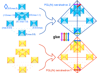
Figure 1: $N$-decomposition for $M=S^{3}\backslash\mathbf{4}_{1}$. $M$ is decomposed into two tetrahedra $Y$ and $Z$. Each tetrahedron is decomposed into a pyramid of $\tfrac{1}{6}N(N^{2}-1)$ octahedra.

Dividing each $\Delta_{i}$ further into a pyramid of $N(N^{2}-1)/6$ octahedra ($\Diamond$), we obtain a $N$-decomposition of $M$,

$$M=\left(\bigcup_{i=1}^{k}\bigcup_{(a,b,c,d)}\Diamond^{(i)}_{(a,b,c,d)}\right)/(\textrm{gluing data})\;.$$ (14)

The gluing data dictate how we should match the vertices from different octahedra. The octahedra in each $\Delta_{i}$ are labelled by four non-negative integers $(a,b,c,d)$ whose sum is $N-2$. The decomposition is a mathematical tool to construct the moduli spaces ${\cal P}(\partial M)$ and ${\cal L}(M)$ by ‘gluing’ the building blocks ${\cal P}(\partial\Diamond)$ and ${\cal L}(\Diamond)$ .

The state-integral model Dimofte (2011); Dimofte and Garoufalidis (2012) is obtained by quantizing the gluing procedure of constructing flat connection moduli spaces. The model provides a finite dimensional integral expression for $Z^{\rm CS}_{N}[M]$. At conformal point $\mu_{i}=0$, ($\mathcal{M}_{N}:=\frac{k}{6}N(N^{2}-1)$)

$$Z^{\rm CS}_{N}[M]=\frac{1}{\sqrt{\det B_{N}}}\int\frac{d^{\mathcal{M}_{N}}X}{(2\pi\hbar)^{\mathcal{M}_{N}/2}}\prod\psi_{\hbar}(X)\times$$

$$\exp\left[-\frac{1}{\hbar}(i\pi+\frac{\hbar}{2})X^{T}B_{N}^{-1}\nu_{N}+\frac{1}{2\hbar}X^{T}B_{N}^{-1}A_{N}X\right],$$ (15)

up to prefactors independent of $N$ and an overall phase factor. $\psi_{\hbar}(X)$ is a non-compact quantum dilogarithm function, which is roughly $Z^{\rm CS}_{2}[\Diamond]$ Dimofte (2011). $\{A_{N},B_{N}\}$ are $\mathcal{M}_{N}\times\mathcal{M}_{N}$ matrices and $\nu_{N}$ is an $\mathcal{M}_{N}$-dimensional column vector with integer entries. They can be determined from the gluing data of the $N$-decomposition up to a certain ambiguity which does not affect our discussion.

Perturbative CS theory vs gravity. In the limit $\hbar\rightarrow 0$, $Z^{\rm CS}_{N}[M]$ can be evaluated perturbatively using the saddle point approximation leading to an expansion of the form (1). The perturbative “invariants” $F_{N}^{(n)}$ can be systematically computed using the Feynman rules derived in Dimofte and Garoufalidis (2012). Remarkably enough, in view of the dictionary (9), we find the gravity free energy (4) displays the same expansion structure as the CS counterpart but terminates at two-loop. Combining $F^{\rm gravity}=F^{\rm gauge}$ with the 3d-3d relations (5) and (9), we conclude

$$\lim_{N\rightarrow\infty}\frac{F_{N}^{(n)}}{N^{3}}=c_{n}\textrm{vol}(M)\;,$$ (16)

with $c_{0}=\frac{1}{6},c_{1}=\frac{1}{6\pi},c_{2}=\frac{1}{24\pi^{2}}$ and $c_{n}=0$ for $n\geq 3$. If the predictions are correct, the symmetry $b\leftrightarrow b^{-1}$ exists even in the perturbative expansion at large $N$, which gives a strong evidence that non-perturbative corrections in (1) will be suppressed in the limit. The prediction on the classical part $F^{(0)}$ can be understood intuitively Dimofte et al. (2013). First, we recall that ${\rm Im}(CS[{\cal A}])$ for $PGL(2)$ is equivalent to the 3d $AdS$ gravity action Witten (1988). The unique complete hyperbolic metric on $M$ is mapped to a geometrical flat connection ${\cal A}^{(\rm geom)}_{N=2}$. The flat $PGL(2)$-connection can be lifted to a flat $PGL(N)$-connection ${\cal A}_{N}^{({\rm geom})}$ using the irreducible $N$-dimensional representation of $PGL(2)$. We assume that conjugate $\overline{{\cal A}_{N}^{({\rm geom})}}$ of the $PGL(N)$ gives a dominant contribution to the path-integral (10) when $\mu_{i}=0$. Elementary algebra gives

$$CS[\overline{{\cal A}^{({\rm geom})}_{N}}]=\frac{1}{6}N(N^{2}-1)CS[\overline{{\cal A}^{({\rm geom})}_{2}}]\;.$$ (17)

Combining this with the fact that $F_{2}^{(0)}={\rm Im}(CS)/2$ for $\overline{{\cal A}^{(\rm geom)}_{N=2}}$ equals to $\textrm{vol}(M)$, we arrive at (16) for $n=0$. The prediction on $F^{(1)}_{N}$ can be proved using results in Menal-Ferrer and Porti (2011). A perturbative analysis of the CS theory gives $F^{(1)}_{N}=-\frac{1}{2}\log|\textrm{Tor}_{\textbf{adj}}[M,\overline{\mathcal{A}^{\textrm{(geom)}}_{N}}]|$ where $\textrm{Tor}_{\rho}[M,\mathcal{A}]$ is the Ray-Singer torsion of an associated vector bundle in a representation $\rho$ twisted by a flat connection $\mathcal{A}$. In Menal-Ferrer and Porti (2011), it is proven that

$$\lim_{m\rightarrow\infty}\frac{1}{m^{2}}\log\textrm{Tor}_{\rho_{m}}[M,\mathcal{A}^{(geom)}_{N=2}]=-\frac{1}{4\pi}\textrm{vol}(M)\;,$$ (18)

where $\rho_{m}$ is the irreducible $m$-dimensional representation of $PGL(2)$. Applying the theorem to $F^{(1)}_{N}$ using the branching rule $\textbf{adj}=\rho_{3}\oplus\rho_{5}\oplus\ldots\oplus\rho_{2N-1}$, we arrive at (16) for $n=1$.

We currently have little analytic understanding of the loop invariants $F_{N}^{(n)}$ $(n\geq 2)$. In particular, the appearance of ${\rm vol}(M)$ in the 2-loop term is striking and seems non-trivial to prove.

We have verified (16) for several examples of $M$ by calculating the invariants $F_{N}^{(1)}$, $F_{N}^{(2)}$ and $F_{N}^{(3)}$ numerically as we vary $N$. The computation of the gluing data $\{A_{N},B_{N},\nu_{N}\}$ is greatly facilitated by the computer package SnapPy Culler et al. ; Garoufalidis et al. (2012). Our results are summarized in Fig. 2, which shows log-log plots of $F^{(1)}$ and $F^{(2)}$. They clearly exhibit the expected $N^{3}$ behavior already at modest values of $N\sim 10$.

Figure 2: Log-log plot of $F_{N}^{(1)}$ (Left) and $F_{N}^{(2)}$(Right) vs. $N$, for $N=6,\cdots,N_{\rm max}$ for the seven simplest hyperbolic knot complements $M=S^{3}\backslash K$ ($K={\bf 4}_{1},{\bf 5}_{2},{\bf 6}_{1},{\bf 6}_{2},{\bf 6}_{3},{\bf 7}_{2},{\bf 7}_{3}$). $N_{\rm max}$ for each $M$ is limited by computing time.

To extract the coefficient of $N^{3}$ term efficiently, we computed the third-differences $F_{N}^{(1)}{}^{\prime\prime\prime}$ and $F_{N}^{(2)}{}^{\prime\prime\prime}$ and confirmed that they quickly converge to the exact values of ${\rm vol}(M)$ up to overall factors $\frac{1}{\pi}$ and $\frac{1}{4\pi^{2}}$ respectively, as we increase $N$. The results summarized in the table below show excellent agreement.

$K$	vol($S^{3}\backslash K$)	$\pi F_{N}^{(1)}{}^{\prime\prime\prime}$	$(N)$	$4\pi^{2}F_{N}^{(2)}{}^{\prime\prime\prime}$	$(N)$
$\mathbf{4}_{1}$	2.02988	2.03001	($27$)	2.02898	($17$)
$\mathbf{5}_{2}$	2.82812	2.82828	($12$)	2.82674	($12$)
$\mathbf{6}_{1}$	3.16396	3.20648	($12$)	3.15574	($12$)
$\mathbf{6}_{2}$	4.40083	4.40364	($12$)	4.39929	($12$)
$\mathbf{6}_{3}$	5.69302	5.69464	($11$)	5.68799	($9$)
$\mathbf{7}_{2}$	3.33174	3.56613	($12$)	3.27455	($12$)
$\mathbf{7}_{3}$	4.59213	4.58680	($12$)	4.58331	($11$)

The computation of 3-loop invariant $F_{N}^{(3)}$ takes significantly longer, due to the large number of Feynman diagrams. We have done the computation for $\mathbf{4}_{1}$ and obtained $F_{N}^{(3)}=0.03128,0.02844,0.02602$ for $N=7,8,9$. It is thus strongly suggested that $\lim_{N\rightarrow\infty}F_{N}^{(3)}/N^{3}=0$, in accordance with the holographic prediction.

Discussion. In this Letter we have performed a quantitive study of $AdS_{4}/CFT_{3}$ arising from wrapped M5-branes, by comparing the free energy on both sides. We confirm the famous $N^{3}$-behavior of the M5-brane physics including an overall factor. It is highly desirable to have an analytic proof of the predictions on the perturbative $PGL(N)$ CS invariants on hyperbolic 3-manifolds in the large $N$ limit. Studying other physical objects, such as defects, will certainly give new insights and deserve further exploration.

Acknowledgments. We are grateful to J. P. Gauntlett and M. Yamazaki for invaluable comments on the manuscript. This work was supported by NRF grants funded by the Korea government with grant No. 2010-0023121, 2012046278 (NK) and 2012R1A1B3001085, 2012R1A2A2A02046739 (SL).

References

- Maldacena (1998) J. M. Maldacena, Adv.Theor.Math.Phys., 2, 231 (1998), arXiv:hep-th/9711200 [hep-th] .
- Gaiotto (2012) D. Gaiotto, JHEP, 1208, 034 (2012), arXiv:0904.2715 [hep-th] .
- Alday et al. (2010) L. F. Alday, D. Gaiotto, and Y. Tachikawa, Lett.Math.Phys., 91, 167 (2010), arXiv:0906.3219 [hep-th] .
- Wyllard (2009) N. Wyllard, JHEP, 0911, 002 (2009), arXiv:0907.2189 [hep-th] .
- Terashima and Yamazaki (2011) Y. Terashima and M. Yamazaki, JHEP, 1108, 135 (2011), arXiv:1103.5748 [hep-th] .
- Terashima and Yamazaki (2013) Y. Terashima and M. Yamazaki, Phys.Rev., D88, 026011 (2013), arXiv:1106.3066 [hep-th] .
- Dimofte et al. (2011) T. Dimofte, D. Gaiotto, and S. Gukov, (2011a), arXiv:1108.4389 [hep-th] .
- Dimofte et al. (2011) T. Dimofte, D. Gaiotto, and S. Gukov, (2011b), arXiv:1112.5179 [hep-th] .
- Gang et al. (2013) D. Gang, E. Koh, S. Lee, and J. Park, (2013), arXiv:1305.0937 [hep-th] .
- Yagi (2013) J. Yagi, JHEP, 1308, 017 (2013), arXiv:1305.0291 [hep-th] .
- Lee and Yamazaki (2013) S. Lee and M. Yamazaki, (2013), arXiv:1305.2429 [hep-th] .
- Cordova and Jafferis (2013) C. Cordova and D. L. Jafferis, (2013), arXiv:1305.2891 [hep-th] .
- Gang et al. (2014) D. Gang, N. Kim, and S. Lee, to appear (2014).
- Dimofte et al. (2013) T. Dimofte, M. Gabella, and A. B. Goncharov, (2013), arXiv:1301.0192 [hep-th] .
- Gauntlett et al. (2001) J. P. Gauntlett, N. Kim, and D. Waldram, Phys.Rev., D63, 126001 (2001), arXiv:hep-th/0012195 [hep-th] .
- Donos et al. (2010) A. Donos, J. P. Gauntlett, N. Kim, and O. Varela, JHEP, 1012, 003 (2010), arXiv:1009.3805 [hep-th] .
- Martelli et al. (2012) D. Martelli, A. Passias, and J. Sparks, Nucl.Phys., B864, 840 (2012), arXiv:1110.6400 [hep-th] .
- Dimofte (2011) T. Dimofte, (2011), arXiv:1102.4847 [hep-th] .
- Beem et al. (2012) C. Beem, T. Dimofte, and S. Pasquetti, (2012), arXiv:1211.1986 [hep-th] .
- Emparan et al. (1999) R. Emparan, C. V. Johnson, and R. C. Myers, Phys.Rev., D60, 104001 (1999), arXiv:hep-th/9903238 [hep-th] .
- Gabella et al. (2011) M. Gabella, D. Martelli, A. Passias, and J. Sparks, JHEP, 1110, 039 (2011), arXiv:1107.5035 [hep-th] .
- Hama et al. (2011) N. Hama, K. Hosomichi, and S. Lee, JHEP, 1105, 014 (2011), arXiv:1102.4716 [hep-th] .
- Gaiotto and Maldacena (2012) D. Gaiotto and J. Maldacena, JHEP, 1210, 189 (2012), arXiv:0904.4466 [hep-th] .
- Rolfsen (1976) D. Rolfsen, Knots and Links (Publish or Perish, Berkeley, 1976).
- Jafferis (2012) D. L. Jafferis, JHEP, 1205, 159 (2012), arXiv:1012.3210 [hep-th] .
- Witten (2010) E. Witten, (2010), arXiv:1001.2933 [hep-th] .
- Dimofte et al. (2009) T. Dimofte, S. Gukov, J. Lenells, and D. Zagier, Commun.Num.Theor.Phys., 3, 363 (2009), arXiv:0903.2472 [hep-th] .
- Dimofte and Garoufalidis (2012) T. D. Dimofte and S. Garoufalidis, ArXiv e-prints (2012), arXiv:1202.6268 [math.GT] .
- Witten (1988) E. Witten, Nucl.Phys., B311, 46 (1988).
- Menal-Ferrer and Porti (2011) P. Menal-Ferrer and J. Porti, ArXiv e-prints (2011), arXiv:1110.3718 [math.GT] .
- (31) M. Culler, N. Dunfield, and J. R. Weeks, SnapPy http://snappy.computop.org.
- Garoufalidis et al. (2012) S. Garoufalidis, M. Goerner, and C. K. Zickert, ArXiv e-prints (2012), arXiv:1207.6711 [math.GT] .