Communities of dense weighted networks: MicroRNA co-target network as an example

Abstract

Complex networks are intrinsically modular. Resolving small modules is particularly difficult when the network is densely connected; wide variation of link weights invites additional complexities. In this article we present an algorithm to detect community structure in densely connected weighted networks. First, modularity of the network is calculated by erasing the links having weights smaller than a cutoff $q.$ Then one takes all the disjoint components obtained at $q=q_{c},$ where the modularity is maximum, and modularize the components individually using Newman Girvan’s algorithm for weighted networks. We show, taking microRNA (miRNA) co-target network of Homo sapiens as an example, that this algorithm could reveal miRNA modules which are known to be relevant in biological context.

Keywords : modularization algorithm, microRNA co-target network, community structure

1 Introduction

Networks, a set of nodes or vertices joined pairwise by links or edges, are commonly used for describing sociological (scientific collaborations [1] and acquaintance networks [2]), biological (proteins interactions, genes regulatory, food webs, neural networks, metabolic networks), technological (Internet and the web) and communication (airport [3], road [4, 5], and railway network [6, 7]) systems. The topological properties of these complex networks [8, 9] help in identifying underlying community structures [10], network motifs [11], connectivity [12, 13] and several other properties [14]. The links of a network can also be weighted. Some of the networks are associated with links of varying strengths [15, 16, 17] represented by link weights. The topological properties of weighted networks [18, 19] are quite different and their study requires additional care. In particular when link weights vary in a wide range, one need to identify suitably the irrelevant links and ignore them to simplify the network [20].

Most networks in nature, whether weighted or not, exhibit community (or modular) structures. Detection of communities in the complex networks provide invaluable information on the underlying synergism. Nodes which belong to a particular module are more than likely to function together for some common cause; being able to unravel such communities help in identifying functional properties of the network. For example in social networks [21], communities observed are based on interests, age, profession of the people. Similarly, communities reflects the themes of the web-pages in World Wide Web, related papers on a single topic in citation networks [22], subsystems within ecosystems [23, 24] in food webs, and it may relate to functional groups [25, 26] in cellular and metabolic networks.

To identify the modular structures of complex networks, several algorithms [27, 28, 29, 30] are developed recently. But most of these methods are context based and a unique algorithm which could work universally is still out of reach. Recently Newman and Girvan has proposed a couple of methods [10, 31, 32] to detect the modules but they take high computational time for large networks. Later, a faster algorithm [33] is being put forward by the same authors, based on maximization of modularity $M$ defined as the number of edges present within the groups minus the expected number in an equivalent random network. According to this algorithm, best partition of a network is the one which has maximum modularity $M.$ This modularization method [33] is further generalized to include weighted networks [34].

Newman Girvan’s modularization algorithms (NGM), though widely used for finding modules of both weighted and unweighted networks, has some shortcomings [35]. It was argued that modularity maximization algorithm can resolve the network upto a scale that depends on the total number of links $l;$ a module having more than $\sqrt{l/2}$ links can not be resolved even when it is a clique and connected to external modules through just one link. Moreover the situation gets worse when substantial number of small communities coexist with large ones. This observation is also true for weighted networks [36]. Therefore modularity maximization uncovers only large modules missing important substructures which are small. In this context, an clustering method has been proposed recently by Mookherjee et. al. [20] in context of microRNA co-target network of human which is densely connected by weighted links. The authors claimed to obtain microRNA clusters which reveal biologically significant processes and pathways. This algorithm also suffers from certain short comings. First, the method has in-built arbitrariness in determining the total number of clusters and then its sub-structures connected by large-weighted links, if any, remains undetectable. Details of the algorithm and its shortcomings are discussed in the next section.

In this article we propose a new algorithm in an effort to overcome these shortcomings and to efficiently determine the communities of any dense weighted network. We demonstrate the algorithm using the microRNA co-target network of Homo sapiens and compare the modules with those obtained by NGM algorithm for weighted networks [34] and the clustering algorithm [20].

2 Clustering algorithm

In a recent article [20], Mookherjee et. al. have proposed an algorithm to find clusters of miRNA co-target network of Homo sapiens. MicroRNAs are short non-coding RNAs which usually suppress gene expression in post-transcriptional level [37]. Taking the predicted targets of $711$ miRNAs of Homo sapiens from Microcosm Target database [38], the authors constructed the co-target network by joining miRNAs pairwise by weighted links. The link weight $w$ corresponds to the number of common targets of the concerned pair. The network thus constructed consists of $711$ miRNAs (nodes) and $252405$ edges. Since the network is fully connected, it is evident that clusters containing less than half the number of nodes can not be resolved by standard algorithms [31, 34]. To obtain the clusters of this densely packed network Mookherjee et. al. in [20] have adopted the following strategy.

The link weights of this network vary in a wide range: minimum being $1$ and maximum $1253.$ Thus most links are considered irrelevant in determining the clusters. In an attempt to simplify the network, links with weights smaller than a pre-defined cutoff value $q$ are erased; the resulting network breaks into small disjoint components. Denoting, $N(q)$ as the number components the authors find that $N(q)$ does not increase substantially until $q$ reaches a threshold value $q^{*}$ and then it breaks quickly into large number of components (Fig. 2C in [20]). Thus the network is optimally connected at $q^{*}=103$ where ${d\over dq}N(q)$ is maximum. Among all the components obtained at $q^{*}=103,$ the largest one ${\cal G}$ contains $479$ miRNAs. A large fraction of miRNAs present in ${\cal G}$ are found to down regulate expression of genes involved in several genetic diseases. To explore how miRNAs are organized in ${\cal G},$ $q$ is increased further until the total number of components does not change much. At $q=160,$ the subgraph ${\cal G}$ has $70$ components (called miRNA clusters) and $149$ lone miRNAs. Note that if we consider all $711$ miRNAs, instead of $479$ miRNAs belonging to ${\cal G},$ the total number of clusters would have been $94$ (see Table 3 for details).

Further, the authors have analyzed these $70$ clusters and claimed that they are biologically relevant -either pathway or tissue or disease specific. Note that, even though the targets are predicted based on sequence similarities, the microRNA clusters reveals functionality quite well; only about $11$ clusters are found to contain miRNAs of identical seed sequence. Thus it is suggestive that a group of miRNA, instead of individual ones, are involved in carrying out necessary functions.

Limitations : Although the cluster finding algorithm discussed in [20] partitions the miRNA co-target network into several components which provide significant information about the functions of miRNA clusters, it suffers from certain limitations. Firstly, there exists few clusters containing a large number (as large as $47$) of miRNAs; such large clusters produce significant noise in identifying pathways and functions from enhancement analysis.

Figure 1: The above network consists of two distinct modules (A and B) connected by only two links.

Secondly, if a miRNA cluster has two or more sub-structures which are connected by a few links having weights much larger than $q^{*},$ it is beyond the scope of this algorithm to resolve them. For example the network in Fig. 1 clearly has two modules but weight of the few links that joins the two modules are larger than $q^{*}.$ Since the algorithm looks for disconnected components of the graph, it is not possible to uncover these two obvious modules (A and B). Lastly to reveal the sub-structures of a giant cluster ${\cal G},$ $q$ is increase to an arbitrary value (taken as $160$ in [20]). In practice the actual number of clusters depends weakly on this choice, however it still introduces an arbitrariness in the algorithm. All these shortcomings necessitates exploring other appropriate algorithms for finding the community structure in dense weighted network.

3 The proposed algorithm

In this section we proposed an algorithm for finding modules of dense weighted networks. The algorithm primarily consists of two steps -first, finding the major communities and second, extracting their sub-structures.

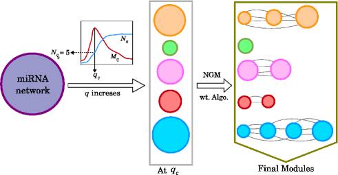
Figure 2: The outline of our algorithm that has been developed to find the modules of the densely linked weighted network.

Step I: For finding the modular structures, we consider a weighted network which is densely connected. Let the network has $M$ nodes denoted by $i=1,2,\dots M$ and a connected pair of nodes $i$ and $j$ has non zero weight $W_{ij}.$ Thus, the network is represented by an adjacency matrix $W$ with elements

$$W_{ij}=\left\{\begin{array}[]{cc}w&{\rm if}~{}~{}i~{}~{}{\rm and}~{}~{}j~{}~{}{\rm are~{}~{}connected}\cr 0&{\rm otherwise}\end{array}\right..$$ (1)

We also assume that the network is densely connected. A preliminary simplification can be done following Ref. [20], where links with weights smaller than a pre-decided cutoff $q$ are erased. The resulting network thus breaks up into smaller disconnected components -say $N(q)$ in total. It is evident that $N(q)$ is the number of diagonal blocks of a matrix $W^{q}$ with elements

$$W_{ij}^{q}=\left\{\begin{array}[]{cc}0&\textrm{if~{}}W_{ij}<q\cr W_{ij}&\rm{otherwise}\end{array}\right..$$

Clearly $N(q)$ must strictly be a non-decreasing function with $N(q=0)=1.$

We proceed further to calculate the modularity of the concerned weighted network for different values of $q.$ In general, if a network (weighted) has $c$ partitions, one can calculate the modularity [34] from knowing the set of nodes which belong to each partition,

$$M={1\over 2m}\sum_{l=1}^{c}\sum_{ij}\left(W_{ij}-{k_{i}k_{j}\over 2m}\right)S_{ij}^{l}$$ (2)

where $k_{i}=\sum_{j}W_{ij}$ represents sum of the weights of the edges attached to node $i$ and $m=\sum_{i}k_{i}.$ The term $S_{ij}^{l}$ is $1$ only if vertices $i$ and $j$ belong to same group. For a given $q,$ we take the components as the modules (thus $c=N(q)$) and denote corresponding modularity as $M(q).$ Note that, unlike $N(q),$ the modularity $M(q)$ need not be a increasing function. A schematic plot of these functions are shown in Fig. 2. Since, large modularity is a feature of better community structure we choose the value $q_{c}$ where $M(q)$ takes the maximum value and then collect set of components obtained there for further analysis.

Step II : The number of miRNAs present in each of the components, $i.e.,$ the component sizes obtained at $q_{c},$ are quite large. To get finner division of these components we can increase the $q$ value further, then although we will get smaller sized groups but the value of $M(q)$ will decrease, which is not favorable. So keeping the value of $q$ fixed at $q_{c}$ where $M(q)$ is maximum, we find the further groups present in these individual components by using NGM algorithm for weighted networks [34]. Taking the components one by one we then find their modules with help of NGM algorithm for weighted network [34], and accept the partition if the modularity value for this partition is positive or other wise we ignore it. Likewise we consider each of the components formed at $q_{c}$ for further partitioning. Collection of all the partitioned components of the network are then considered as the final modules of the weighted network.

4 Example case study

We demonstrate this algorithm for miRNA co-target network of human, a dense and weighted network constructed and studied by Mookherjee $et.al.$ [20]. MicroRNAs (miRNAs) are small single stranded $\sim 22$nt long non-coding RNAs [39] that repress gene expression by binding $3^{\prime}$-untranslated regions ($3^{\prime}$ UTR) of messenger RNA (mRNA) target transcripts, causing translational repression [37]. Being a secondary regulator, miRNAs usually repress the gene expression marginally. Thus it is natural to expect that cooperative action of miRNAs are needed for alteration of any biological function or pathway. MicroRNA synergism has been a recent focus in biology for studying their regulatory effects in cell. Recent articles [20, 40] have identified the assemblage of the miRNAs for performing various activities. In this view finding the small clusters or communities of the miRNAs that work together for regulatory functions is quite relevant. For completeness, first we describe the construction of miRNA co-target network briefly and then proceed for obtaining its modules using the algorithm discussed here.

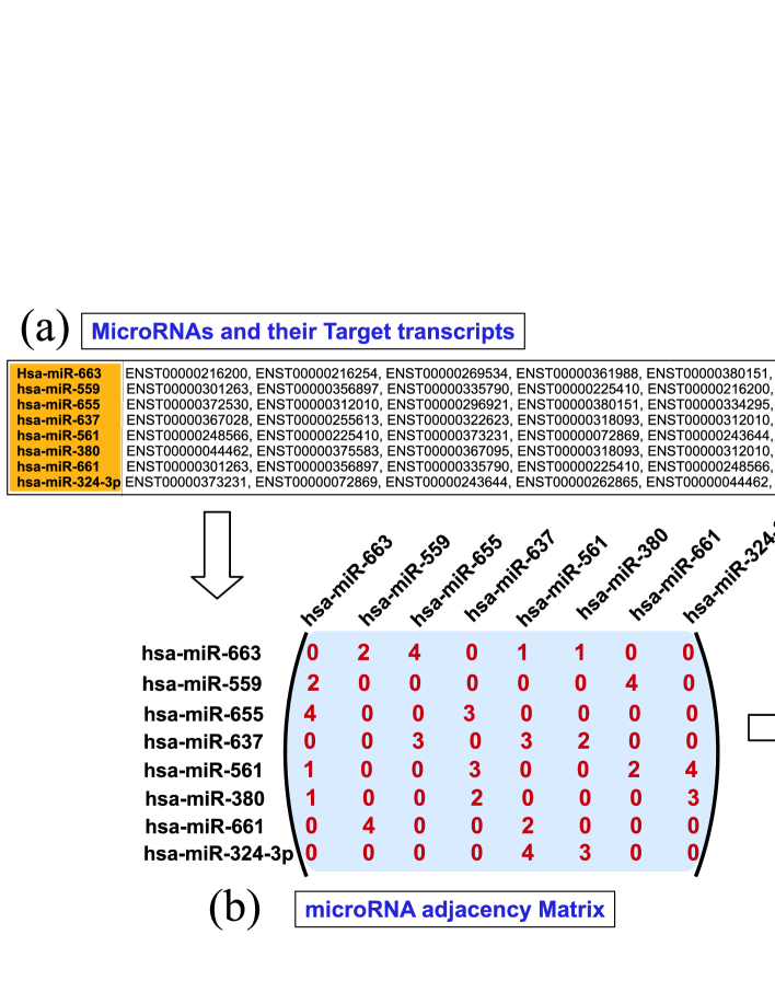
Figure 3: Construction of miRNA co-target network. (a) A representative data for $8$ miRNAs and their targets transcripts. (b) The adjacency matrix ($W$) with elements $W_{ij}$ corresponding to the number of common target transcripts. (c) The miRNA co-target network, where the miRNAs are represented as nodes which are connected by links having weight $W_{ij}.$

4.1 Construction of miRNA co-target network

The miRNAs which act as secondary regulators can target more than one mRNA transcripts and a transcript can also be targeted by many miRNAs. Computationally predicted targets of miRNAs for different species are available in Microcosm Target database [38]. For constructing the miRNA network the targets of miRNAs are collected from the above mentioned database. The data predicts $34788$ targets for $711$ miRNAs for Homo sapiens.

The miRNA co-target network is constructed by considering miRNAs as nodes, and a link with weight $w$ is connected between two miRNAs if they both target $w$ number of same target transcripts. The detailed procedure for constructing the miRNA co-target network is shown in Fig. 3. The network thus formed is weighted and undirected. For convenience, miRNAs are given arbitrary, but unique, identification numbers $m=1,2,\dots i,\dots M,$ where $M$ represents the total number of miRNAs present in the species. The miRNA network is represented as adjacency matrix $W,$ where a element $W_{ij}$ represents the number of mRNAs co-targeted by miRNA $i$ and $j$ together. Thus $W_{ij}$ represents the weight of the link joining the nodes $i$ and $j.$ If a miRNA pair $i$ and $j$ have no common targets, they are not connected and we set $W_{ij}=0.$ The diagonal elements of matrix $W$ are taken to be zero $i.e.,$ $W_{ii}=0.$ The link-weights of the miRNA co-target network can not be ignored while finding the communities present in the network; the community structure depends on both weights and the connectivity of the miRNAs.

Figure 4: The plot of $q$ verses the number of components ($N(q)$) show a monotonically increasing curve. At every $q$ the partition of the network correspond to a modularity value $M(q)$. The plot of modularity $M(q)$ verses $q$ shows a peak at $q=q_{c}(=146).$

Size	Freq
1	284
2	47
3	24
4	8
5	6
6	5
9	1
12	1
16	1
47	1
85	1

Table 1: The distribution of size of the components at $q_{c}$$=$$146$ for miRNA co-target network of Homo sapiens.

4.2 Results

We obtain the components of miRNA co-target network by progressively deleting the links which have weight less than $q.$ For each $q,$ taking the components as the communities of the graph, we calculate modularity $M(q).$ Figure 4 shows $N(q)$ and $M(q)$ as a function of $q.$ As expected $N(q)$ is non-decreasing function whereas $M(q)$ shows a maximum at $q_{c}=146.$ Here, the maximum modularity is $M(q_{c})=0.044$ and there are $379$ components, of which $284$ are isolated miRNAs and the rest $95$ have two or more miRNAs each (for details refer to Table. 1). Clearly, most of the components contain small number of miRNAs (less than $7$), some have moderate number $(9,12,16)$ and only two are large containing $47$ and $85$ miRNAs.

Module size :	2	3	4	5	6	7	9	11	12	13	14	19	21
Frequency :	65	38	4	5	1	1	3	1	2	1	1	1	1

Table 2: Size distribution of miRNA modules obtained using the algorithm proposed in this work. Note that there are $284$ number of lone miRNAs which are not shown here.

In the next step we aim at finding modules of all these $95$ disjoint graphs individually using NGM algorithm for weighted network [34] to each of them. It turns out that only the large and moderate sized components give rise to smaller substructures (modules). For example, the largest component (I in Fig. 5) containing $85$ miRNAs, partitions into $7$ small modules of size $(14,12,12,19,11,13,4)$ and the next largest having $47$ miRNAs (II in Fig. 5) has $6$ modules of size $(9,21,3,3,2,9).$ Partition of other three components of size $16,12$ and $9$ are also shown in Fig. 5 ( marked as III, IV and V respectively). As a whole this algorithm results in $125$ modules in total. The distribution of their sizes is given in Table 2.

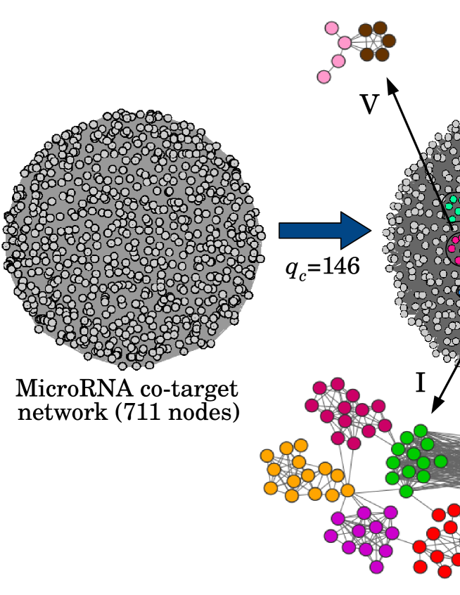
Figure 5: Left:The miRNA co-target network of Homo sapiens; it is fully connected network within $711$ nodes. Right: At $q_{c}=146$ all the components of size more than $5$ obtained are marked with different colours. Top five components are identified with roman numbers, Component I (size : $85$), II $(47)$, III $(16)$, IV $(12)$ and V $(9)$. These components when further analyzed with NGM weighted algorithm they partition into several modules.

The size of the partitions obtained for human miRNA co-target network using (i) NGM algorithm for weighted network [34], (ii) clustering algorithm of Ref. [20] and (iii) the current work are compared in Table 3. It is evident that NGM algorithm gives the highest modularity, but the modules obtained there are very large. On the other hand, the clustering algorithm [20] gives smaller modularity value and moderate size clusters and it was claimed that these clusters are biologically relevant $i.e.,$ they are pathway, tissue or disease specific. However, some of the clusters are still very large, and it is difficult to ascertain functional specificity to these clusters. This problem is resolved in our algorithm in expense of low modularity value. Such partitions can be accepted only when the functional specifications obtained here are consistent with those obtained earlier [20].

In Ref. [20] the authors have obtained $70$ clusters, each having two or more miRNAs. All these clusters are found to be pathways, disease or tissue specific; for convenience, we denote them as $C_{1},C_{2},\dots,C_{70}.$ We analyze the miRNA contents of these $70$ clusters in terms of the $124$ modules obtained in this work (namely $M_{1},M_{2},\dots M_{124}$). If modular structure of miRNAs are different from those of the clusters, one would expect that each cluster would contain miRNAs belonging from many different modules. However we find that each cluster, in terms of their miRNA content, is either identical to one of the modules or composed of at most four modules. This is described in Fig. 6 in details. As described in the Fig. 6, clusters $C_{1}$ to $C_{44}$ are identical to the respective modules $M_{1}$ to $M_{44}$. Module $M_{45}$ is same as $C_{45}$ but contains one extra miRNA, marked as $S$ in Fig. 6; the same is true for modules $M_{46}$ to $M_{55}.$ MicroRNAs of all other clusters $C_{56}$ to $C_{70}$ comes from two or more modules. If all miRNAs of a module participate in forming a cluster we represent it in Fig. 6 by a fully shaded box, or otherwise by a partially shaded box. For example, $C_{60}$ consists of all miRNAs of module $M_{60}$ and some miRNAs of $M_{74}.$ Note that miRNAs of module $M_{49}$ belong to two clusters $C_{49}$ and $C_{69}$; another example is $M_{80},$ whose miRNAs belong to $C_{66}$ and $C_{70}.$

Methods	$N(q)$	Component size	$M(q)$
NGM algo. [34]	$4$	$(6,79,294,332)$	$0.081$
Clustering algo. [20]	$94$	$(1,2,3,4,5,6,7,8,9,11,14,16,31,47)$	$0.025$
This work	$124$	$(1,2,3,4,5,6,7,9,11,12,13,14,19,21)$	$0.022$

Table 3: Comparison of the three methods in context of finding the modules of densely connected weighted miRNA co-target network. The number of components or modules $N(q)$ obtained with the corresponding modularity $M(q)$ are mentioned along with the sizes of the components for each of the algorithms.

This analysis revels that the modules obtained in this work are either same or very similar to those obtained in [20]. Since miRNA clusters are known to be pathway and tissue specific, the modules obtained here, which are combined to form the clusters are also biologically relevant [41].

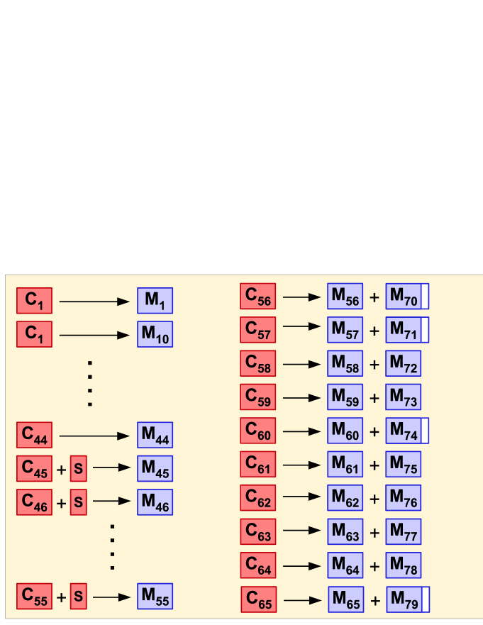
Figure 6: Comparison of the modules obtained using the algorithm of this current work with the clusters got from the clustering algorithm in Ref. [20]. It is clear that all the cluster of miRNAs (denoted as $C$) are just combination of the modules (denoted as $M$) obtained here. The number written as subscript of $C$ and $M$ represents the ID number of the clusters and modules.

5 Conclusion

In this article we propose an algorithm to detect community structure of dense weighted networks. If the network has adjacency matrix $W$ whose elements $W_{ij}$ refer to the weight of the link connecting nodes $i$ and $j$, one can implement the algorithm by the following steps, I. Delete all the links having weight $W_{ij}<q$; find the modularity $M(q)$ of the network taking the disjoint components obtained here as the partitions. II. Find $q_{c}$ where $M(q)$ is maximum. III. Take all the components at $q=q_{c}$ containing two or more miRNAs, one at a time, apply Newman Girvan’s weighted algorithm to obtain its modules. To demonstrate the algorithm, we consider miRNA co-target network of Homo sapiens, which is dense and weighted, and compare the modules with the miRNA clusters obtained earlier [20]. It turns out that most clusters are either identical to one of the modules, or composed of miRNAs belonging to at most four different modules. Thus, like the clusters, modules are also involved in specific biological functions.

This algorithm has certain advantage over some of the standard ones. The NGM algorithm for weighted networks [34] can not resolve small sub-structures if the network is dense. The algorithm of Ref. [20] can overcome this difficulty, but does not resolve communities which are interlinked by a few links having very large weights. The algorithm discussed here combines both the methods suitably and overcome their shortcomings. Unlike the algorithm of [20], where actual number of clusters depends (though weakly) on the final choice of $q$($=160$ in [20]) this algorithm is free from parameters and provide an unique partition of a weighted network.

It has been known that a network containing $l$ connections can not resolve any module which has $\sqrt{l/2}$ links. Usually, a densely connected weighted network, with a wide distribution of link weights falls in this category and it is difficult to resolve small substructures of these networks. We believe the algorithm considered here is general, though discussed in context of miRNA co-target networks, and can be used for community detection in dense and weighted networks.

References

- [1] M. E. J. Newman, Proc. Natl. Acad. Sci. USA 98, 404 (2001).
- [2] J. Moody, Am. J. Sociol 107, 679 (2001).
- [3] G. Bagler, Physica A 387, 2972 (2008).
- [4] S. Lammera, B. Gehlsena, D. Helbinga, Physica A 363, 89 (2006).
- [5] S. H. Y. Chan, R. V. Donner, S. Lmmer, Eur. Phys. J. B 84, 563 (2011).
- [6] P. Sen, S. Dasgupta, A. Chatterjee, P. A. Sreeram, G. Mukherjee, S.S. Manna, Phys. Rev. E 67, 036106 (2003).
- [7] W. Li, X. Cai, Physica A 382, 693 (2007).
- [8] R. Albert, A. L. Barabási Rev. Mod. Phys. 74, 47 (2002).
- [9] M. Newman, A. L. Barabási, D. J. Watts, The Structure and Dynamics of Networks, Princeton University Press 2006.
- [10] M. Girvan, M. E. J. Newman, Proc. Natl. Acad. Sci. U.S.A. 99, 7821 (2002).
- [11] U. Alon, Nat. Rev. Genet. 8, 450 (2007).
- [12] R. Cohen, K. Erez, D. B. Avraham, S. Havlin, Phys. Rev. Lett. 85, 4626 (2000).
- [13] J. R. Banavar, A. Maritan, A. Rinaldo, Nature 399, 130 (1999).
- [14] R. Cohen, S. Havlin, Complex Networks: Structure, Robustness and Function, Cambridge University Press, Cambridge, 2010.
- [15] M. E. J. Newman, Phys.Rev. E 64, 016131 (2001); M. E. J. Newman, Phys. Rev. E 64, 016132 (2001).
- [16] G. Fagioloa, J. Reyesb, S. Schiavoc, Physica A 387, 3868 (2008).
- [17] A. D. Montis, M. Barthelemy, A. Chessa, A. Vespignani, Environ. Plann. B 34, 905 (2007).
- [18] A. Barrat, M. Barthélemy, R. P. Satorras, A. Vespignani, Proc. Natl. Acad. Sci. U.S.A. 101, 3747 (2004).
- [19] J. M. Kumpula, J. P. Onnela, J. Saramäki, K. Kaski, János Kertész, Phys. Rev. Lett. 99, 228701 (2007).
- [20] S. Mookherjee, M. Sinha, S. Mukhopadhyay, N. P. Bhattacharyya, P. K. Mohanty, Online J Bioinform. 10, 280 (2009).
- [21] S. Wasserman, K. Faust, Social Network Analysis, Cambridge University Press, Cambridge, 1994.
- [22] Y. Kajikawa, J. Ohno, Y. Takeda, K. Matsushima, H. Komiyama, Sustain Sci. 2, 221 (2007).
- [23] R. Guimerá, D. B. Stouffer, M. S. Pardo, E. A. Leicht, M. E. J. Newman, L. A. N. Amaral, Ecology 91, 2941 (2010).
- [24] E. L. Rezende, E. M. Albert, M. A. Fortuna, J. Bascompte, Ecology Letters 12, 779 (2009).
- [25] P. Holme, M. Huss, H. Jeong, Bioinform. 19, 532 (2003).
- [26] E. Ravasz, A. L. Somera, D. A. Mongru, Z. N. Oltvai, A. L. Barabási, Science 297, 1551 (2002).
- [27] B. W. Kernighan, S. Lin, Bell Syst. Tech. J. 49, 291 (1970).
- [28] M. Fiedler, Czech. Math. J. 23, 298 (1973).
- [29] A. Pothen, H. Simon, K. -P. Liou, SIAM J. Matrix Anal. Appl. 11, 430 (1990).
- [30] J. Scott, Social Network Analysis: A Handbook, 2nd ed. (Sage,London, 2000).
- [31] M. E. J. Newman, M. Girvan, Phys. Rev. E 69, 026113 (2004).
- [32] M. E. J. Newman, Phys. Rev. E 69, 066133 (2004).
- [33] A. Clauset, M. E. J. Newman, C. Moore, Phys. Rev. E 70, 066111 (2004).
- [34] M.E.J. Newman, Phys. Rev. E 70, 056131 (2004).
- [35] S. Fortunato, M. Barthélemy, Proc. Natl. Acad. Sci. USA 104, 36 (2007).
- [36] M. Basu, N. P. Bhattacharyya, P. K. Mohanty , J. Phys.: Conf. Ser. 297, 012002 (2011).
- [37] K. K. Farh et. al., Science 310, 1817 (2005).
- [38] Microcosm Targets :www.ebi.ac.uk/enright-srv/microcosm/htdocs/targ ets/v5/.
- [39] N. J. Clarke, P. Sanseau, MicroRNA: Biology, Function and Expression, DNA Press, 2007.
- [40] J. Xu et. al. Nucleic Acids Res. 39, 825 (2010).
- [41] An independent study of biological relevance of these modules will be reported elsewhere.