THE AGILE ALERT SYSTEM FOR GAMMA-RAY TRANSIENTS

Abstract

In recent years, a new generation of space missions offered great opportunities of discovery in high-energy astrophysics. In this article we focus on the scientific operations of the Gamma-Ray Imaging Detector (GRID) onboard the AGILE space mission. The AGILE-GRID, sensitive in the energy range of 30 MeV$-$30 GeV, has detected many $\gamma$-ray transients of galactic and extragalactic origins. This work presents the AGILE innovative approach to fast $\gamma$-ray transient detection, which is a challenging task and a crucial part of the AGILE scientific program. The goals are to describe: (1) the AGILE Gamma-Ray Alert System, (2) a new algorithm for blind search identification of transients within a short processing time, (3) the AGILE procedure for $\gamma$-ray transient alert management, and (4) the likelihood of ratio tests that are necessary to evaluate the post-trial statistical significance of the results. Special algorithms and an optimized sequence of tasks are necessary to reach our goal. Data are automatically analyzed at every orbital downlink by an alert pipeline operating on different timescales. As proper flux thresholds are exceeded, alerts are automatically generated and sent as SMS messages to cellular telephones, e-mails, and push notifications of an application for smartphones and tablets. These alerts are crosschecked with the results of two pipelines, and a manual analysis is performed. Being a small scientific-class mission, AGILE is characterized by optimization of both scientific analysis and ground-segment resources. The system is capable of generating alerts within two to three hours of a data downlink, an unprecedented reaction time in $\gamma$-ray astrophysics.

1 Introduction

Gamma-ray astrophysics above 100 MeV from space have substantially progressed in recent years. After a first pioneering phase, space observatories such as COS-B ( from 1975 to 1982; Mayer-Hasselwander (1979); Swanenburg et al. (1981)) and the Compton Gamma-Ray Observatory (CGRO; from 1991 to 2000; Fichtel & Trombka (1997)) were able to successfully map $\gamma$-ray sources and extended Galactic regions. The field of view (FoV) of the $\gamma$-ray instrument EGRET onboard of CGRO and operating in the 100 MeV$-$10 GeV domain was sufficiently large enough (0.5 sr) to simultaneously monitor many sources in the Galactic plane and at high Galactic latitudes Fichtel & Trombka (1997); Thompson et al. (1993). The EGRET point-spread function (PSF; 6$-$7^∘ for the 68% containment radius at 100 MeV) allowed a first mapping of the Galactic plane and source positioning. Today, with the advent of silicon-based $\gamma$-ray detectors AGILE Tavani et al. 2009a and Fermi-LAT Atwood et al. (2009), both the PSF and FoV have substantially improved since the 1990’s. For both AGILE and Fermi-LAT, the FoV is now quite large (about 2.5 sr), covering more than 1/5 of the whole sky, and the PSF at 100 MeV has a containment radius of 3$-$4^∘ Abdo et al. (2009); Chen et al. (2013). Large portions of the sky can then be simultaneously monitored with optimal source detection capabilities. The issue of optimizing source monitoring and the search for $\gamma$-ray transients is thus of great importance.

AGILE (Astrorivelatore Gamma ad Immagini LEggero $-$ Light Imager for Gamma-ray Astrophysics) is a scientific mission of the Italian Space Agency (ASI) that was launched on 2007 April 23 Tavani et al. 2009a . The Gamma-Ray Imaging Detector (GRID) is used for observations in the 30 MeV$-$30 GeV energy range. The AGILE orbital characteristics (quasi-equatorial with an inclination angle of 2^∘.5 and an average altitude of 530 km, $96^{\prime}$ period) are optimal for low-background $\gamma$-ray observations. From 2007 July to 2009 October, AGILE observed the $\gamma$-ray sky in the so-called “pointing mode”, which is characterized by quasi-fixed pointings with a slow drift ($\sim 1^{\circ}$/day) of the instrument boresight direction following solar panel constraints. Due to a change in the satellite pointing system control, since 2009 November the AGILE $\gamma$-ray observations have been obtained with the instrument operating in “spinning mode” ( i.e., the satellite axis sweeps a 360^∘ circle in the sky every approximately $7^{\prime}$). Depending on the season, the whole sky is progressively exposed.

The variability aspect of the $\gamma$-ray sources is a key factor for our understanding of their origin and nature Ackermann et al. (2013); Hinton & Starling (2013), and the study of the variability of the $\gamma$-ray sky above 30 MeV requires special focusing and resources. The task can be daunting: a large fraction of currently known $\gamma$-ray sources are unidentified, and in general many sources show statistically significant variability at all timescales (hours, days, weeks).

The $\gamma$-ray transient monitoring program is a very important task of the AGILE science program. It became active in a preliminary fashion at the beginning of the mission ( the summer of 2007) and it has been improving ever since. It is a dedicated alert system that is implemented within the AGILE Ground Segment. Because detecting time variable sources during their early phases of emission and fast communication with the astrophysics community are crucial, the AGILE Alert System s goal is to provide excellent quality $\gamma$-ray data within the shortest time possible for scientific analysis and follow-up observations. This task requires a necessarily automated detection system that can issue alerts immediately upon detection of $\gamma$-ray flares, enabling then the study of the transient sky. In this article, we focus on the innovative features of the scientific analysis performed at the AGILE ground segment level. In particular, we describe the successful strategy for fast analysis of $\gamma$-ray data, a challenging task that requires a special optimization of resources (Section 2). We also discuss the role played by special software tools and algorithms (Section 3). Section 4 presents the team organization and the tools developed for mobile devices to support the manual procedures to confirm automatic alerts. Section 5 focus on the characterization of the statistical significance of pipeline alerts. Section 6 summarizes some of the scientific results provided to the astrophysical community; we discuss, as a concrete example, the reaction time for the very important case of the 2010 Crab Nebula $\gamma$-ray flare discovered by AGILE.

The main goals of this article are to describe: (1) the AGILE Alert System, focusing on the pipeline developed at IASFBO; (2) a new algorithm (“spotfinder”) for blind search identification of flare candidates within a short processing time; (3) the AGILE procedure for alert management; and (4) an evaluation of the statistical distribution of the data products in order to properly evaluate the false detection occurrence rate.

2 General overview

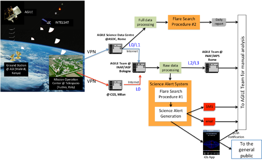
Figure 1: General architecture of the Ground Segment with details of the online AGILE Alert System (green boxes indicate the data processing, and orange boxes indicate the most specific pipelines for $\gamma$-ray flare search and alert generation) in terms of nodes of elaboration and functional blocks. The arrows indicate the data flow between different nodes and functional blocks.

This section describe the general architecture of the AGILE Ground Segment from data acquisition to alert generation (see Figure 1).

AGILE data are downlinked to the ASI Malindi ground station in Kenya every orbit (about every 96 minutes which is the time window for data retrieval, and commands transmitting is 10 minutes per orbit). Data are then quickly transferred via ASINet through a dedicated Intelsat bidirectional link to Telespazio, Fucino (AQ, Italy), where the Mission Operation Center (MOC) is located. Data are then transferred to the ADC, which is located in Frascati (Italy), for data reduction, archiving, and distribution.

Raw data are routinely archived at the ADC, and then converted to FITS format L1 ( preprocessed data) through the AGILE Preprocessing System Trifoglio et al. (2008). Data are further processed (L2, or event list and L3, or sky maps) using software tasks developed by the AGILE instrument team and then integrated into the pipeline systems developed at ADC for quicklook monitoring and consolidated archive generation. The L0 and L1 data are forwarded to the IASFBO site Trifoglio et al. (2007) where the IASFBO SAS pipeline runs.

The AGILE Alert System is composed of two independent automated analyses parts: (1) the Quick-Look Scientific (QLS) pipeline running at the AGILE Data Center (ADC) (hereafter ADC QLS pipeline), which is part of the ASI Science Data Center (ASDC); and the (2) AGILE-GRID Science Alert System (SAS) pipeline running at the INAF/IASF Bologna (IASFBO) (hereafter IASFBO SAS pipeline). These systems process the data with different levels of data processing and procedures while looking for transient $\gamma$-ray events. Both systems operate in real-time mode, with automatic processing starting as soon as data are available. The IASFBO SAS pipeline generates an alert to the AGILE Team for each candidate $\gamma$-ray flare within two to three hours from the time of the last orbit data acquisition stored in the satellite. In doing so, preference is given to speed rather than completeness of orbital telemetry. On the other hand, ADC QLS pipeline generates a daily report containing a list of candidate flares, sent via e-mail using a more complete data archive.

The final consolidated archive of the AGILE Mission is then produced at ADC by a dedicated pipeline.

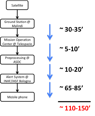
Figure 2: Data transfer time of the Ground Segment from the AGILE satellite to SMS of scientific alerts to mobile phones.

As data of the latest acquired orbit are received at the IASFBO site, data processing by the IASFBO SAS pipeline starts immediately running on a cluster system of 64 CPUs. Processing time typically lasts about $65^{\prime}$$-$$85^{\prime}$ in order to analyze in parallel all accessible sky regions, taking into account the $\gamma$-ray exposure. In order to detect transients or variable sources the Flare Search Procedure 1 subsystem performs an automated search for transient $\gamma$-ray emission. The output is then analyzed to select the best transient candidates. Details on the time duration required to perform each step of data transfer and elaboration are reported in Figure 2.

Another independent subsystem, (the Flare Search Procedure 2), is part of the ADC QLS pipeline. The procedure uses a more complete data set to consolidate the data of the current orbit. The procedure is necessarily slower (it requires about 3.5 to 5 hours after data acquisition), as it is necessary to wait the following orbit to generate an output, because the data to reconstruct the last minutes of the satellite pointing direction are contained in the next orbit). The ADC result is in the form of a daily report that lists all candidate $\gamma$-ray transients, and it is distributed via e-mail to the team twice a day.

When the AGILE Team receives a high confidence automatic alert from the IASFBO SAS pipeline, a more refined analysis is undertaken before communication to the astronomical community. A visual check of counts and intensity maps is performed via a web browser and also through smartphones. The alert is analyzed in parallel with the online data archives of both ADC and IASFBO: the IASFBO site acts also as a point of distribution to the AGILE Team Center (ATC) (located at INAF/IAPS, Rome) of the L2 and L3 data generated by SAS itself. This L2/L3 operative archive is used in the daily quick-look monitoring activities.

A dedicated Application (App) for smartphones and tablets (the AGILEScience App) is also connected with the IASFBO SAS pipeline and has a reserved area where the scientific results are made visible to the AGILE Team. Processed results can also be made available to the public through this App (see Section 4.1.1).

3 The IASFBO SAS Analysis Procedure

The Flare Search Procedure 1 of the IASFBO SAS pipeline automatically performs a search for transient $\gamma$-ray emissions in two steps:

1. a selection of an ensemble of models of transient sources (i.e., a selection of a list of candidate $\gamma$-ray flaring sources ) with two independent methods: a blind search procedure called spotfinder (see Section 3.2) and the use of a list of known sources from selected astrophysical source catalogues; and

2. calculation of the flux and significance level for each $\gamma$-ray transient candidate (see Section 3.3) .

This procedure produces a list of candidate flares with its associated statistical significance. Alerts are generated for a subclass of these selected candidates (see Section 3.4).

Data are analyzed for each orbit, producing a sliding window in the generated light-curves of $\gamma$-ray sources. An example is reported in Figure 3.

3.1 Data Analysis Method

The AGILE-GRID data analysis is currently performed on the data set generated with the software package (version 4) publicly available at the ASDC website and uses the FM3.119 background event filter (see A. Bulgarelli et al. (2014, in preparation)) and the I0023 version calibration matrices (Chen et al., 2013). The events collected during the passage in the South Atlantic Anomaly and Earth albedo background photons are removed from the pipeline. To reduce particle background contamination, we select only events flagged as confirmed $\gamma$-ray events ( G-class events, corresponding to a sensitive area of $\sim$ 330 cm² at 100 MeV). AGILE counts, exposure, and Galactic diffuse emission background maps are generated with a bin size of $0^{\circ}.3\times 0^{\circ}.3$ to compute the period-averaged source flux and its evolution.

Owing to the relatively low event detection rate and the extent of the AGILE-GRID PSF, a binned multisource Maximum Likelihood Estimator (MLE) developed at INAF/IASF Milano is used to search for transient emission from $\gamma$-ray sources. This method iteratively optimizes the position and flux of all the sources of the region Bulgarelli et al. 2012b . The use of a binned likelihood method greatly increases the speed of analysis with respect to an un-binned version. The possibility to optimize at the same time source flux and position has simplified the development of the pipeline. The same tool is used also in the manual verification procedure (see Section 4).

The likelihood ratio test $T_{s}$ calculated by the MLE is used to compare two ensembles of hypotheses, one in which a $\gamma$-ray source is present and another (the null hypothesis) in which it is absent. More specifically, the null hypothesis can be formulated as an ensemble of models that keep the flux of the flaring source fixed to zero and the fluxes of steady sources fixed to their known fluxes (if any). For the alternative hypothesis (a flaring source is present), the flux and position of this source are allowed to be free, and the fluxes of steady sources are fixed to their known fluxes. The analysis is performed over a region of $10^{\circ}$ radius. The Galactic diffuse $\gamma$-ray radiation Giuliani et al. (2004) and the isotropic emission are taken into account in the model with two parameters: (1) $g_{gal}$, the coefficient of the Galactic diffuse emission model, and (2) $g_{iso}$, the isotropic diffuse intensity. As noted in (Bulgarelli et al. 2012b, ) the isotropic component is dominated by instrumental charged particle background rather than by the extragalactic diffuse emission, in contrast to data from EGRET and Fermi-LAT. This instrumental charged particle changes over time and space and for these reasons they are kept free during the data analysis.

We analyze the sky within the current AGILE FoV over one-day intervals during the “pointing mode” period and over two-day intervals during the “spinning mode” period to obtain approximately similar exposures for both “pointing” and “spinning” at the center of the exposed region. We identify the transient episodes, analyzing both the 100 MeV$-$30 GeV and 400 MeV$-$30 GeV energy bands.

3.2 Automated Blind Search for Transient $\gamma$-Ray Emissions

The peculiarity of the AGILE-GRID instrument has required the development of a new algorithm called spotfinder that extracts “candidate $\gamma$-ray flares” from Gaussian smoothed $\gamma$-ray sky maps (either counts or intensity maps are used); the automated blind search for transient $\gamma$-ray emission procedure is based on this algorithm, that takes into account the following issues:

1. The FoV of the AGILE-GRID instrument usually contains both the Galactic plane and the extra-Galactic sky, that are very different in terms of

   1. background components (the Galactic plane is dominated by the diffuse $\gamma$-ray emission, the extra-Galactic sky is dominated by the isotropic emission);

   2. the number of $\gamma$-ray sources in the same area of the sky.

2. the AGILE-GRID instrument has a PSF of 2^∘.1 at 30^∘ off-axis for $E>100$ MeV reconstructed energy (and spectral index $\alpha=-1.66$ from Monte Carlo data). This algorithm takes into account this extension;

3. due to the fact that the isotropic component is dominated by the charged particle background that may change over space, the spotfinder algorithm estimates the background components (diffuse, isotropic and instrumental) for each sub-region of the $\gamma$-ray sky map.

The development and optimization of this algorithm was one of the main tasks for the development of our automated data analysis system for detection of $\gamma$-ray flares. Spotfinder is basically a connected component labeling algorithm (Rosenfield & Pfaltz, 1966) that works with multilevel images. Each $\gamma$-ray emission can be viewed as a connected component region. It uses a labeling algorithm Di Stefano & Bulgarelli (1999) that searches for the connected regions in a binary image (an image with two colors, black and white).

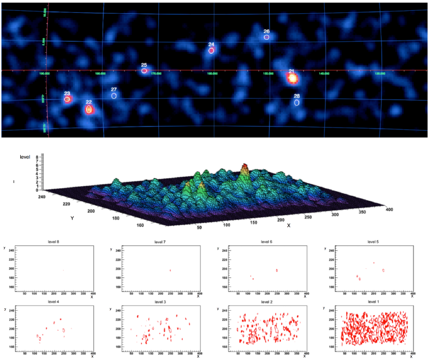
Figure 4: spotfinder algorithm for the extraction of connected regions into a multilevel $\gamma$-ray map. Top panel: a region of the Galactic plane used as an example; also shown in the same picture are the connected component regions identified by spotfinder. Second panel: the same sky region normalized in eight levels. Third panel: the eight images used to grow the connected regions.

Each counts or intensity map is segmented into three different regions ($b<-10^{\circ}$, $|b|<10^{\circ}$, and $b>10^{\circ}$) to account for the higher background and source confusion near the Galactic plane (see first panel of Figure 4). After the selection of a sky region, there are some options that can change the value of the pixels: (1) if the value of a pixel is above a well-defined threshold, it is set to zero to maximize the effectiveness of the search in regions with a low $\gamma$-ray emission; (2) if the value of the exposure is below a threshold, the related pixel in the counts or intensity maps is set to zero to avoid searches in sky regions with a low level of exposure; and (3) it is possible to subtract two maps. In the current version of the algorithm used in the IASFBO SAS pipeline, only option (2) is used with a typical value of 50 cm^-2 s sr for maps with a bin size of 0^∘.3.

A Gaussian smoothing of the map is performed with a typical kernel of three bins. In a $\gamma$-ray smoothed map the values of a pixel range from 0 to a maximum value within a continuous interval of values. After smoothing, the intervals are normalized and discretized to $N$ intervals, which rounds each value to the nearest integer value (see the second panel of Figure 4) and divides the original image into $N$ images ($N$=100 is a typical value) containing only pixels with the same value $k$ (see the third panel of Figure 4 with $N=8$). The connected component search procedure starts from these normalized and discretized maps.

The search for connected component regions is an iterative procedure. The procedure starts by considering only the image that contains the pixels with value $N$ and then by calculating the connected component regions contained into this first image. For each iteration $k$ ($k=N-1,$…$,1$) the level $k-1$ is added to the current image, and new connected component regions are calculated. The effect of merging two levels is that the original regions grow by adding the pixels of the neighboring level. This growing procedure stops when more than $M$ connected regions are found (where $M$ is a parameter, a typical value is 8). At the end, for each connected region the barycenter is calculated. This is the starting position for the MLE (see an example of the found connected regions in the first panel of Figure 4).

There are also some additional options that are applicable after the determination of the connected regions: (1) if two connected regions are too close, only the first connected region survives; and (2) if a connected region is outside a circle centered in the center of the map with a radius specified by the user, this region is discarded.

3.3 Calculation of the Significance of Each Candidate Flare

The second step of the automated search procedure for transient $\gamma$-ray emission is the calculation of the confidence level of each candidate flaring source, which is performed in two substeps using the MLE. In the first substep, all sources included in the initial ensemble of models (ordered using the intensity value of the bins contained in the connected region and above a predefined exposure level threshold) are analyzed; the flux of the candidate flares is allowed to vary and the position is kept fixed at the value of the center of the connected region. This step is useful to reduce the number of candidates for the final evaluation, which minimizes the complexity of the model. In the final step, only detections with $\sqrt{T_{s}}\geq 2$ are selected and reanalyzed simultaneously. The flux and position of the candidate flares are allowed to vary, and the spectrum of each candidate is assumed to be a power law with the spectral index kept fixed to 2.1. In the end, we obtain a list of candidate transient sources and their pretrial statistical significance.

3.4 Science Alert Generation

For each candidate transient event with $\sqrt{T_{s}}>25$ (corresponding to $\sigma\geq 4.3$; see Section 5) an alert is generated and sent via SMS, e-mail and through the notification system of the iOs AGILEScience App (see Section 4.1.1).

The generated e-mail contains the following information:

• counts, flux, and related errors;

• the optimized position of the source, error circle, and ellipse at $95\%$ confidence levels;

• a list of possible associations within the error circle based on a list of known sources;

• a short description of the parameters of the analysis;

• the exposure value;

• some useful links to NED and SIMBAD to check the presence of known sources within the error circle;

• a link to the web directory containing the analyzed data and the overall results; and

• the detailed result of the run resulting in a detection (the overall list of sources and the background estimation parameters are provided).

The SMS and the App notifications contain a reduced version of the e-mail content. These notifications only include the significance level, the flux and related error, the exposure level, a possible association, and the list of analysis parameters.

4 The Final Verification Procedure

For the most interesting automatic detections, a final verification is performed by human intervention. During routine daily monitoring, two scientists on duty are assigned to check the alerts generated by the IASFBO SAS pipeline, one from the AGILE Team (at INAF IASF Bologna, Milan, Palermo, IAPS Rome, and INFN Trieste) and one at the ASDC. Alerts automatically generated by the IASFBO SAS pipeline are cross-checked with the data and daily reports generated by the ADC QLS pipeline. The alerts generated by the IASFBO pipeline are received about two hours before the high quality L2 data generated by the ASDC pipeline, and this enables the AGILE Team to gain time during the final check.

This is a key point of the overall AGILE Alert System. We can perform a check before the refined version of the scientific data is available. We can then optimize the results of this analysis with the IASFBO raw data archive, and check the results with the ADC consolidated archive when available. Both pipelines work with the common goal of producing scientific results in the shortest possible time and with the best data quality. Only detections of pretrial significance larger than $5\sigma$ (see Section 5) that survive this check by human intervention are candidates for fast alerts to be distributed to the community. The significance threshold might occasionally be lower if there is independent evidence of simultaneous activity from a reliable counterpart source at other wavelengths.

The final verification is basically divided into (1) a visual inspection of the AGILE sky maps (see Section 4.1), and (2) a data analysis by human intervention (see Section 4.2).

4.1 Quick Look of Sky Maps

When an automatic candidate alert is received, the first step performed during the monitoring activity is the quick look of the data products (e.g., maps and light curves) through web pages accessible via a web browser for personal computers or smartphones and via the AGILEScience App.

4.1.1 The AGILEScience App

To support the management of candidate alerts, an iOS App (the AGILEScience App) has been developed at IASFBO by the AGILE Team in collaboration with the University of Modena and Reggio Emilia. This app consists of (1) a public section with outreach purposes, (2) a private section, and (3) a notification system that sends the AGILE-GRID alerts to the AGILE Team. Furthermore, the App notification system generates also alerts (to everyone, not only to AGILE Team) when a new Astronomical Telegram or GCN circular is published.

In the public section, the last available full sky $\gamma$-ray map can be seen by the public for scientific and outreach purposes in order to follow the evolution of the $\gamma$-ray sky as detected by AGILE (the map is updated every AGILE orbit). This means that also the non-professional astronomer can follow the $\gamma$-ray sky ’in real-time’. All the public content of the AGILEScience App is also available through a web browser for Android mobile devices.

The private section is password protected and shows the analyzed data, in particular, (1) zoomable full sky maps and the analyzed regions overlapped with the automated results provided by IASFBO SAS pipeline, and (2) data quality reports provided by ADC QLS pipeline.

The App for mobile devices is deeply integrated into a scientific ground segment and it is used for daily scientific activities. When an automatic candidate alert is received through the notification system, the private section of the App can be used to access the AGILE-GRID maps to check the automated results or the quality of the data.

4.2 Final Analysis

To confirm or to improve the automated analysis results before the publication of an ATel, an analysis by human intervention is performed for a subclass of candidate transient events following the same data analysis strategy as reported in Section 3.1. This analysis is performed taking into account all known sources in the transient region, and uses the most updated version of the AGILE $\gamma$-ray source catalog. For the known sources, we use fixed positions and fluxes in the likelihood analysis. We then add to this ensemble of known sources a point-like source representing the transient candidate initially using the position as determined by the IASFBO SAS pipeline. We then perform the likelihood analysis, initially setting the position and flux of this transient candidate free.

In addition, we first estimate the $g_{gal}$ and $g_{iso}$ parameters with a longer timescale integration (typically 15 days of integration). We then fix them for the short timescale analysis, assuming that these parameters do not vary significantly on timescales on orders of hours-days. Typically, the integration time we use for this final analysis is the same as for the automatic analysis ( one to two days). However, we vary the integration time for timescales smaller than one day to find the $\gamma$-ray flare peak.

5 Statistical Significance of IASFBO SAS Pipeline Data Analysis Technique

In this section, we discuss the methods used to determine the statistical significance of our procedure. Our method is characterized by adding data for the map analysis by a “1-orbit sliding window offset”. This procedure implies that the 15 maps generated every day are not independent from one another, and our statistical analysis has to take this fact into account. This is a very different approach than the one taken by Bulgarelli et al. 2012b , which required a new evaluation of the pretrial significance of a detection and new simulations. In the end, final results are quite similar but the hypothesis of Bulgarelli et al. 2012b and of this article are different from a statistical point of view. For the same reason, the evaluation of the posttrial probability of Bulgarelli et al. 2012b has to be redone and is not valid in this context.

On the basis of the current AGILE-GRID performance in orbit Chen et al. (2013), which is characterized by a relatively large effective area at 100 MeV and a very large FoV, we determine the range of the pretrial test statistic $T_{s}$ in terms of the probability of false detections (the $p$-value) of the automated analysis procedures. The $T_{s}$ is defined as -2 ln ${L_{0}}/{L_{1}}$ where $L_{0}$ and $L_{1}$ are the maximum value of the likelihood function for the null hypothesis and the alternative hypothesis, respectively.

The data is analyzed each orbit, and we reanalyze the data of the 48-hr period (in “spinning” mode) ending with the current orbit. This procedure implies a sliding window offset by one orbit. The specific search (whether a “blind” search or a search for a specific source) has a direct influence on the proper statistical treatment.

5.1 Statistical Significance of the Blind Search Procedure for Unknown Transient Sources

First we address the blind search procedure: the flaring source is unknown, and the position and flux parameters of each candidate are allowed to be free and optimized with respect to the input data. The starting $(l,b)$ position is determined with the already described method called spotfinder.

The determination of the likelihood ratio distribution in the case of the null hypothesis is used to evaluate the occurrence of false detections. To evaluate the $p$-value of the sliding window approach, we performed simulations of empty Galactic regions (i.e., without steady or flaring source). The simulated observations were generated by adding Poisson-distributed counts in each pixel while considering the exposure level, the Galactic diffuse emission model, and the isotropic diffuse intensity. To simulate the sliding window, we simulated 60 exposure and counts maps of $96^{\prime}$ of AGILE orbit for each run (corresponding to four days of observation, 15 orbits for each day). We then added the first 30 of these maps to obtain a two-day observation map; we then removed the first and added the next $96^{\prime}$ map, and so on. Each two-day generated maps (counts, exposure, and Galactic emission maps) have been analyzed using the same procedure as the on-orbit data. Simulated data are generated using the AGILE-GRID instrument response functions I0023 Chen et al. (2013). The parameters used in the simulation are $g_{gal}$ = 0.6 and $g_{iso}$ = 8 (typical of the GRID data processing). During the analysis the spectra of all sources in the field are kept fixed.

We then calculate the $p$-value distribution, analyzing at the same time one, three and eight candidate flares (as upper limits) in an empty field, with the flux and position of each source allowed to vary. Table 1 reports the performed simulation and related parameters.

The probability that the result of a trial in an empty field has $T_{s}\geq h$ is

$$P(T_{s}\geq h)=\int_{h}^{+\infty}\varphi(x)dx$$ (1)

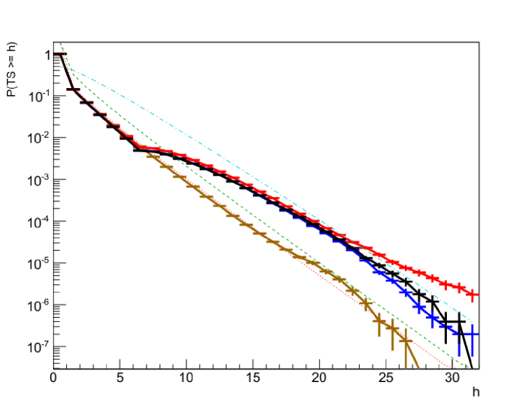
Figure 5: Histograms are the p-value distributions for an empty Galactic region with a different number of candidate flare in the ensemble of models. Each histogram shows the p-value distribution of the first candidate in the ensemble of models (the blue histogram has one candidate, the red histogram has three candidates, and the black histograms has eight candidates). The flux and position of the sources are left free; $g_{\rm gal}$ and $g_{\rm iso}$ parameters are free. The brown histogram shows the p-value distribution for one candidate in the ensemble of models with its position kept fixed. The red dotted line is the $\frac{1}{2}\chi^{2}_{1}$ theoretical distribution, the green dashed line is the $\chi^{2}_{1}$ theoretical distribution, and the cyan dot-dashed line is the $\frac{1}{2}\chi^{2}_{3}$ distribution.

which is also called the $p$-value $p=P(T_{s}\geq h)$. This is the pre-trial type-1 error (a false positive, rejecting the null hypothesis when in fact it is true); the “$p$-value” assigned to a given value of a random variable is defined as the probability of obtaining that value or larger when the null hypothesis is true. The resulting $p$-value distributions are shown in Figures 5$-$7. We fit these distribution with the function,

$$\kappa^{\prime\prime}(T_{s})=\left\{\begin{array}[]{ll}\delta&\mbox{if }T_{s}<1\\ \eta_{1}\chi^{2}_{N_{1}}(T_{s})&\mbox{ if $T_{s}\geq 1$ and $T_{s}\leq t_{lcl}$ }\\ \eta_{2}\chi^{2}_{N_{2}}(T_{s}-t_{lcl})&\mbox{ otherwise }\end{array}\right.$$ (2)

where $t_{lcl}$ is a threshold that enables the location of the contour level: a typical value is $t_{lcl}=5.99147$, which corresponds to a 95% confidence level for two degrees of freedom. We find that $N_{1}$ = 1 (if $T_{s}<t_{lcl}$, no optimization of the position takes place, and the only free parameter is the source flux), $N_{2}=5$, and the remaining parameters depend on the hypothesis; Table 2 reports results for some cases. As already stated, similar results have been obtained by the analysis of an empty Galactic region with no sliding window (Bulgarelli et al. 2012b, ) but under different hypothesis.

Fitting the distribution of the $g_{gal}$ and $g_{iso}$ parameters with a Gaussian distribution, we obtain $g_{gal}=0.68\pm 0.15$ and $g_{iso}=8.1\pm 2.7$. Similar results have been obtained for eight sources in the ensemble of models.

5.2 Statistical Significance of the Search Procedure for Transient Emission from Known Sources

In the following section, we address the search for a specific transient source using a list of known $\gamma$-ray sources in the region. The main difference between this procedure and the blind search procedure already described is that the source positions are kept fixed, and only the fluxes are allowed to vary. Fitting these distribution with the function,

$$\kappa^{\prime}(T_{s})=\left\{\begin{array}[]{ll}\delta&\mbox{ if $T_{s}<1$},\\ \eta\chi^{2}_{N_{1}}(T_{s})&\mbox{ otherwise, }\\ \end{array}\right.$$ (3)

we find that $\delta=0.86\pm 3.4\times 10^{-4}$, $N_{1}=1$, and $\eta=0.45\pm 4.5\times 10^{-4}$.

Table 3 reports the correspondence between $p$-values and $T_{s}$ values for different numbers of point sources in the ensemble of models, and for two search procedures used in the IASFBO SAS pipeline. Figure 5 shows the $p$-value distribution for one candidate in the ensemble of models with the position kept fixed (brown line).

6 The Most Relevant Results

The AGILE Alert System described in this paper led to issuing more than 90 Astronomical Telegrams (ATels) in about seven years of operations. Among the most noticeable alerts that warrant mentioning are as follows:

1. The first detection of transient $\gamma$-ray emission from Cygnus X-3 in the energy range of 100 MeV$-$50 GeV (Tavani et al., 2008), which was confirmed by the Fermi/LAT collaboration in Abdo et al. 2009b and reported in Tavani et al. 2009b and Bulgarelli et al. 2012a ; Piano et al. (2012) .

2. The discovery of $\gamma$-ray flares from the Crab Nebula in 2010 September (Tavani et al., 2010) (confirmed by Fermi-LAT within 1 day, see Buehler et al. (2010)). See Section 6.1 for details. The first detection of a Crab Nebula flare was made in 2007 September by the IASFBO SAS pipeline.

3. The first ATel that alerted the astrophysical community of the extraordinary activity of the blazar 3C454.3 in 2010 December, which was in addition to the detection, early in the mission (2007) and at a later stage (2009 and 2010), of very bright $\gamma$-ray emission Vercellone et al. (2010); Vercellone et al. (2011); see Section 6.2.

4. The detection of many $\gamma$-ray flares from blazars.

In most cases, the evolution of the $\gamma$-ray flare could be followed in real-time (with a delay of approximately two hours, because of the orbit-by-orbit integration provided by the IASFBO SAS pipeline system). The procedure and fast link (through cellular telephones) to the $\gamma$-ray maps and processing results turned out to be crucial in a number of occasions. Another key factor is the team organization in the management of the alerts.

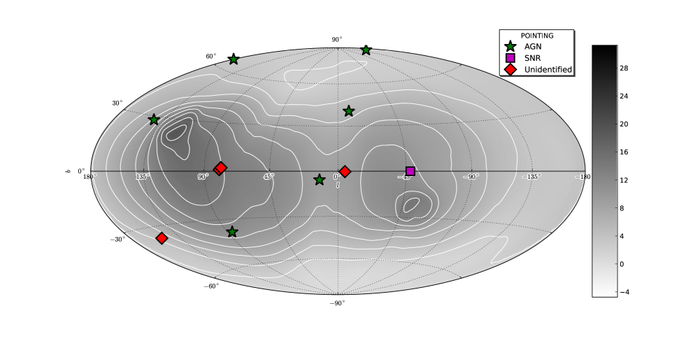
Figure 8: Position and classification of the published AGILE-GRID Astronomical Telegrams in “pointing” mode overlapped to the exposure map.

Tables 4 and 5 list the $\gamma$-ray transient sources published in Astronomical Telegrams. Figure 8 and 9 show the position and classification of the published AGILE-GRID ATels in “pointing” and “spinning” mode overlapped to the related exposure maps.

6.1 The 2010 Crab Flare Case

The Crab source (pulsar $+$ Nebula) is usually characterized by a mean flux of $F=(2.2\pm 0.1)\times 10^{-6}$ photons cm^-2 s^-1 for $E>100$ MeV at a significance of $\sqrt{T_{s}}$ = 30.0. This result is obtained with data from 2007 July to 2009 October, taking into account the diffuse $\gamma$-ray background with Galactic and isotropic components and considering all nearby sources with a fixed flux. Figure 3 shows ”the sliding lightcurve” of the 2010 September Crab Nebula flare as seen by the IASFBO SAS pipeline described in this paper.

The first alert from a source positionally consistent with the Crab was generated by the pipeline for a source intensity exceeding by 1 $\sigma$ the mean flux level (see the time segment called ”1.a” in Figure 3). An automated message was sent by e-mail and SMS on 2010 September 20, 02:04:04 UT (the yellow arrow 1.b in figure reports the alert generation). The Crab Nebula reached its maximum flux in AGILE data (see the time segment “2.a” in Figure 3) during the integration time from 2010 September 19 01:54:43 UT until 2010 September 20 23:47:51 UT. The corresponding alert was sent by e-mail and SMS on 2010 September 21 02:00:54 UT (see red arrow 2.b), about two hours after the maximum of the physical phenomena. During this period, the standard AGILE-GRID processing showed $\gamma$-ray flux levels from the Crab region of total significance above $8\,\sigma$, a highly unusual situation for two-day integrations in spinning mode. The Astronomical Telegram 2855 announcing the existence of a flaring source positionally consistent with the Crab Nebula was posted on 2010 September 22 at 14:45:00 UT Tavani et al. (2010). AGILE and Fermi-LAT produced five ATels within the short time of a few days. This procedure and alert system resulted in a very fast communication to the astrophysical community of the discovery of $\gamma$-ray variability from the Crab Nebula.

6.2 The Brightest Gamma-Ray Blazar in the Sky, 3C 454.3, the Crazy Diamond

The flat spectrum radio quasar 3C 454.3 (PKS 2251$+$158; $z$ = 0.859) is the brightest $\gamma$-ray (0.1–10 GeV) blazar detected after the launches of the AGILE and Fermi satellites. Since 2007, AGILE detected and investigated several $\gamma$-ray flares, as reported in (Vercellone et al., 2010).

The extremely rapid analysis of the AGILE $\gamma$-ray data allowed us to trigger several Target of Opportunity (ToO) observations with both ground- and space-based Observatories, such as the GLAST-AGILE Support Program (GASP; Villata et al. (2008, 2009)) of the Whole Earth Blazar Telescope (WEBT; radio, optical and infrared band); the Swift Satellite (Gehrels et al., 2004, optical, ultra-violet, soft and hard X-ray); INTEGRAL (Winkler et al., 2003, soft and hard X-ray); and MAGIC (Aleksić et al., 2012, above 100 GeV). It is of paramount importance to alert the community during the onset of a $\gamma$-ray flare (whose duration can vary from two up to several days), in order to be able to catch the peak of the $\gamma$-ray emission in a multifrequency fashion.

Such an unprecedented, panchromatic, and almost simultaneous coverage of this bright source allowed us to establish a possible correlation between the $\gamma$-ray (0.1 –10 GeV) and the optical ($R-$band) flux variations with no time delay, or with a lag of the former with respect to the latter of about half a day. Moreover, the detailed physical modeling of the spectral energy distributions when 3C 454.3 was at different flux levels provided an interpretation of the emission mechanism responsible for the radiation emitted in the $\gamma$-ray energy band, which has assumed to be inverse Compton scattering of photons from the broad-line region (BLR) clouds off the relativistic electrons in the jet, with a bulk Lorentz factor of $\Gamma\sim 20$.

On 2010 November 20, 3C 454.3 reached a peak flux ($E>$100 MeV) of $F_{\gamma}^{\rm p}=(6.8\pm 1.0)\times 10^{-5}$ ph cm^-2s^-1  on a time scale of about 12 hr, more than a factor of 6 times higher than the flux of the brightest steady $\gamma$-ray source, the Vela pulsar (Vercellone et al., 2011). The AGILE rapid alert system allowed us to follow this event and trigger several ToOs for about one month. Such a dense multifrequency coverage allowed us to detected not only the major $\gamma$-ray flare, but also a peculiar $\gamma$-ray orphan optical flare about 10 days prior to the major $\gamma$-ray flare. This puzzling behavior challenges the idea of a uniform external photon field and is still under investigation, see V. Vittorini et al. (2014, in preparation).

7 Conclusions

In this paper we described the main features of the fast $\gamma$-ray data processing of the AGILE mission. In particular, we focused on the ’spotfinder’ algorithm, the optimization of software tools, the data link from the satellite to data processing centers, the orbit-by-orbit data analysis, and the statistical characterization of the data analysis system. An important part of the data processing is the extensive use of mobile technologies coupled with the simultaneous implementation of two independent pipelines of the AGILE Alert System.

Identifying unexpected transient astrophysical events within a very short time is of crucial importance for high-energy astrophysics. The AGILE Alert System has demonstrated to be quite successful in source detection and rapid alert capability. The AGILE mission and the scientific community have certainly benefited from its implementation, which maximizes the scientific return of $\gamma$-ray observations.

Our work can be important for future high-energy astrophysics instruments operating at $\gamma$-ray energies. Very efficient data transmission to the processing center and an orbit-by-orbit data analysis are the crucial ingredients for an efficient scientific Ground Segment. The AGILE-GRID Alert System demonstrates that with a proper choice of resources, the task of automatic alerting for transient cosmic sources within two to three hours is possible. We expect this task to become an important requirement for future high-energy astrophysics instruments both in space and on the ground.

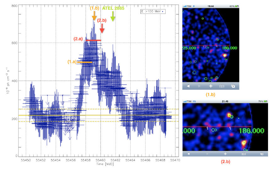
Figure 3: $96^{\prime}$ sliding light curve (with two-day integration time) of the 2010 September Crab nebula flare as seen by IASFBO SAS pipeline. Errors are $1\sigma$, and time is given in MJD. The yellow lines show the average Crab flux and the $3\sigma$ uncertainty range. 1.a and 1.b (in orange) are, respectively, the detected flux and the time of the alert generation by the IASFBO SAS pipeline when Crab nebula reaches a flux level that exceeds $1\sigma$ the mean flux level; on the right are the counts map of 1.b as seen by IASFBO SAS pipeline. 2.a and 2.b (in red) are related to the maximum flux level reached; on the right are the counts map of 2.b as seen by IASFBO SAS pipeline. The green arrow indicates the time that the Astronomical Telegram was posted.

Table 1: Performed Simulations for the Evaluation of Statistical Significance of the Blind Search Procedure for Unknown Transient Sources.

Source Position	Candidate Flares	Simulated Maps $\times 10^{6}$
Free	1	10
Free	3	5
Free	8	5
Fixed	1	8

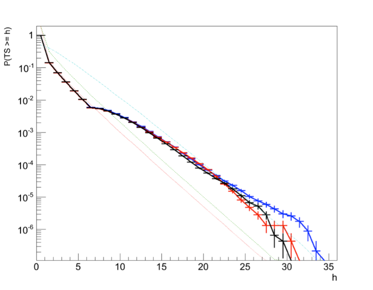
Figure 6: Histograms are the p-value distributions for an empty Galactic region when there are three sources in the ensemble of models. The blue histogram is the distribution of the first source, the red histogram is the distribution of the second source, and the black histogram is the distribution of the third source. The flux and position of the sources are left free; $g_{\rm gal}$ and $g_{\rm iso}$ parameters are free. The red dotted line is the $\frac{1}{2}\chi^{2}_{1}$ theoretical distribution, the green dashed line is the $\chi^{2}_{1}$ theoretical distribution, and the cyan dot-dashed line is the $\frac{1}{2}\chi^{2}_{3}$ distribution.

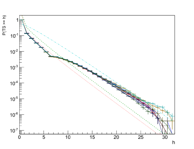
Figure 7: Histograms are the p-value distributions for an empty Galactic region when there are eight sources in the ensemble of models. The flux and position of the sources are left free; $g_{\rm gal}$ and $g_{\rm iso}$ parameters are free. The red dotted line is the $\frac{1}{2}\chi^{2}_{1}$ theoretical distribution, the green dashed line is the $\chi^{2}_{1}$ theoretical distribution, the cyan dot-dashed line is the $\frac{1}{2}\chi^{2}_{3}$ distribution.

Table 2: Fitting Results for the Parameters Reported in Equation (2) for a Different Hypothesis Formulation.

Ensemble of models	$\delta\times 10^{-4}$	$\eta_{1}\times 10^{-4}$	$\eta_{2}$
One candidate flare	$0.86\pm 2.9$	$0.45\pm 3.9$	$4.8\times 10^{-3}\pm 2.1\times 10^{-5}$
Three candidate flares - first source	$0.86\pm 4.3$	$0.45\pm 5.8$	$5.7\times 10^{-3}\pm 3.5\times 10^{-5}$
Three candidate flares - third source	$0.85\pm 4.3$	$0.46\pm 5.8$	$5.5\times 10^{-3}\pm 3.4\times 10^{-5}$
Eight candidate flares - first source	$0.85\pm 4.1$	$0.46\pm 5.6$	$4.7\times 10^{-3}\pm 3.0\times 10^{-5}$
Eight candidate flares - last source	$0.87\pm 4.1$	$0.42\pm 5.8$	$4.7\times 10^{-3}\pm 3.0\times 10^{-5}$

Table 3: Correspondence between p-value and $T_{s}$ Value for a Different Number of Point Sources in the Ensemble of Models and for Two Search Procedures Used in the IASFBO SAS pipeline.

$\sigma$ pre-trial	p-value	Fixed position		Free position
		1 candidate	1 candidate	3 candidates	8 candidates
4	$3.17\times 10^{-5}$	15.8	22.2	22.4-22.5	22.1-22.8
5	$2.86\times 10^{-7}$	24.8	33.0	33.2-33.3	32.8-33.5
6	$9.21\times 10^{-10}$	35.8	45.4	45.6-45.7	45.2-45.9

Table 4: AGILE-GRID ATels in “pointing” mode.

Positionally Consistent with	Object Class	ATels	Start (UT)	Stop (UT)	ATel ID
3C 454.3	Blazar	8	2007 Jul 24 14:30	2007 Jul 27 05:27	1160
			2007 Jul 24 14:30	2007 Jul 30 11:40	1167
			2007 Nov 02 13:50	2007 Nov 12 17:01	1278
			2007 Nov 02 12:00	2007 Nov 22 18:33	1300
			2008 May 24 03:10	2008 May 27 04:17	1545
			2008 Jun 15 10:46	2008 Jun 16 07:11	1581
			2008 Jun 25 03:00	2008 Jun 26 03:00	1592
			2008 Jul 25 18:00	2008 Jul 28 03:00	1634
PKS 1510-089	Blazar	4	2008 Mar 18 03:00	2008 Mar 20 03:00	1436
			2009 Mar 08 14:00	2009 Mar 10 4:00	1957
			2009 Mar 12 07:00	2009 Mar 13 05:00	1968
			2009 Mar 18 05:45	2009 Mar 19 05:33	1976
PKS 1830-211	Blazar	1	2009 Oct 12 00:03	2009 Oct 13 04:57	2242
Mkn 421	Blazar	1	2008 Jun 09 17:02	2008 Jun 15 02:17	1583
3EG J0721+7120	Blazar	1	2007 Sep 10 13:50	2007 Sep 20 10:13	1221
3EG J1410-6147	SNR	1	2008 Feb 21 06:00	2008 Feb 22 07:30	1394
W Comae	Blazar	1	2008 Jun 09 17:02	2008 Jun 15 02:17	1582
AGLJ2021+4029	Unidentified	3	2008 Apr 27 01:39	2008 Apr 28 01:27	1492
			2008 May 22 06:00	2008 May 27 06:00	1547
			2007 Nov 02 12:00	2008 May 01 00:00	1585
AGL J2021+4032	Unidentified	1	2008 Nov 16 14:33	2008 Nov 17 14:22	1848
AGL J2030+4043	Unidentified	1	2008 Nov 02 20:43	2008 Nov 03 20:32	1827
AGL J0229+2054	Unidentified	1	2008 Jul 30 15:34	2008 Jul 31 15:23	1641
AGL J1734- 3310	Unidentified	1	2009 Apr 14 00:00	2009 Apr 15 00:00	2017

Table 5: AGILE-GRID ATels in “spinning” mode.

Positionally Consistent with	Object Class	ATels	Start (UT)	Stop (UT)	ATel ID
3C 454.3	Blazar	6	2009 Nov 26 01:00	2009 Dec 2 08:30	2322
			2009 Dec 2 06:30	2009 Dec 3 08:30	2326
			2010 Oct 28 06:00	2010 Oct 31 06:00	2995
			2010 Nov 16 06:50	2010 Nov 17 09:15	3034
			2010 Nov 18 03:15	2010 Nov 19 09:15	3043
			2010 Nov 21 04:50	2010 Nov 22 04:50	3049
PKS 1510-089	Blazar	5	2010 Jan 11 10:30	2010 Jan 13 10:30	2385
			2011 Jul 2 04:30	2011 Jul 4 04:30	3470
			2012 Jan 28 12:00	2012 Feb 1 12:00	3907
			2012 Feb 14 04:00	2012 Feb 17 04:30	3934
			2013 Sep 22 12:00	2013 Sep 24 12:00	5422
PKS 1830-211	Blazar	2	2009 Nov 20 17:00	2009 Nov 22 17:00	2310
			2010 Oct 15 00:00	2010 Oct 17 00:00	2950
PKS 0402-362	Blazar	2	2010 Mar 13 12:00	2010 Mar 16 15:00	2484
			2011 Aug 8 04:10	2011 Aug 10 09:04	3544
PKS 1222+216	Blazar	3	2009 Dec 13 06:00	2009 Dec 15 06:00	2348
			2010 May 23 14:30	2010 May 26 05:22	2641
			2010 Jun 17 09:20	2010 Jun 19 09:30	2686
BL Lac	Blazar	1	2011 May 27 11:57	2011 May 29 11:30	3387
S41749+70	Blazar	1	2011 Feb 26 00:00	2011 Mar 1 04:00	3199
4C +3841	Blazar	2	2012 Sep 15 22:00	2012 Sep 18 10:30	4389
			2013 Jul 25 06:00	2013 Jul 27 15:00	5234
2FGL J1823.8+4312	Blazar	1	2012 Jun 3 04:00	2012 Jun 5 04:00	4153
2FGL J1127.6+3622	Blazar	1	2011 Nov 17 00:00	2010 Nov 19 00:00	3858
PKS J2329-4955	Blazar	1	2010 Nov 1 00:00	2010 Nov 5 03:00	3008
PKS 1830-211	Blazar	1	2010 Oct 15 00:00	2010 Oct 17 00:00	2950
PKS 2142-758	Blazar	1	2010 Apr 10 11:30	2010 Apr 12 21:00	2551
PKS 0537-441	Blazar	1	2010 Feb 18 00:00	2010 Feb 23 10:30	2454
3C 273	Blazar	1	2010 Jan 6 16:50	2010 Jan 8 07:50	2376
PKS 2233-148	Blazar	1	2012 Jun 3 10:00	2012 Jun 5 22:00	4154
PMN J0948+0022	Seyfert 1	1	2011 Jun 20 07:30	2011 Jun 22 11:20	3448
Cygnus X-1	Binary	2	2010 Mar 24 02:24	2010 Mar 25 01:01	2512
			2010 Jun 30 10:00	2010 Jul 2 10:00	2715
Cygnus X-3	Binary	6	2010 May 7 14:53	2010 May 9 17:19	2609
			2010 May 25 19:10	2010 May 27 17:04	2645
			2011 Jan 27 20:00	2011 Feb 1 11:00	3141
			2011 Feb 6 05:00	2011 Feb 8 09:00	3151
			2011 Mar 20 00:00	2011 Mar 20 00:00	3239
			2011 May 28 07:58	2011 May 29 06:02	3386
PSR B1259-63	Pulsar	1	2010 Aug 2 06:400	2010 Aug 4 04:00	2772
Crab Nebula	SNR	6	2010 Sep 19 00:10	2010 Sep 21 00:10	2855
			2011 Apr 9 23:45	2011 Apr 13 23:45	3282
			2011 Apr 15 10:40	2011 Apr 16 10:38	3286
			2013 Mar 3 05:30	2013 Mar 4 11:00	4856
			2013 Mar 5 13:00	2013 Mar 6 13:00	4867
			2013 Oct 18 00:00	2013 Oct 19 00:00	5506
AGL J1647+5107	Unidentified	1	2013 Feb 22 15:00	2013 Feb 24 17:18	4842
AGL J2302-3251	Unidentified	1	2011 May 14 03:00	2011 May 17 03:00	3357
AGL J2241+4454	Unidentified	1	2010 Jul 25 01:00	2010 Jul 26 23:30	2761
AGL J0906-1241	Unidentified	1	2010 Apr 11 05:00	2010 Apr 13 06:00	2552
AGL J0109+6134	Unidentified	1	2010 Jan 31 08:20	2010 Feb 2 19:48	2416
AGL J2206+6203	Unidentified	1	2010 Jan 20 03:46	2010 Jan 25 11:15	2403
AGL J1023-3738	Unidentified	1	2009 Dec 25 22:30	2009 Dec 27 22:10	2361
MAXI J1659-152	Unidentified	1	2010 Sep 25 00:00	2010 Sep 26 14:00	2880
AGL J0813+2420	Unidentified	1	2010 Oct 23 18:00	2010 Oct 26 06:00	2971
AGL J1037-5708	Unidentified	1	2010 Nov 27 21:18	2010 Nov 30 14:08	3059
AGL J2103+5630	Unidentified	1	2011 Aug 8 04:10	2011 Aug 10 09:04	3544
AGL J1524+3642	Unidentified	1	2012 Jan 9 11:26	2012 Jan 11 10:57	3862

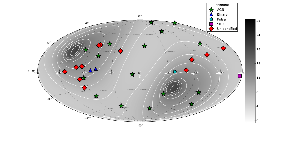
Figure 9: Position and classification of the published AGILE-GRID Astronomical Telegrams in “spinning” mode overlapped to the exposure map.

References

- Abdo et al. (2009) Abdo, A.A., Ackermann, M., Ajello, M., et al., 2009a, APh, 32, 193
- (2) Abdo, A.A., Ackermann, M., Ajello, M., et al., 2009b, Sci, 326, 1512
- Ackermann et al. (2013) Ackermann, M., Ajello, M., Albert, A., et al., 2013, ApJ, 771, 57
- Aleksić et al. (2012) Aleksić, J., Alvarez, E. A., Antonelli, L. A., et al. 2012, APh, 35, 435
- Atwood et al. (2009) Atwood, W. B., Abdo, A. A., Ackermann, M., et al. 2009, ApJ, 697, 1071
- Buehler et al. (2010) Buehler, R., D’Ammando, F., & Hays, E. 2010, ATel, 2861
- (7) Bulgarelli, A., Tavani, M., Chen, A. W., et al., 2012a, AA , 538, A63
- (8) Bulgarelli, A., Chen, A. W., Tavani, M., et al., 2012b, AA , 540, A79
- Chen et al. (2013) Chen, A. W., Argan, A., Bulgarelli, A., et al, 2013, AA , 558, A37
- Di Stefano & Bulgarelli (1999) Di Stefano, L., & Bulgarelli, A. 1999, Proc. of 10th International Conference on Image Analysis and Processing, doi: 10.1109/ICIAP.1999.797615
- Fichtel & Trombka (1997) Fichtel, C.E., & Trombka, J.I., 1997, Gamma-Ray Astrophysics, NASA Reference Publication 1386
- Gehrels et al. (2004) Gehrels, N., Chincarini, G., Giommi, P., et al. 2004, ApJ, 611, 1005
- Giuliani et al. (2004) Giuliani, A., Chen, A., Mereghetti, S., et al., 2004, MSAIS, 5, 135
- Hartman et al. (1999) Hartman, R. C., Bertsch, D. L., Bloom, S. D., et al., 1999, ApJS, 123, 79
- Hinton & Starling (2013) Hinton, J. A., & Starling, R. L. C. 2013, Phil. Trans. R. Soc., 371, 1992
- Mayer-Hasselwander (1979) Mayer-Hasselwander, H.A., 1979, in Annals of the New York Academy of Sciences, Proc. of the Ninth Texas Symposium, 226, 211
- Nolan et al. (2012) Nolan, P. L., Abdo, A. A., Ackermann, M., et al., 2012, ApJS, 199, 31
- Piano et al. (2012) Piano, G., Tavani, M., Vittorini, V., et al. 2012, AA , 545, A110
- Pittori et al. (2009) Pittori, C., Verrecchia, F., Chen, A. W., et al. 2009, AA , 506, 1563
- Pittori et al. (2013) Pittori, C., et al. 2013, Nuclear Physics B (Proc. Suppl.), vol. 239, 104
- Rosenfield & Pfaltz (1966) Rosenfield, A., & Pfaltz, J., 1966, J. ACM, 13, 471
- Swanenburg et al. (1981) Swanenburg, B.N., Bennett, K., Bignami, G. F., et al., 1981, ApJL, 242, L69
- Tavani et al. (2008) Tavani, M. ,Sabatini, S., Piano, G., et al., 2008, ATel, 1827
- (24) Tavani, M., Barbiellini, G., Argan, A., et al. 2009a, AA , 502, 995
- (25) Tavani, M., Bulgarelli, A., Piano, G., et al. 2009b, Natur, 462, 620
- Tavani et al. (2010) Tavani, M., Striani, E., Bulgarelli, A., et al., 2010, ATel, 2855
- Tavani et al. (2011) Tavani, M., Bulgarelli, A., Vittorini, V., et al. 2011, Sci, 331, 736
- Thompson et al. (1993) Thompson, D.J., Bertsch, D. L., Fichtel, C. E., et al., 1993, ApJS, 86, 629
- Trifoglio et al. (2007) Trifoglio, M., et al., 2013, arXiv:1305.5389
- Trifoglio et al. (2008) Trifoglio, M., Bulgarelli, A., Gianotti, F., et al. 2008, Proc. SPIE, 7011, 70113E
- Vercellone et al. (2010) Vercellone, S., D’Ammando, F., Vittorini, V., et al. 2010, ApJ, 712, 405
- Vercellone et al. (2011) Vercellone, S., Striani, E., Vittorini, V., et al., 2011, ApJL, 736, L38
- Villata et al. (2009) Villata, M., Raiteri, C. M., Gurwell, M. A., et al. 2009, A&A, 504, L9
- Villata et al. (2008) Villata, M., Raiteri, C. M., Larionov, V. M., et al. 2008, A&A, 481, L79
- Winkler et al. (2003) Winkler, C., Courvoisier, T. J.-L., Di Cocco, G., et al. 2003, A&A, 411, L1-L6