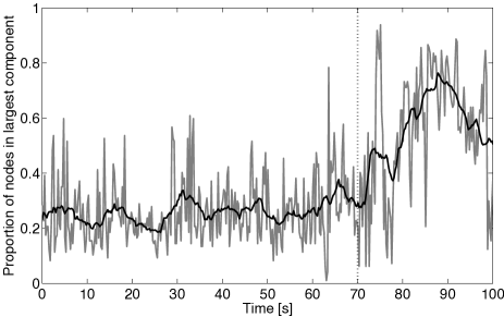
[2]footnote ††thanks: The authors marked have equally contributed to the production of this article. CEG is the corresponding author. ††thanks: EDK and CEG were supported by a grant from the Air Force Office for Scientific Research (AFOSR), whose grant number is FA9550-12-1-0102. MAK was supported by a Career Award at the Scientific Interface from the Burroughs Wellcome Fund. The authors thank Dr. Sydney Cash for providing the brain voltage data analyzed in Figure 1.
Percolation under Noise:
Detecting Explosive Percolation Using the Second Largest Component
Abstract
We consider the problem of distinguishing classical (Erdős-Rényi) percolation from explosive (Achlioptas) percolation, under noise. A statistical model of percolation is constructed allowing for the birth and death of edges as well as the presence of noise in the observations. This graph-valued stochastic process is composed of a latent and an observed non-stationary process, where the observed graph process is corrupted by Type I and Type II errors. This produces a hidden Markov graph model. We show that for certain choices of parameters controlling the noise, the classical (ER) percolation is visually indistinguishable from the explosive (Achlioptas) percolation model. In this setting, we compare two different criteria for discriminating between these two percolation models, based on a quantile difference (QD) of the first component’s size and on the maximal size of the second largest component. We show through data simulations that this second criterion outperforms the QD of the first component’s size, in terms of discriminatory power. The maximal size of the second component therefore provides a useful statistic for distinguishing between the ER and Achlioptas models of percolation, under physically motivated conditions for the birth and death of edges, and under noise. The potential application of the proposed criteria for percolation detection in clinical neuroscience is also discussed.
I Introduction
Understanding the emergence of organized structure in dynamic networks remains an active research area. In the study of random networks, percolation –the sudden emergence of a giant connected component (GCC)– is of critical importance from a theoretical, applied and statistical perspective. Percolation in the Erdős-Rényi (ER) model constitutes one of the first examples of a fully characterized mathematical phase transition (Erdős and Rényi, 1960; Alon and Spencer, 2004). While the ER model of percolation is an example of a (second order) continuous phase transition, recent efforts have focused on identifying the conditions under which a random network process can yield a (first order) discontinuous percolation (Riordan and Warnke, 2011).
One of most popular attempts to model discontinuous percolation has been the Achlioptas’ process and its variants (Achlioptas et al., 2009). The Achlioptas’ product rule (PR) slows down the growth of the GCC by favoring the creation of edges between small connected components. Although this particular percolation model has been shown to be, in fact, continuous and therefore of second order (Riordan and Warnke, 2011, 2012); it nonetheless provides an interesting alternative to the ER model. Achlioptas’ processes have indeed generated a substantial amount of theoretical work, whereby authors have explored related strategies for producing explosive percolation in random networks (Bohman and Frieze, 2001; Beveridge et al., 2007; Krivelevich et al., 2010). In addition, Riordan and Warnke (2011) have shown that genuine first-order phase transitions can be realized by systematically adding, at every step of the process, the edge that joins the two smallest components in the entire network.
Interest in network percolation has been fueled by its relevance to several application domains. In clinical neuroscience, for instance, epileptic seizures have been associated with the sudden emergence of coupled activity across the brain (Guye et al., 2006; Ponten et al., 2007; Schindler et al., 2007b, a; Kramer et al., 2010; Schindler et al., 2010). The resulting functional networks –in which edges indicate strong enough coupling between brain regions (Rubinov and Sporns, 2010)– are consistent with the notion of percolation. A better understanding of the type of phase transitions undergone at different stages of the seizure, may aid in the development of novel strategies for the treatment of epilepsy (Kramer and Cash, 2012).
The rich theory on percolation, and its application to real world data, motivates the following question: How can we distinguish between different percolation regimes in practice? Previous theoretical work has concentrated on noise-free percolation, which constitutes an idealized perspective on percolation processes. In practice, however, the sampling of real-world networks is likely to be corrupted by measurement errors. Moreover, network growth has generally been conceived as a monotonic process, whereby only edge creations are allowed. However, this assumption may be too restrictive, since in real-world networks, the number of edges may increase and decrease over time, in a stochastic manner (see example in Figure 1). Finally, to the best of our knowledge, there does not currently exist a statistical framework for distinguishing between different types of percolation regimes in the presence of edge birth and death, and noise.
In this paper, we propose a framework to distinguish between different percolation regimes in practice. To do so, we formulate the problem of recognizing a percolation regime from noisy observations as a question of statistical inference. Under this framework, we compare the discriminatory power of two potential percolation features deduced from the evolution of the first and second component of an observed dynamic network. We test this framework in simulation by constructing a hidden Markov graph model, which encompasses both a non-stationary latent process characterized by birth and death of edges, and an observed graph process that introduces both Type I and Type II errors. We show that edge death and noise make a statistic deduced from the first component ineffective in distinguishing between the standard ER second-order percolation and Achlioptas’ explosive percolation. However, a different detection criterion –based on the size of the second component– successfully discriminates between the two percolation regimes in the presence of edge death and noise. These results provide a framework for distinguishing percolation regimes in practice.
II Percolation Models
II.1 Birth/Death Erdős-Rényi (ER) Process
We first construct a graph-valued stochastic process that exhibits the Markov property. This provides a realistic model for generating noisy percolation processes, while maintaining a sufficient level of computational tractability. We will denote a sequence of graph-valued random variables on vertices by
| (1) |
At each time step, a single edge is either added or deleted. Such a sequence will be said to be Markov if its edge sets are controlled by a Markov chain. We impose this dependence through the use of a binary random variable, denoted , whose state space is . This Markov chain is characterized by the following transition probability matrix , for some choices of the birth and death rates, denoted respectively by and , and taking values in .
Following customary notation, the entries of will be denoted by , with rows summing to one. The graph-valued Markov chain, , is then obtained by associating with the addition or deletion of an edge in each edge set, . Thus, provided that , it follows that the state space of this graph-valued Markov chain is the space of all simple graphs on vertices, since every graph is reachable with positive probability.
In general, and are not required to sum to one. It will be of interest to let in order to study the large-scale behavior of the ’s as the graph process accumulates edges. Moreover, observe that is a (time) homogeneous Markov chain, since , for any and every .
Now, suppose that there exist edges at time in and let denotes the ‘status’ of edge at time , such that , if that edge is present and , otherwise. Note that we have here two different sources of dependence. On one hand, the edges are dependent on each other, since no more than one edge can be added or deleted at every time step. On the other hand, the edges are also dependent over time, since the status of an edge at time depends on the status of that same edge at time .
In the sequel, we will concentrate on a special case of this birth and death process, where we will set . This leads to simplified marginal distributions for the edges. Additional details of this birth and death model are provided in appendix A.
II.2 Birth/Death Product Rule (PR) Process
We extend the standard Achlioptas’ framework of PR percolation to a birth and death process, by devising death steps. This model is analogous to the aforementioned ER birth/death model, except for the choice of the probability distribution of the latent ’s. As for the ER birth/death model, a binary random variable, , controls the addition or deletion of edges in each . However, in the case of the PR model, the choice of the edge to be added or to be deleted is not uniform over the ’s. Here, this choice depends on the modular structure of the graph at time . Therefore, as for the ER model, we obtain a non-stationary stochastic process.
Assuming that , the addition of a new edge is conducted by uniformly choosing two candidate vertex pairs among all the edges in , the complement of the edge set, . These two candidate edge pairs are denoted by and , and satisfy and , since , as in Figure 2. We then evaluate the size of the connected components to which , , and belong. These four connected components are denoted by , , , and , respectively. Then, following Achlioptas et al. (2009), we apply the following product rule: If , then ; otherwise, .
Conversely, the death or deletion of an edge is handled in a symmetric manner. When , we uniformly select two candidate edges from . These vertex pairs are denoted and and satisfy and , since . Next, we set and , in order to compute the size of the connected components to which , , and would belong to, if these edges were absent. This is done in order to ensure that the deletion of an edge exactly corresponds to the reverse operation of the addition of an edge under PR. Now, after having deleted these edges and computed the sizes of , , , and ; we decide which edge should re-enter , in order to produce . Such a decision is also based on the PR, such that if , then ; otherwise, .
This choice of specification for the death step ensures that the ordering of the creation and deletion of edges are symmetrical. Given a sequence of two edges successively born during two time steps of , if we encounter a death step, where both and are selected, we would then delete these edges in the reverse order, by eliminating before . This order-preserving property is illustrated in Figure 2. This constraint ensures that births and deaths are genuine reverse PR operations. In addition, observe that, as for the ER percolation process, this chain is irreducible, in the sense that there is positive probability of transitioning from any given edge configuration to any other in the space of the edge sets of .
II.3 Hidden Markov Graph Model
Next, we assume that there exists a time-independent error process, which produces at each time point an observed edge status . This stochastic process is governed by two additional parameters and , whose behavior can be described using a traditional ‘confusion matrix’, such that for any , we have
The ’s and ’s are here treated as latent and observed stochastic processes, respectively, and and can therefore be interpreted as the Type I (false positive) and Type II (false negative) error probabilities. Combining the graph-valued Markov latent process with this time-independent error process, we obtain a graph-valued hidden Markov process, as described in figure 3. From this schematic representation, one can immediately see that the observed graphs denoted , and are conditionally independent, given the latent graph process, .
For the ER model, under the assumption that , these two stochastic graph processes can be combined by taking into account the time-dependence of the ’s. In this case, the corresponding transition matrix linking the observed and latent processes is available in closed-form. Details of these derivations are provided in appendix A.
III Detecting Explosive Percolation
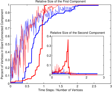
Explosive percolation is expected to produce a sharper phase transition than a typical ER percolation. When considering noisy observations, however, detecting such differences through visual inspection only is hard. Figure 4 illustrates this problem, by comparing noisy and noise-free graph sequences for both explosive and ER models. Beyond visual inspection, the problem of discriminating between these two models of percolation can be formulated as a hypothesis-testing problem: The null hypothesis, denoted , states that the observed process corresponds to an ER percolation, whereas the alternative hypothesis, , is that the observed process does not correspond to this type of percolation model.
To proceed with this hypothesis-testing problem in practice, we specify a population parameter summarizing the percolation process, say and , for the ER and target models, respectively. This leads to a hypothesis test of the form,
Several population parameters could be used for the purpose of discriminating between these two models of percolation. A natural candidate for such parameters would be a measure of the sharpness of the transition of the first component’s size. The main panel of Figure 4, however, suggests that this population parameter will not have sufficient discriminatory power, when confronted with a substantial amount of observational noise.
Therefore, as a second candidate population parameter, we consider the following natural extension: The size of the second largest component. This appears to provide a more sensitive marker of the sharp phase transition exhibited by explosive percolation models. This ‘second-order’ property is motivated by the mechanism of the product rule, which underlies the Achlioptas’ graph process, which we will use as representative of the alternative hypothesis, (i.e., reducing our testing problem to the comparison of two point null hypotheses). In what follows, we will show that the use of the size of the second largest component as a statistical marker to distinguish the two percolation regimes exhibits greater discriminatory power, than a statistic solely based on the first component.
The differences between the candidate percolation models are therefore quantified using two criteria: (i) a quantile difference (QD) of the distribution of the size of the GCC, and (ii) the maximal size of the second component over the entire time period. These two criteria are formally defined as follows. Given the graph process, , and denoting the vertex subset of the largest component in by , we define the cumulative edge function as the cardinality of , normalized by the maximal number of edges in the graph, such that
Although this function is not a cumulative distribution function (CDF), one can nonetheless uniquely define quantiles using the standard definition of quantiles for the CDFs of discrete random variables; such that for any , we have
where is the maximal number of time steps in the graph process. In this paper, we are especially interested in quantile differences of the following form, which can be treated as a generalization of the classical interquartile range,
One can observe from Figure 1 that the size of the GCC, in the functional networks associated with a seizure, rarely exceeds 80. Therefore, we have here adopted a quantile difference that reflects the range of the distribution of the GCC in this practical setting. Thus, the criterion of interest will be the following, . This parameter quantifies the steepness of the phase transition, the larger the QD criterion, the longer the transition to a fully connected graph.
As a second criteria to distinguish the two percolation regimes, we consider the maximal size attained by the second largest component over the entire time period of the dynamic network observation. If one defines the vertex set of the second largest component at time by , this second criterion can be expressed as . This quantity is expected to constitute a good marker of the steepness of the phase transition, since it reflects the extent of separation of the graph process into large connected subgraphs. Indeed, a direct consequence of the Achlioptas’ construction rule is that by inhibiting the growth of a single large component, we necessarily increase the production of several subcomponents.
Statistical inference on these two criteria is then drawn using a Monte Carlo hypothesis test. Letting the parameter , and selecting the candidate percolation to be drawn from a PR process, we consider the following null and alternative hypotheses,
respectively. The direction of this test is justified by the fact that we expect explosive percolation to occur rapidly, and thus to exhibit a smaller amount of variability in the size of its GCC, when transitioning to a fully connected graph. Our second criterion, by contrast, is tested in the opposite direction, since we naturally anticipate the PR process to be characterized by a larger maximal second component. Thus, for , the alternative hypothesis becomes .
(a)
(b)
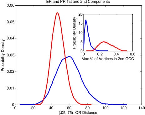
In the results reported in this paper, the distributions of the ER and PR graph processes are known. It therefore suffices to simulate from these densities in order to construct the distribution of the two test statistics at hand. This procedure is illustrated in figure 5. We are especially interested in the discriminatory powers of these statistics, and we will therefore compare their respective merits, using the true positive and false positive rates, within a receiver operating characteristic (ROC) framework. For presentational convenience, the distributions of interest were smoothed using a normal density kernel, before computing the ROC curves and corresponding areas under the curves (AUCs). The computation of the AUCs allows us to summarize the differences between the models over the entire time period.
IV Results
IV.1 Birth/Death Processes
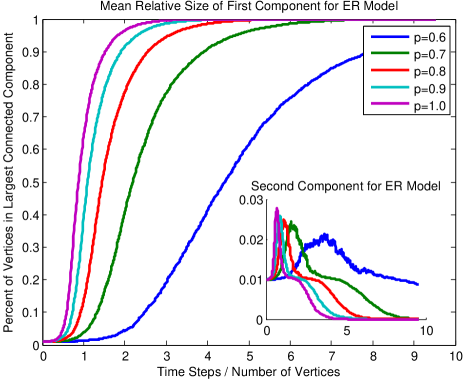
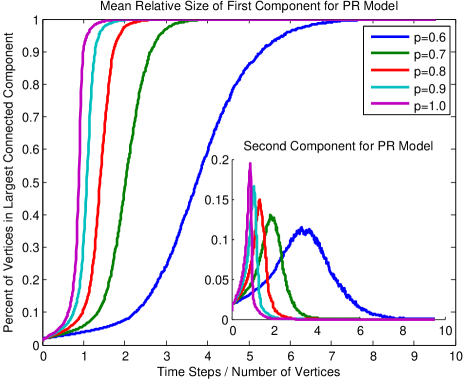
The ER and PR percolation models were simulated on graphs of vertices. We first explored the effect of varying the birth and death rates on the behavior of the two statistical criteria of interest, under the ER and PR models. The results of these Monte Carlo simulations are reported in Figure 6, where each curve is the mean of 1,000 different synthetic data sets. In these simulations, the death rate was set to , and therefore the value of controls both the birth and death rates.
The main effect of a change in is to delay percolation, and to diminish the steepness of the phase transition. Observe that as decreases, percolation tends to occur at a later time step in both the ER and PR models (Figure 6). In particular, for the lowest birth rate that we investigated , the ER model did not produce a fully connected graph within the number of iterations considered, as can be seen from Figure 6(a). When was set to values equal to or less than , no phase transition could be observed, and these results are not reported.
The size of the second component was similarly affected by changes in . Decreasing the birth rate delayed the time at which the size of the second component attained its highest value. Moreover, lower values of also yielded second components with smaller maximal sizes, under both the ER and PR models. Interestingly, we note that the time points at which the second components reach a maximal size tend to coincide in both models. Thus, it would be difficult to distinguish between these two percolation models on the sole basis of the timing of the occurrence of the maximal size of the second components. By contrast, the relative maximal size of the second components in the ER and PR models differ by approximately one order of magnitude, thereby providing a natural criterion for discriminating between these two types of percolation, as can be observed by comparing the inset figures in 6(a) and 6(b).
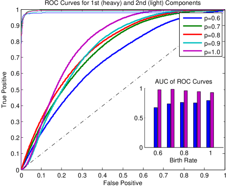
We formally quantified these differences in discriminatory powers by studying the ROC curves of these two criteria under different choices of (Figure 7). The maximal size of the second component substantially outperforms the relative size of the first component, for all values of . The stark difference between these discriminatory criteria can be understood by considering the amount of overlap of the distributions of these two criteria in Figure 5. Whereas the distributions of the QD of the size of the GCC under the two models exhibit a large amount of overlap; the distributions of the maximal size of the second component, by contrast, share very little common support. These differences in support account for the substantive gains in discriminatory power by the maximal size of the second component, reported in Figure 7.
In addition, we note the QD of the size of the first component was more sensitive to choices of than the maximal size of the second component. As diminishes, it becomes increasingly more difficult to discriminate between the ER and PR percolation models, using the QD of the size of the first component. This suggests that this criterion is more sensitive to a non-zero death rate, than the maximal size of the second component, which provides further support for the use of this latter criterion, in practice.
(a)
(b)
IV.2 Percolation under Noise
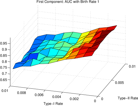
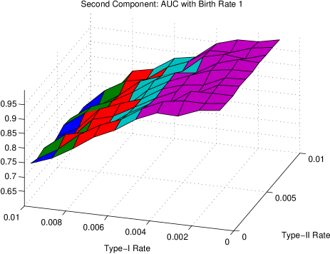
Secondly, we considered the effect of introducing noise in these models. The results reported in Figure 8 were produced using our proposed hidden Markov graph model, and are averaged over 1,000 simulations. We were especially interested in the effect of Type I and Type II errors on our ability to discriminate between classical and explosive percolation, using the two criteria under scrutiny. Both the Type I and Type II error rates were made to vary between and .
From Figure 8, one can observe that the two types of errors had markedly different effects on the AUCs of the two discriminatory criteria. Introducing Type I errors led to a substantial diminution of the AUCs for both the QD of the size of the first component in (a), and the maximal size of the second component in (b). In particular, note that the two criteria reached equivalent levels of discriminatory power for . Thus, although the maximal size of the second component remains a more useful criterion for distinguishing between the ER and PR models than the QD of the size of the first component, these two criteria exhibit comparable performance, under a moderate amount of Type I error.
The impact of increasing the Type II error rate on the behavior of these two criteria was negligible. Introducing false negatives in the ER and PR models slightly increased the AUCs of both the QD of the first component’s size, and the maximal size of the second component. Thus, large Type II error rates may be marginally advantageous for discriminating between these two models of percolation, under the scenarios studied.
V Discussion and Conclusions
In this paper, we have extended existing models of percolation, by allowing for edge deletion steps and noisy observations. These modeling extensions have been articulated within a hidden Markov graph process, which builds links with the existing literature on the statistical properties of this family of models (Flocchini et al., 2012; Casteigts et al., 2012; Lentz et al., 2013). Moreover, we have compared different summary statistics for distinguishing between the ER and PR percolation models. Overall, for different birth and death rates, and for a range of noise levels, the maximal size of the second component was found to have greater discriminatory power than the QD of the size of the GCC.
Several methodological challenges remain before such models can be directly used for percolation detection on real-world data. Throughout this paper, we have considered the QD of the size of the first component, using a particular choice of quantiles for this discriminatory criterion. In practice, an optimal choice of quantiles for quantifying the steepness of such phase transitions may be motivated by different factors, including (i) the range of the observations, and (ii) the need for early detection. We discuss these two practical aspects, in turn.
Firstly, note that when considering real-world applications, we rarely observe fully connected networks. In the data reported in Figure 1, for instance, the size of the GCC encompasses at most 90% of the edges in the saturated network. The choice of the quantile interval of interest for the first component will be therefore automatically constrained by the range of the observations in the data at hand. Therefore, as in sequential detection analysis, the statistical objective is to detect the outcome, on the basis of as little data as possible. Such constraints would naturally lead to a relatively narrow quantile range.
Secondly, in the context of clinical neuroscience and with particular emphasis on the prevention of a seizure; the detection of a percolation regime may be linked with patients’ health and survival. In such cases, early detection will usually be favored, as this is likely to be associated with desirable clinical outcomes. Explosive percolation, such as the Achlioptas’ PR process studied in this paper, is consistent with the sudden manifestation of a seizure as a highly synchronized event. Classifying models of percolation may then be utilized to deepen understanding of seizures in epilepsy, and a statistical identification of explosive phase transitions may facilitate immediate, targeted intervention (e.g., an electrical stimulus).
Further work in this area could be focused on estimating a percolation model from a given sequence of observed networks. In this sense, this work also contributes to the growing literature on time-indexed graph processes (Grindrod and Higham, 2009). In such cases, the birth and death rates will need to be estimated, as well as the Type I and Type II error probabilities. These different parameters may not be fully identifiable from the data, and further constraints are likely to be necessary, in order to discriminate between the two percolation models considered in this paper. Such estimation, however, may be amenable to a Bayesian formulation, as commonly implemented for hidden Markov models (Ephraim and Merhav, 2002).
Appendix A Details of Birth/Death ER Process
Here, we describe the closed-form formulas of the probabilities of edge inclusion and edge deletion in the observed graph processes under the ER model. These analytic results are obtained by assuming that the birth and death probabilities are straightforwardly related, such that . Such derivations may be useful for other authors, who may want to replicate these results, or extend the applications of the noisy model of percolation.
In this birth and death graph process, each edge is treated separately by integrating out the dependence of all other edges in the graph, and considering the marginal distribution of every . As before, we will here refer to as the latent edge status, and will indicate the number of edges in the graph at time . Given the Markov random variable , the conditional transition matrix for every , given some value of takes the following form,
where denotes the number of edges in a saturated graph of size , and where is the indicator function, which takes a value of if is true and 0, otherwise.
In this paper, we have concentrated on a special case of this birth/death process, where we have set . This choice of and leads to the following characterization of the process,
| (2) | ||||
and similarly, . Under this simplifying assumption, the preceding conditional transition matrix becomes
Each entry is obtained by taking the expectation with respect to . That is, , for every , and where the marginal distribution of is known from equation (2).
One can now combine the noise process described in section II.3, with the birth and death stochastic process in order to link the latent and observed parts of the Markov hidden model. This gives the following table,
Since this transition matrix links the latent and observed stochastic processes, one can immediately derive the marginal probabilities of the ’s, such that
and similarly for .
The resulting process is non-stationary. Moreover, this also holds when considering the case . Indeed, since the probability of adding a new edge at time is dependent on the number of existing edges, , at time ; it follows that the resulting joint distribution of any subset of the ’s depends on the choice of .
References
- Achlioptas et al. (2009) Achlioptas, D., D’Souza, R.M., and Spencer, J. (2009). Explosive percolation in random networks. Science, 323(5920), 1453–1455.
- Alon and Spencer (2004) Alon, N. and Spencer, J. (2004). The Probabilistic Method. Springer, London.
- Beveridge et al. (2007) Beveridge, A., Bohman, T., Frieze, A., and Pikhurko, O. (2007). Product rule wins a competitive game. Proc. Amer. Math. Soc, 135, 3061–3071.
- Bohman and Frieze (2001) Bohman, T. and Frieze, A. (2001). Avoiding a giant component. Random Structures and Algorithms, 19, 75.
- Casteigts et al. (2012) Casteigts, A., Flocchini, P., Quattrociocchi, W., and Santoro, N. (2012). Time-varying graphs and dynamic networks. International Journal of Parallel, Emergent and Distributed Systems, 27(5), 387–408.
- Ephraim and Merhav (2002) Ephraim, Y. and Merhav, N. (2002). Hidden markov processes. IEEE Transactions on Information Theory, 48(6), 1518–1569.
- Erdős and Rényi (1960) Erdős, P. and Rényi, A. (1960). The evolution of random graphs. Publ. Math. Inst. Hungar. Acad. Sci., 5, 17.
- Flocchini et al. (2012) Flocchini, P., Mans, B., and Santoro, N. (2012). On the exploration of time-varying networks. Theoretical Computer Science, 469, 53–68.
- Grindrod and Higham (2009) Grindrod, P. and Higham, D. (2009). Evolving graphs: Dynamical models, inverse problems and propagation. Proceedings of the Royal Society, Series A, 0456, 1–18.
- Guye et al. (2006) Guye, M., Regis, J., Tamura, M., Wendling, F., Gonigal, A.M., Chauvel, P., and Bartolomei, F. (2006). The role of corticothalamic coupling in human temporal lobe epilepsy. Brain, 129(7), 1917–1928.
- Kramer et al. (2010) Kramer, M., Eden, U., Kolaczyk, E., Zepeda, R., Eskandar, E., and Cash, S. (2010). Coalescence and fragmentation of cortical networks during focal seizures. Journal of Neuroscience, 30, 10076–10085.
- Kramer et al. (2009) Kramer, M., Eden, U., Cash, S., and Kolaczyk, E. (2009). Network inference with confidence from multivariate time series. Phys. Rev. E., 79, 061916.
- Kramer and Cash (2012) Kramer, M.A. and Cash, S.S. (2012). Epilepsy as a disorder of cortical network organization. The Neuroscientist, 18(4), 360–372.
- Krivelevich et al. (2010) Krivelevich, M., Lubetzky, E., and Sudakov, B. (2010). Hamiltonicity thresholds in Achlioptas processes. Random Struct. Alg., 37(1), 1–24.
- Lentz et al. (2013) Lentz, H.H.K., Selhorst, T., and Sokolov, I.M. (2013). Unfolding accessibility provides a macroscopic approach to temporal networks. Phys. Rev. Lett., 110(11), 118701.
- Ponten et al. (2007) Ponten, S., Bartolomei, F., and Stam, C. (2007). Small-world networks and epilepsy: graph theoretical analysis of intracerebrally recorded mesial temporal lobe seizures. Clinical neurophysiology, 118(4), 918–927.
- Riordan and Warnke (2012) Riordan, O. and Warnke, L. (2012). Achlioptas process phase transitions are continuous. Annals of Applied Probability, 4(22), 1450–1464.
- Riordan and Warnke (2011) Riordan, O. and Warnke, L. (2011). Explosive percolation is continuous. Science, 333(6040), 322–324.
- Rubinov and Sporns (2010) Rubinov, M. and Sporns, O. (2010). Complex network measures of brain connectivity: Uses and interpretations. Neuroimage, 52, 1059–1069.
- Schindler et al. (2010) Schindler, K., Amor, F., Gast, H., Muller, M., Stibal, A., Mariani, L., and Rummel, C. (2010). Peri-ictal correlation dynamics of high-frequency (80–200Hz) intracranial EEG. Epilepsy research, 89(1), 72–81.
- Schindler et al. (2007a) Schindler, K., Elger, C.E., and Lehnertz, K. (2007a). Increasing synchronization may promote seizure termination: evidence from status epilepticus. Clinical neurophysiology, 118(9), 1955–1968.
- Schindler et al. (2007b) Schindler, K., Leung, H., Elger, C.E., and Lehnertz, K. (2007b). Assessing seizure dynamics by analysing the correlation structure of multichannel intracranial EEG. Brain, 130(1), 65–77.