Overcoming Auger recombination in nanocrystal quantum dot laser using spontaneous emission enhancement

Abstract

We propose a method to overcome Auger recombination in nanocrystal quantum dot lasers using cavity-enhanced spontaneous emission. We derive a numerical model for a laser composed of nanocrystal quantum dots coupled to optical nanocavities with small mode-volume. Using this model, we demonstrate that spontaneous emission enhancement of the biexciton transition lowers the lasing threshold by reducing the effect of Auger recombination. We analyze a photonic crystal nanobeam cavity laser as a realistic device structure that implements the proposed approach.

I Introduction

Room-temperature nanolasers have applications in fields ranging from optical communications and information processing Hill2009 to biological sensing  Kita2011 and medical diagnostics Gourley2005 . Colloidally synthesized nanocrystal quantum dots are a promising gain material for nanolasers. These quantum dots are efficient emitters at room temperature Alivisatos2003 ; Qu2002 , have broadly tunable emission frequencies Alivisatos1996 ; KlimovBook2003 and are easy to integrate with photonic structures Eisler2002 ; Snee2005 ; Min2006 .

Nanocrystal quantum dot lasers have been demonstrated using resonant structures such as distributed feedback gratings Eisler2002 , microspheres Snee2005 , and micro-toroids Min2006 . However, these devices have exhibited high lasing thresholds due to fast non-radiative decay caused by Auger recombination Klimov2000 ; Klimov2000a . Nanocrystal quantum dots have a fast Auger recombination rate owing to the tight spatial confinement of carriers Klimov2000a . One approach to reduce Auger recombination is by engineering quantum dots with decreased spatial confinement. For example, elongated nanocrystals (quantum rods) can reduce Auger recombination HtoonPRL2003 ; HtoonAPL2003 to achieve lower threshold lasing  Kazes2002 . Core/shell heteronanocrystals may also reduce the carrier spatial confinement Ivanov2004 ; Nanda2006 , but have yet to be successfully integrated into a laser structure.

Here we show that spontaneous emission rate enhancement in a small mode volume cavity  Purcell1946 can overcome Auger recombination and enable low threshold lasing. We derive a model for a nanocrystal quantum dot laser using a master equation formalism that accounts for both Auger recombination and spontaneous emission enhancement. Using this model we show that spontaneous emission enhancement reduces the effect of Auger recombination, resulting in up to a factor of 17 reduction in the lasing threshold. We analyze a nanobeam photonic crystal cavity as a promising device implementation to achieve low threshold lasing in the presence of Auger recombination.

In section II we derive the theoretical formalism for a nanocrystal quantum dot laser. Section III presents numerical calculations for a general cavity structure under the uniform-field approximation. In section IV we propose and analyze a nanobeam photonic crystal cavity design as a potential device implementation of a nanocrystal quantum dot laser.

II Derivation of numerical model

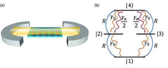
Figure 1: (a) Schematic of a laser composed of nanocrystal quantum dots coupled to an optical cavity. (b) Level diagram for a four-level model of a nanocrystal quantum dot.

Figure 1(a) illustrates the general model for a nanocrystal quantum dot laser. The laser is composed of an ensemble of quantum dots coupled to a single cavity mode. The level structure of the quantum dots, shown in Fig. 1(b), consists of four states: a ground state $|1\rangle$ which contains no carriers, the single exciton states $|2\rangle$ and $|3\rangle$ which contain a single electron-hole pair, and the biexciton state $|4\rangle$ which contains two electron-hole pairs. In the single exciton states, the quantum dot absorbs and emits a photon with nearly equal probability. Thus, only the biexciton state can provide optical gain  Klimov2003 . However, this state suffers from Auger recombination where an electron-hole pair recombines and transfers energy non-radiatively to a third carrier Klimov2000a . The strong carrier confinement in the quantum dots leads to fast Auger recombination, resulting in a low biexciton radiative efficiency.

Figure  1(b) also shows the relevant decay rates for our quantum dot model. The biexciton state decays to each exciton state with the rate $\gamma_{2}=\gamma_{0}+\gamma_{a}/2$, where $\gamma_{0}$ is the spontaneous emission rate and $\gamma_{a}$ is the total Auger recombination rate of the biexciton state. We assume the single exciton states decay predominantly by spontaneous emission. We also assume equal spontaneous emission rates for all four allowed transitions, and ignore long-lived trap states that are responsible for blinking behavior Nirmal1996 ; Jones2003 . These states can be incorporated as additional energy levels in the model. The quantum dot is incoherently pumped with an external source characterized by the excitation rate $R$.

In bare nanocrystal quantum dots Auger recombination is an order of magnitude faster than spontaneous emission Klimov2000a . It therefore dominates the decay of the biexciton state and quenches the optical gain. However, when the quantum dot spectrally couples to an optical cavity, its spontaneous emission rate increases by the factor  Gerard2003 .

$$F(\mathbf{r}_{0})=1+\frac{2g^{2}(\mathbf{r}_{0})}{\gamma_{0}K_{XX}}$$ (1)

where $g(\mathbf{r}_{0})$ is the cavity-quantum dot coupling strength given by

$$g(\mathbf{r}_{0})=\frac{\mathbf{\mu}\cdot\mathbf{\hat{e}}}{\hbar}\sqrt{\frac{\hbar\omega_{c}}{2\epsilon_{0}V_{m}}}\frac{|E(\mathbf{r}_{0})|}{|E(\mathbf{r})|_{max}}$$ (2)

Here, $E(\mathbf{r}_{0})$ is the electric field amplitude, $\mathbf{\hat{e}}$ is the polarization direction of the cavity mode at the quantum dot position $\mathbf{r}_{0}$, $\omega_{c}$ is the cavity mode resonant frequency, $V_{m}=\int d^{3}\mathbf{r}\epsilon(\mathbf{r})|E(\mathbf{r})|^{2}/[|E(\mathbf{r})|^{2}]_{max}$ is the cavity mode-volume  Zhang2011 , $\epsilon_{0}$ is the permittivity of free space, $\epsilon(\mathbf{r})$ is the relative dielectric permittivity and $\mathbf{\mu}$ is the quantum dot dipole moment. The rate $K_{XX}=(\gamma_{0}+2\gamma_{2}+\gamma_{d})/2$ represents the total linewidth of the biexciton state, which is dominated by the dephasing rate $\gamma_{d}$ at room-temperature  VanSark2001 ; Lounis2000 ; Klimov2000a . We note that Eq. (1) is different from the more common expression for $F$ that depends on the ratio of the cavity quality factor $Q$ and the cavity mode-volume $V_{m}$ Purcell1946 ; Gerard2003 . This difference occurs because at room temperature the dephasing rate of nanocrystal quantum dots is much larger than the cavity linewidth. The device therefore operates in the bad emitter regime, where $F$ becomes independent of the cavity $Q$. By engineering cavities with small mode-volumes, we can achieve large $F$ and enhance the spontaneous emission rate, thereby increasing the radiative efficiency of the quantum dot in the presence of Auger recombination.

To analyze the nanocrystal quantum dot laser in the presence of Auger recombination and spontaneous emission enhancement, we begin with the master equation

$$\frac{\partial\rho}{\partial t}=\frac{i}{\hbar}[\rho,\mathbf{H}]+\mathbf{L}\rho$$ (3)

where $\rho$ is the density matrix of the combined cavity-quantum dot system, $\mathbf{H}$ is the Hamiltonian, and $\mathbf{L}$ is the Liouvillian superoperator that accounts for incoherent damping and excitation processes. The Hamiltonian of the system is given by $\mathbf{H_{cavity}}+\mathbf{H_{NQD}}+\mathbf{H_{JC}}$, where

$$\mathbf{H_{cavity}} = \hbar\omega_{c}\mathbf{a}^{\dagger}\mathbf{a}$$ (4)

$$\mathbf{H_{NQD}} = \sum_{m=1}^{N}\hbar\omega^{X}_{m}(\sigma_{22,m}+\sigma_{33,m})+\hbar\omega^{XX}_{m}\sigma_{44,m}$$ (5)

$$\mathbf{H_{JC}} = \sum_{i=m}^{N}\hbar g^{X}_{m}(\mathbf{r}_{m})(\sigma_{21,m}\mathbf{a}+\sigma_{12,m}\mathbf{a}^{\dagger}+\sigma_{31,m}\mathbf{a}+\sigma_{13,m}\mathbf{a}^{\dagger})$$ (6)

$$+ \hbar g^{XX}_{m}(\mathbf{r}_{m})(\sigma_{42,m}\mathbf{a}+\sigma_{24,m}\mathbf{a}^{\dagger}+\sigma_{43,m}\mathbf{a}+\sigma_{34,m}\mathbf{a}^{\dagger})$$

In the above equations $\mathbf{a}$ and $\mathbf{a}^{\dagger}$ are the bosonic annihilation and creation operators of the cavity mode. The summation is carried out over all quantum dots in the cavity, where we denote the total number of quantum dots by $N$. For the $m^{th}$ quantum dot, $\sigma_{jk,m}=|j\rangle\langle k|$ represents the atomic dipole operator when $j\neq k$ and the atomic population operator when $j=k$, for the single exciton states ($j=2,3$) and the biexciton state ($j=4$). We set the energy of the quantum dot ground state to zero. We define $\omega^{X}_{m}$ and $\omega^{XX}_{m}$ as the resonant frequencies of the single-exciton and biexciton transitions, respectively. Similarly, the cavity-quantum dot coupling strengths for the exciton and biexciton transitions are $g^{X}_{m}(\mathbf{r}_{m})$ and $g^{XX}_{m}(\mathbf{r}_{m})$ for the $m^{th}$ quantum dot at position $\mathbf{r}_{m}$. At room temperature, the homogenous linewidth of these quantum dots is much larger than the biexcitonic shift Caruge2004 ; Empedocles1996 ; Empedocles1999 ; Norris1996 . We therefore assume all four transitions of each quantum dot are resonantly coupled to the cavity mode ($\omega_{c}=\omega^{X}_{m}=\omega^{XX}_{m}/2$). The Liouvillian superoperator $\mathbf{L}$ is fully defined in Appendix  A.

The master equation is difficult to solve both analytically and numerically when the number of quantum dots becomes large. However, we can simplify the calculations by applying the semi-classical approximation in which the coherence between the atoms and the field is neglected  WallsMilburn2007 ; Benson1999 and the density matrix can be factorized into a product of the state of the field and atoms (see Appendix  B). Under this approximation, the system is described by the average cavity photon number, $p$, and the quantum dot population density, $n_{j}(\mathbf{r})=\lim_{\Delta V\to 0}\sum_{m}\langle\sigma_{jj}^{m}\rangle/\Delta V$, where the sum is carried out over all quantum dots contained in a small volume $\Delta V$ at location $\mathbf{r}$. We note that $n_{j}(\mathbf{r})$ is a function of the position $\mathbf{r}$ inside the cavity because of the non-uniform cavity field distribution. We derive the equations of motion of $n_{j}(\mathbf{r})$ from the master equation (see Appendix  B) as

$${\partial n_{1}(\mathbf{r})\over\partial t} = \Gamma_{X}(\mathbf{r})[(p+1)(n_{2}(\mathbf{r})+n_{3}(\mathbf{r}))-2pn_{1}(\mathbf{r})]+\gamma_{0}[n_{2}(\mathbf{r})+n_{3}(\mathbf{r})]-2Rn_{1}(\mathbf{r})$$ (7)

$${\partial n_{2}(\mathbf{r})\over\partial t} = -\Gamma_{X}(\mathbf{r})[(p+1)n_{2}(\mathbf{r})-pn_{1}(\mathbf{r})]+\Gamma_{XX}(\mathbf{r})[(p+1)n_{4}(\mathbf{r})-pn_{2}(\mathbf{r})]$$ (8)

$$- \gamma_{0}n_{2}(\mathbf{r})+\gamma_{2}n_{4}(\mathbf{r})+R[n_{1}(\mathbf{r})-n_{2}(\mathbf{r})]$$

$${\partial n_{3}(\mathbf{r})\over\partial t} = -\Gamma_{X}(\mathbf{r})[(p+1)n_{3}(\mathbf{r})-pn_{1}(\mathbf{r})]+\Gamma_{XX}(\mathbf{r})[(p+1)n_{4}(\mathbf{r})-pn_{3}(\mathbf{r})]$$ (9)

$$- \gamma_{0}n_{3}(\mathbf{r})+\gamma_{2}n_{4}(\mathbf{r})+R[n_{1}(\mathbf{r})-n_{3}(\mathbf{r})]$$

$${\partial n_{4}(\mathbf{r})\over\partial t} = -\Gamma_{XX}(\mathbf{r})[2(p+1)n_{4}(\mathbf{r})-p(n_{2}(\mathbf{r})+n_{3}(\mathbf{r}))]-2\gamma_{2}n_{4}(\mathbf{r})$$ (10)

$$+ R[n_{2}(\mathbf{r})+n_{3}(\mathbf{r})]$$

In the above equations, $\Gamma_{X}(\mathbf{r})=2g^{2}(\mathbf{r})/K_{X}$ and $\Gamma_{XX}(\mathbf{r})=2g^{2}(\mathbf{r})/K_{XX}$ are the modified spontaneous emission rates of the single-exciton and biexciton transitions, where $K_{X}=(\gamma_{0}+\gamma_{d}+3R)/2$ and $K_{XX}=(\gamma_{0}+2\gamma_{2}+\gamma_{d}+R)/2$. Here, we assume equal coupling strength for the single-exciton and biexciton transitions. We also treat the quantum dots in a small volume $\Delta V$ of the cavity to be identical, and therefore drop the subscript $m$ from the coupling strength ($g(\mathbf{r})$ = $g^{X}_{m}(\mathbf{r}_{m})$ = $g^{XX}_{m}(\mathbf{r}_{m})$).

The average cavity photon number satisfies a rate equation given by (see Appendix  C for derivation)

$${\partial p\over\partial t}=-p\kappa+pG(p)+\alpha(p)$$ (11)

where $\kappa=\omega_{c}/Q$ is the cavity energy decay rate. The above equation is coupled to the quantum dot population density rate equations through the cavity gain coefficient

$$G(p)=\int d^{3}\mathbf{r}\left\{\Gamma_{X}(\mathbf{r})[n_{2}(\mathbf{r})+n_{3}(\mathbf{r})-2n_{1}(\mathbf{r})]+\Gamma_{XX}(\mathbf{r})[2n_{4}(\mathbf{r})-n_{2}(\mathbf{r})-n_{3}(\mathbf{r})]\right\}$$ (12)

and the spontaneous emission rate into the lasing mode

$$\alpha(p)=\int d^{3}\mathbf{r}\left\{\Gamma_{X}(\mathbf{r})[n_{2}(\mathbf{r})+n_{3}(\mathbf{r})]+2\Gamma_{XX}(\mathbf{r})n_{4}(\mathbf{r})\right\}$$ (13)

where the integral is over all space. We use the notation $G(p)$ and $\alpha(p)$ to highlight the fact that the above coefficients have a $p$ dependence because the atomic densities $n_{j}(\mathbf{r})$ depend on the cavity photon number. The absorbed pump power of the nanocrystal quantum dot laser is given by

$$P_{abs}=\hbar\omega_{p}R\int_{V_{p}}d^{3}\mathbf{r}[2n_{1}(\mathbf{r})+n_{2}(\mathbf{r})+n_{3}(\mathbf{r})]$$ (14)

where $\omega_{p}$ is the pump frequency and $V_{p}$ is the optically pumped volume. The output power of the laser is given by

$$P_{out}=\hbar\omega_{c}p\kappa$$ (15)

An important figure of merit for small mode-volume cavities is the spontaneous emission coupling efficiency, denoted by $\beta$. This parameter quantifies the fraction of photons spontaneously emitted to the cavity mode. A $\beta$ approaching unity achieves thresholdless lasing  Bjork1991 . In the quantum dot model, the single exciton and biexciton transitions have different coupling efficiencies given by

$$\beta_{X}(\mathbf{r}) = \frac{\Gamma_{X}(\mathbf{r})}{\Gamma_{X}(\mathbf{r})+\gamma_{0}}$$ (16)

$$\beta_{XX}(\mathbf{r}) = \frac{\Gamma_{XX}(\mathbf{r})}{\Gamma_{XX}(\mathbf{r})+\gamma_{2}}$$ (17)

The above coupling efficiencies depend on the position $\mathbf{r}$ due to the spatially varying cavity field intensity. The rate equations Eqs. (7)-(11) describe the dynamics of a general nanocrystal quantum dot laser. We will use these equations in the remaining sections.

III Lasing analysis under uniform-field approximation

The general cavity-quantum dot rate equation model, developed in the previous section, is still difficult to solve due to the spatial variation of the coupling strength $g(\mathbf{r})$. This spatial variation leads to a complex set of coupled differential equations for each position inside the cavity volume. We note that this complexity is not unique to the system we study. It occurs in virtually all laser systems and is responsible for effects such as spatial hole burning  MilonniEberlyBook . One way to simplify the problem is to make the uniform-field approximation, where we replace $\Gamma_{i}(\mathbf{r})$ (i = X, XX) in Eqs. (7)- (14) with its spatially averaged value

$$\bar{\Gamma}_{i}=\frac{1}{V_{m}}\int d^{3}\mathbf{r}\Gamma_{i}(\mathbf{r})=\frac{2g_{o}^{2}}{K_{i}}$$ (18)

where $g_{o}=\mathbf{\mu}\cdot\mathbf{\hat{e}}\sqrt{\omega_{c}/2\hbar\epsilon_{o}\epsilon_{eff}V_{m}}$ and

$$\epsilon_{eff}=\frac{\int d^{3}\mathbf{r}|E(\mathbf{r})|^{2}\epsilon(\mathbf{r})}{\int d^{3}\mathbf{r}|E(\mathbf{r})|^{2}}$$ (19)

Under the uniform field approximation the atomic population densities $n_{j}(\mathbf{r})$ are no longer spatially varying. We can therefore express the equations of motion in terms of the total number of quantum dots in state $j$ given by $N_{j}=V_{m}n_{j}$ where $V_{m}$ is the cavity mode volume. These quantum dot populations must satisfy the constraint that $\sum_{j}N_{j}=N$, where $N$ is the total number of quantum dots contained in the cavity. With these definitions, the equations of motion become the standard cavity-atom rate equations, given by

$${\partial{N}_{1}\over\partial t} = \bar{\Gamma}_{X}[(p+1)({N}_{2}+{N}_{3})-2p{N}_{1}]+\gamma_{0}({N}_{2}+{N}_{3})-2R{N}_{1}$$ (20)

$${\partial{N}_{2}\over\partial t} = -\bar{\Gamma}_{X}[(p+1){N}_{2}-p{N}_{1}]+\bar{\Gamma}_{XX}[(p+1){N}_{4}-p{N}_{2}]-\gamma_{0}{N}_{2}+\gamma_{2}{N}_{4}$$ (21)

$$+ R({N}_{1}-{N}_{2})$$

$${\partial{N}_{3}\over\partial t} = -\bar{\Gamma}_{X}[(p+1){N}_{3}-p{N}_{1}]+\bar{\Gamma}_{XX}[(p+1){N}_{4}-p{N}_{3}]-\gamma_{0}{N}_{3}+\gamma_{2}{N}_{4}$$ (22)

$$+ R({N}_{1}-{N}_{3})$$

$${\partial{N}_{4}\over\partial t} = -\bar{\Gamma}_{XX}[2(p+1){N}_{4}-p({N}_{2}+{N}_{3})]-2\gamma_{2}{N}_{4}+R({N}_{2}+{N}_{3})$$ (23)

$${\partial p\over\partial t} = -p\kappa+p\bar{G}(p)+\bar{\alpha}(p)$$ (24)

where

$$\bar{G}(p)=\bar{\Gamma}_{X}({N}_{2}+{N}_{3}-2{N}_{1})+\bar{\Gamma}_{XX}(2{N}_{4}-{N}_{2}-{N}_{3})$$ (25)

and

$$\bar{\alpha}(p)=\bar{\Gamma}_{X}({N}_{2}+{N}_{3})+2\bar{\Gamma}_{XX}{N}_{4}$$ (26)

are the gain coefficient and spontaneous emission rate into the lasing mode. The absorbed power is given by

$$\bar{P}_{abs}=\hbar\omega_{p}R(2{N}_{1}+{N}_{2}+{N}_{3})$$ (27)

The output power of the laser is still given by Eq. (15).

We first determine the minimum number of quantum dots required to achieve lasing. We define $N_{th}$ as the total number of quantum dots in the cavity required to achieve a small signal gain equal to the cavity loss ($\lim_{p\to 0}\bar{G}(p)=\kappa$), and calculate it by using the analytical steady-state solutions to Eqs. (20)- (23) along with the condition $\sum_{j}N_{j}=N$ (see Appendices  D, E). To perform calculations, we consider the specific example of colloidal CdSe/ZnS core-shell quantum dots that emit in a wavelength range of 500-700 nm. We perform simulations using a dephasing rate of $\gamma_{d}=$ 4.39$\times$10⁴ ns^-1 VanSark2001 , a spontaneous emission rate of $\gamma_{0}$ = $1/18$ ns^-1 Lounis2000 , and an Auger recombination rate of $\gamma_{a}$ = $1/300$ ps^-1 Klimov2000a ; Bruchez1998 . Nanocrystal quantum dots can be incorporated into photonic devices in a variety of ways such as spin-casting Min2006 ; Bose2007 ; Fushman2005 ; Rakher2011 ; Rakher2010 and immersion in liquid suspension  Wu2007 ; Snee2005 . In these cases, the quantum dots reside on the surfaces of the devices, so we set $\epsilon_{eff}=1$.

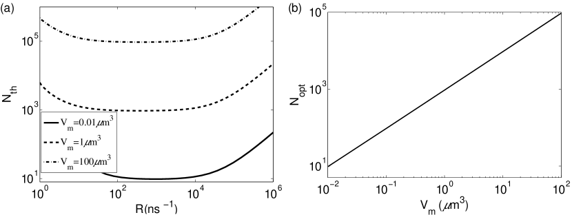
Figure 2: (a) $N_{th}$ as a function of pump rate for $V_{m}=0.01\mu m^{3}$, 1 $\mu m^{3}$ and 100$\mu m^{3}$, $\gamma_{a}$ = $1/300$ ps^-1. (b) $N_{opt}$ for different mode-volumes for $\gamma_{a}$ = $1/300$ ps^-1.

Figure 2(a) plots $N_{th}$ as a function of pump rate $R$ for $V_{m}=0.01\mu m^{3}$, 1$\mu m^{3}$ and 100$\mu m^{3}$ and $\gamma_{a}$ = $1/300$ ps^-1. Each mode-volume exhibits an optimum pump rate where the threshold quantum dot number is minimum. We denote this minimum threshold quantum dot number by $N_{opt}$. Figure 2(b) plots $N_{opt}$ as a function of $V_{m}$. The figure shows that $N_{opt}$ scales linearly with mode-volume.

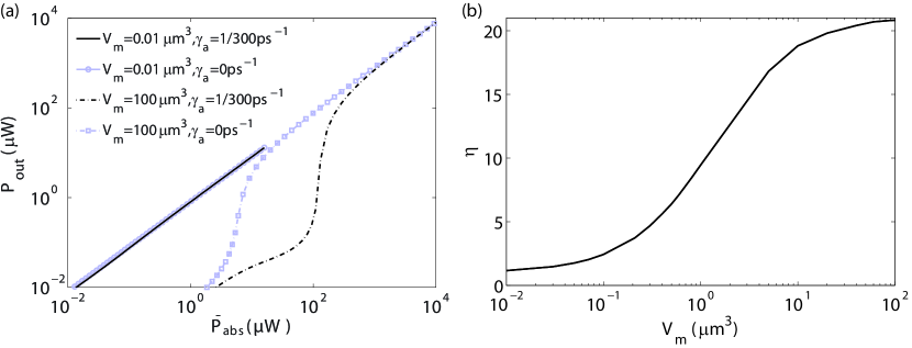
Figure 3: (a) Laser output power as a function of the absorbed pump power for $V_{m}=0.01\mu m^{3}$ and 100$\mu m^{3}$. (b)$\eta$ as a function of mode-volume.

Next, we investigate the laser input-output power characteristics. We calculate the laser output power (using Eq. (15)) and the absorbed pump power (using Eq. (27)) using the numerical steady-state solutions to Eqs. (20)-(24). Figure 3(a) plots $P_{out}$ as a function of $\bar{P}_{abs}$ (also known as the light-in light-out curve), under the uniform-field approximation, for two different mode-volumes of $V_{m}=$ 0.01 $\mu m^{3}$ and 100 $\mu m^{3}$, as well as two different Auger recombination rates of $\gamma_{a}$ = $1/300$ ps^-1 and $0$. We set $Q=$ 20000 and $N=2N_{opt}$ (Fig.  2(b)) for each respective mode-volume. We calculate the curves in Fig. 3(a) using the same range of $R$ values for both the mode-volumes. We note that the curves for the small mode volume cavity terminate earlier than those of the large mode volume cavity because the number of quantum dots contained inside the cavity mode-volume is much lower, which reduces the maximum output power.

The cavities with $V_{m}=$ 100$\mu$m³, indicated by the dashed curves in Fig. 3(a), exhibit a pronounced threshold. Near threshold, the light-in light-out curve takes on the well-known S-curve behavior as it transitions from the below-threshold to above-threshold regime. Auger recombination increases the threshold by quenching the gain, which causes the S-curve region to occur at higher absorbed powers. Similar to $N_{th}$, we define the threshold power as the absorbed power where the small signal gain equals the cavity loss. We calculate this value numerically using the steady state solutions to Eqs. (20)- (23), along with Eq. (27). The threshold power for $V_{m}=$ 100 $\mu m^{3}$ is 122.7 $\mu$W when $\gamma_{a}$ = $1/300$ ps^-1, and 5.9 $\mu$W when $\gamma_{a}$ = 0. Auger recombination therefore increases the lasing threshold by a factor of 21. When the mode volume is $V_{m}=$ 0.01 $\mu m^{3}$ the light-in light-out curve exhibits a thresholdless lasing behavior. The output power is nearly a linear function of the input power. Using the same definition of threshold, we determine the threshold powers with and without Auger recombination to be 97 nW and 84 nW respectively, corresponding to an increase of only 1.2. Thus, not only does the small mode volume cavity exhibit a much lower overall lasing threshold, but the lasing threshold is also largely unaffected by Auger recombination.

Figure 3(b) plots $\eta=P/P^{\prime}$ as a function of $V_{m}$, where $P$ is the absorbed pump power at threshold with $\gamma_{a}$ = $1/300$ ps^-1 and $P^{\prime}$ is the absorbed pump power at threshold with $\gamma_{a}$ = 0. We set the total quantum dot number in the cavities to $N=2N_{opt}$ for each value of $V_{m}$ (Fig.  2(b)). From this curve, we observe that below a mode-volume of 0.1 $\mu m^{3}$ the lasing threshold is largely unaffected by Auger recombination. Above this mode volume, $\eta$ rapidly increases and eventually reaches a saturated value. At large mode-volumes, $\eta$ becomes independent of the mode volume itself and achieves an asymptotic limit. From the upper and the lower limits of $\eta$ (21 and 1.2, respectively), we determine that spontaneous emission enhancement can reduce the lasing threshold up to a factor of 17.

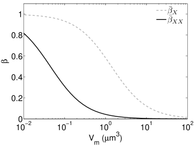
Figure 4: Spontaneous emission coupling efficiency for single-exciton transition $\bar{\beta}_{X}$ and biexciton transition $\bar{\beta}_{XX}$ as a function of $V_{m}$ for $\gamma_{a}$ = $1/300$ ps^-1

To verify that the improvement in lasing threshold is due to spontaneous emission enhancement, we calculate the spontaneous emission coupling efficiency for the exciton and biexciton transition as a function of $V_{m}$. Using the uniform field approximation, we replace $\Gamma_{i}(\mathbf{r})$ (i = X, XX) in Eqs. (16) - (17) with its spatially averaged value $\bar{\Gamma}_{i}$ which removes the spatial dependence and results in the simplified expressions for the coupling efficiencies given by

$$\bar{\beta}_{X} = \frac{\bar{\Gamma}_{X}}{\bar{\Gamma}_{X}+\gamma_{0}}$$ (28)

$$\bar{\beta}_{XX} = \frac{\bar{\Gamma}_{XX}}{\bar{\Gamma}_{XX}+\gamma_{2}}$$ (29)

Figure 4 plots spontaneous emission coupling efficiencies for the single-exciton transition $\bar{\beta}_{X}$ and the biexciton transition $\bar{\beta}_{XX}$ as a function of $V_{m}$ using $\gamma_{a}$ = $1/300$ ps^-1. At $V_{m}=$ 100 $\mu m^{3}$, $\bar{\beta}_{XX}$ is more than an order of magnitude smaller than $\bar{\beta}_{X}$. As the mode volume decreases the two efficiencies approach unity. The coupling efficiency of the biexciton transition begins to increase sharply and approach unity around the same mode-volume where $\eta$ (Fig. 3(b)) begins to saturate to unity. Thus, at small mode-volumes $\bar{\beta}_{XX}$ is insensitive to Auger recombination, and therefore the threshold pump power does not significantly change as indicated in Fig. 3(b).

IV Cavity device structure for low-threshold laser

The previous section established the advantage of using small mode-volume cavities to achieve low threshold lasing with nanocrystal quantum dots. A promising device structure for attaining this requirement is the nanobeam photonic crystal cavity. Nanobeam photonic crystal cavities have been previously studied in a variety of material systems, such as silicon Foresi1997 ; Deotare2009 ; Quan2011 , silicon nitride Eichenfield2009 ; Khan2011 , silicon dioxide Velha2007 ; Zain2008 ; Gong2010 , and gallium arsenide Rundquist2011 ; Rivoire2011 , and have been theoretically predicted to achieve mode-volumes approaching the diffraction limit  Deotare2009 ; Quan2011 ; Gong2010 ; Chan2009 .

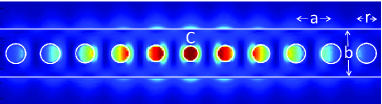
Figure 5: The electric field intensity ($|E|^{2}$) of the resonant cavity mode of a nanobeam photonic crystal cavity. The seven holes in the center form the cavity defect.

Figure  5 shows the nanobeam photonic crystal cavity design that we consider for low threshold lasing. Nanocrystal quantum dots are typically spin cast onto the device and therefore reside outside the dielectric. We therefore design the cavity mode to be localized in the air holes rather than the dielectric material. This design choice maximizes the field overlap with the quantum dots.

The structure is composed of a silicon nitride beam with a one-dimensional periodic array of air holes (radius $r=0.24a$, where $a$ is the lattice constant). The cavity is composed of a defect in the structure created by gradually reducing the radius of the three holes on either side of the hole labelled C to a minimum of $r_{0}$ = 0.2$a$. The adiabatic reduction of hole radius creates a smooth confinement for the photon and minimizes scattering due to edge states Quan2010 . The cavity is designed with beam thickness $d$ = 0.727$a$ and beam width $b$ = 1.163$a$. The index of refraction of silicon nitride is set to 2.01 Barth2007 . We calculate the mode of the cavity using three dimensional finite-difference time-domain simulation (Lumerical Solutions, Inc.). Figure 5 shows the calculated electric field intensity overlaid on the structure. The computed mode-volume is $V_{m}$ = 0.38$\lambda^{3}$ (= 0.11 $\mu m^{3}$) and the quality factor is $Q=64,000$.

Nanobeam photonic crystal cavities achieve mode-volumes that are on the order of a cubic wavelength. When the confinement volume of the cavity approaches the spatial variation of the field distribution, the uniform-field approximation can break down. We therefore analyze the nanobeam laser both with and without this approximation. We calculate $\epsilon_{eff}=1.9$ for the cavity by numerically integrating Eq. (19) using the computed electric field intensity profile of the simulated cavity structure (Fig. 5). Calculations under the uniform-field approximation follow the same approach as in the section III.

In order to investigate the input-output characteristics of the nanobeam laser without the uniform-field approximation, we first determine the total number of quantum dots required for achieving lasing threshold. We assume a uniform volume-density of quantum dots, denoted by $n=N/V_{p}$ where $V_{p}$ is the volume of the optically pumped region. We assume quantum dots reside only in the air holes and on the top of the nanobeam, which are optically pumped with an illumination spot with a diameter of 690 nm, covering the central three holes of the cavity (Fig. 5). We divide the illuminated volume into small volume elements (with volume $\Delta V$ at location $\mathbf{r}$) and numerically solve Eqs. (7)- (10) and Eq. (12) in steady state, along with the conditions $\sum_{j}n_{j}(\mathbf{r})=n$ for each volume element, and numerically determine the required $n$ to achieve $\lim_{p\to 0}G(p)=\kappa$. We assume that absorption loss due to quantum dots outside of the excitation volume are negligible compared to other loss mechanisms in the cavity.

Using the same simulation parameters as in the previous section, we numerically calculate the minimum number of quantum dots required to achieve threshold to be $N_{opt}=60$. This number is nearly identical to the value calculated using the uniform-field approximation which is 62. Next, we calculate the light-in light out curve using Eq. (14) and Eq. (15) without the uniform-field approximation. As in the previous section, we set the total number of quantum dots to be $N=2N_{opt}$.

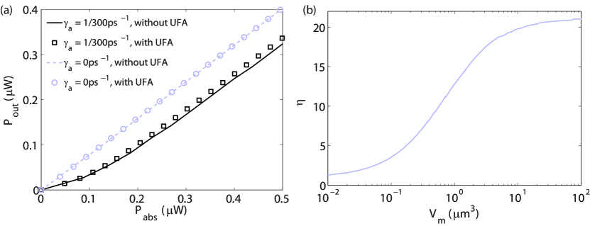
Figure 6: (a) Output power as a function of the absorbed pump power for nanocrystal quantum dot laser comprised of nanobeam photonic crystal cavity, using $\gamma_{a}=$ $1/300$ ps^-1 and 0, both with and without uniform-field approximation (abbreviated as UFA in the legend). (b) $\eta$ as a function of mode-volume under the uniform-field approximation for $\epsilon_{eff}=$ 1.9 and $Q=$ 64,000.

Figure 6(a) plots $P_{out}$ as a function of $P_{abs}$ for the nanobeam photonic crystal cavity with simulated $Q=64,000$ using $\gamma_{a}=$ $1/300$ ps^-1 and 0, both with and without the uniform-field approximation. The calculations show good agreement between the predicted input-output characteristics of the laser with and without the uniform-field approximation. Without the uniform-field approximation, the absorbed pump power at threshold for the nanobeam laser is 109.8 nW for $\gamma_{a}=$ $1/300$ ps^-1 and 29.9 nW for $\gamma_{a}=$ 0, resulting in $\eta$ = 3.7. With the uniform-field approximation, the absorbed pump power at threshold for the nanobeam laser is 112.6 nW for $\gamma_{a}=$ $1/300$ ps^-1 and 30 nW for $\gamma_{a}=$ 0, resulting in $\eta$ = 3.8.

The $\epsilon_{eff}$ for the nanobeam cavity, calculated from the cavity-field distribution, is 1.9. This calculated $\epsilon_{eff}$ is higher than the unity assumption in the previous section because in this realistic cavity design a fraction of the cavity field leaks into the dielectric medium (Fig. 5). Figure  6(b) plots $\eta$ as a function of $V_{m}$ under the uniform-field approximation for the same parameters used in Fig.  6(a). For a cavity with a mode volume of 100 $\mu m^{3}$, we determine that $\eta=$ 21.1. This value is 5.6 times larger than the value for the nanobeam cavity. Thus, the nanobeam cavity lasing threshold is much less sensitive to Auger recombination.

V Conclusion

In conclusion, we have theoretically shown that cavity-enhanced spontaneous emission of the biexciton reduces the effect of Auger recombination, leading to a lower lasing threshold. We developed a numerical model for a laser composed of an ensemble of nanocrystal quantum dots coupled to an optical cavity. The model can be expanded to incorporate more complex behavior of nanocrystal quantum dots, such as blinking, by introducing additional trap states into the quantum dot level structure  Zhao2010 ; Kuno2003 . This model can also be used to study lasing with other room-temperature emitters such as quantum rods  Kazes2002 ; HtoonPRL2003 , and other types of cavities such as plasmonic apertures  Choy2011 . Our results provide a direction for development of low-threshold and highly tunable nanolasers that use nanocrystal quantum dot as gain material at room temperature.

Appendices

Appendix A Liouvillian superoperator L

The Liouvillian superoperator $\mathbf{L}$ can be expressed as $\mathbf{L}=\mathbf{L_{NQD}}+\mathbf{L_{pump}}+\mathbf{L_{cavity}}$, where $\mathbf{L_{NQD}}$ accounts for the spontaneous relaxation of the quantum dot level structure, $\mathbf{L_{pump}}$ accounts for the incoherent pumping of the quantum dot population, and $\mathbf{L_{cavity}}$ accounts for the cavity decay. These operators are

$$\mathbf{L_{NQD}}\rho= \sum_{m=1}^{N} \frac{\gamma_{0,m}}{2}(2\sigma_{12,m}\rho\sigma_{21,m}-\sigma_{21,m}\sigma_{12,m}\rho-\rho\sigma_{21,m}\sigma_{12,m}$$ (30)

$$+ 2\sigma_{13,m}\rho\sigma_{31,m}-\sigma_{31,m}\sigma_{13,m}\rho-\rho\sigma_{31,m}\sigma_{13,m})$$

$$+ \frac{\gamma_{2,m}}{2}(2\sigma_{24,m}\rho\sigma_{42,m}-\sigma_{42,m}\sigma_{24,m}\rho-\rho\sigma_{42,m}\sigma_{24,m}$$

$$+ 2\sigma_{34,m}\rho\sigma_{43,m}-\sigma_{43,m}\sigma_{34,m}\rho-\rho\sigma_{43,m}\sigma_{34,m})$$

$$\mathbf{L_{pump}}\rho= \sum_{m=1}^{N} \frac{R}{2}(2\sigma_{21,m}\rho\sigma_{12,m}-\sigma_{12,m}\sigma_{21,m}\rho-\rho\sigma_{12,m}\sigma_{21,m}$$ (31)

$$+ 2\sigma_{31,m}\rho\sigma_{13,m}-\sigma_{13,m}\sigma_{31,m}\rho-\rho\sigma_{13,m}\sigma_{31,m}$$

$$+ 2\sigma_{42,m}\rho\sigma_{24,m}-\sigma_{24,m}\sigma_{42,m}\rho-\rho\sigma_{24,m}\sigma_{42,m}$$

$$+ 2\sigma_{43,m}\rho\sigma_{34,m}-\sigma_{34,m}\sigma_{43,m}\rho-\rho\sigma_{34,m}\sigma_{43,m})$$

$${\mathbf{L_{cavity}}\rho=\frac{\kappa}{2}(2\mathbf{a}\rho\mathbf{a}^{\dagger}-\mathbf{a}^{\dagger}\mathbf{a}\rho-\rho\mathbf{a}^{\dagger}\mathbf{a})}$$ (32)

The cavity energy decay rate is $\kappa=\omega_{c}/Q$.

Appendix B Equations of motion: projected on quantum dot levels

The equations of motion for the projections of $\rho$ on the levels (ij) of the $m^{th}$ quantum dot and photon states (pp’) $\rho_{ip,jp^{\prime}}^{m}=_{m}\langle i,p|\rho|j,p^{\prime}\rangle_{m}$ (i,j = 1 , 2, 3, 4) and ($p,p^{\prime}=0$ to $\infty$) are obtained using Eq. (3):

$$\frac{\partial\rho_{1p,1p}^{m}}{\partial t} = ig_{m}\sqrt{p}(\rho_{1p,2p-1}^{m}-\rho_{2p-1,1p}^{m}+\rho_{1p,3p-1}^{m}-\rho_{3p-1,1p}^{m})-2R\rho_{1p,1p}^{m}$$ (33)

$$+ \gamma_{0}(\rho_{2p,2p}^{m}+\rho_{3p,3p}^{m})+\kappa((p+1)\rho_{1p+1,1p+1}^{m}-p\rho_{1p,1p}^{m})$$

$$\frac{\partial\rho_{2p,2p}^{m}}{\partial t} = ig_{m}(\sqrt{p+1}(\rho_{2p,1p+1}^{m}-\rho_{1p+1,2p}^{m})+\sqrt{p}(\rho_{2p,4p-1}^{m}-\rho_{4p-1,2p}^{m}))$$ (34)

$$- (\gamma_{0}+R)\rho_{2p,2p}^{m}+R\rho_{1p,1p}^{m}+\gamma_{2}\rho_{4p,4p}^{m}+\kappa((p+1)\rho_{2p+1,2p+1}^{m}-p\rho_{2p,2p}^{m})$$

$$\frac{\partial\rho_{3p,3p}^{m}}{\partial t} = ig_{m}(\sqrt{p+1}(\rho_{3p,1p+1}^{m}-\rho_{1p+1,3p}^{m})+\sqrt{p}(\rho_{3p,4p-1}^{m}-\rho_{4p-1,3p}^{m}))$$ (35)

$$- (\gamma_{0}+R)\rho_{3p,3p}^{m}+R\rho_{1p,1p}^{m}+\gamma_{2}\rho_{4p,4p}^{m}+\kappa((p+1)\rho_{3p+1,3p+1}^{m}-p\rho_{3p,3p}^{m})$$

$$\frac{\partial\rho_{4p,4p}^{m}}{\partial t} = ig_{m}\sqrt{p+1}(\rho_{4p,2p+1}^{m}-\rho_{2p+1,4p}^{m}+\rho_{4p,3p+1}^{m}-\rho_{3p+1,4p}^{m})-2\gamma_{2}\rho_{3p,3p}^{m}$$ (36)

$$+ R(\rho_{2p,2p}^{m}+\rho_{3p,3p}^{m})+\kappa((p+1)\rho_{3p+1,3p+1}^{m}-p\rho_{3p,3p}^{m})$$

$$\frac{\partial\rho_{1p,2p-1}^{m}}{\partial t}=ig_{m}\sqrt{p}(\rho_{1p,1p}^{m}-\rho_{2p-1,2p-1}^{m})-K_{X}\rho_{1p,2p-1}^{m}$$ (37)

$$\frac{\partial\rho_{2p,4p-1}^{m}}{\partial t}=ig_{m}\sqrt{p}(\rho_{2p,2p}^{m}-\rho_{4p-1,4p-1}^{m})-K_{XX}\rho_{2p,4p-1}^{m}$$ (38)

$$\frac{\partial\rho_{1p,3p-1}^{m}}{\partial t}=ig_{m}\sqrt{p}(\rho_{1p,1p}^{m}-\rho_{3p-1,3p-1}^{m})-K_{X}\rho_{1p,3p-1}^{m}$$ (39)

$$\frac{\partial\rho_{3p,4p-1}^{m}}{\partial t}=ig_{m}\sqrt{p}(\rho_{3p,3p}^{m}-\rho_{4p-1,4p-1}^{m})-K_{XX}\rho_{3p,4p-1}^{m}$$ (40)

Here, $K_{X}\;=(\gamma_{0}+\gamma_{d}+3R)/2$ and $K_{XX}\;=(\gamma_{0}+2\gamma_{2}+\gamma_{d}+R)/2$ are the total relaxation rates of the diagonal terms, and $\gamma_{d}$ is the dephasing rate of the quantum dot (added phenomenologically). We set dephasing rate to be much greater than the cavity decay rate $\gamma_{d}\gg\kappa$, allowing us to drop the cavity decay contributions from the equations of motion of off-diagonal terms (Eqs. (37) - (40)). Large dephasing rate also allows us to adiabatically eliminate the expectation value $\langle\rho_{ip,jp^{\prime}}\rangle$ of the off-diagonal terms ($i\not=j$)from Eqs. (37) - (40), and reduces Eqs. (33) - (36) to

$$\frac{\partial\rho_{1p,1p}^{m}}{\partial t} = \frac{2g^{2}_{m}}{K_{X}}(\rho_{2p-1,2p-1}^{m}+\rho_{3p-1,3p-1}^{m}-2\rho_{1p,1p}^{m})p-2R\rho_{1p,1p}^{m}$$ (41)

$$+ \gamma_{0}(\rho_{2p,2p}^{m}+\rho_{3p,3p}^{m})+\kappa((p+1)\rho_{1p+1,1p+1}^{m}-p\rho_{1p,1p}^{m})$$

$$\frac{\partial\rho_{2p,2p}^{m}}{\partial t} = -\frac{2g^{2}_{m}}{K_{X}}(\rho_{2p,2p}^{m}-\rho_{1p+1,1p+1}^{m})(p+1)+\frac{2g^{2}_{m}}{K_{XX}}(\rho_{4p-1,4p-1}^{m}-\rho_{2p,2p}^{m})p$$ (42)

$$- (\gamma_{0}+R)\rho_{2p,2p}^{m}+\;R\rho_{1p,1p}^{m}+\gamma_{2}\rho_{4p,4p}^{m}+\kappa((p+1)\rho_{2p+1,2p+1}^{m}-p\rho_{2p,2p}^{m})$$

$$\frac{\partial\rho_{3p,3p}^{m}}{\partial t} = -\frac{2g^{2}_{m}}{K_{X}}(\rho_{3p,3p}^{m}-\rho_{1p+1,1p+1}^{m})(p+1)+\frac{2g^{2}_{m}}{K_{XX}}(\rho_{4p-1,4p-1}^{m}-\rho_{3p,3p}^{m})p$$ (43)

$$- (\gamma_{0}+R)\rho_{3p,3p}^{m}+\;R\rho_{1p,1p}^{m}+\gamma_{2}\rho_{4p,4p}^{m}+\kappa((p+1)\rho_{3p+1,3p+1}^{m}-p\rho_{3p,3p}^{m})$$

$$\frac{\partial\rho_{4p,4p}^{m}}{\partial t} = -\frac{2g^{2}_{m}}{K_{XX}}(2\rho_{4p,4p}^{m}-\rho_{2p+1,2p+1}^{m}-\rho_{3p+1,3p+1}^{m})(p+1)-2\gamma_{2}\rho_{4p,4p}^{m}$$ (44)

$$+ R(\rho_{2p,2p}^{m}+\rho_{3p,3p}^{m})+\kappa((p+1)\rho_{4p+1,4p+1}^{m}-p\rho_{4p,4p}^{m})$$

Now, tracing over all the photon states in Eq. (41) - (44), and applying semi-classical approximation to factorize full density matrix element into quantum dot and field parts such that $\rho_{ip,ip}=\rho_{ii}\rho_{pp}$, we get

$$\frac{\partial\rho_{11}^{m}}{\partial t}=\frac{2g^{2}_{m}}{K_{X}}(\rho_{22}^{m}+\rho_{33}^{m}-2\rho_{11}^{m})\langle p\rangle+\frac{2g^{2}}{K_{X}}(\rho_{22}^{m}+\rho_{33}^{m})-2R\rho_{11}^{m}+\gamma_{0}(\rho_{22}^{m}+\rho_{33}^{m})$$ (45)

$$\frac{\partial\rho_{22}^{m}}{\partial t} = -\frac{2g^{2}_{m}}{K_{X}}(\rho_{22}^{m}-\rho_{11}^{m})\langle p\rangle+\frac{2g^{2}_{m}}{K_{XX}}(\rho_{44}^{m}-\rho_{22}^{m})\langle p\rangle-\frac{2g^{2}_{m}}{K_{X}}\rho_{22}^{m}+\frac{2g^{2}_{m}}{K_{XX}}\rho_{44}^{m}$$ (46)

$$- (\gamma_{0}+R)\rho_{22}^{m}+R\rho_{11}^{m}+\gamma_{2}\rho_{44}^{m}$$

$$\frac{\partial\rho_{33}^{m}}{\partial t} = -\frac{2g^{2}_{m}}{K_{X}}(\rho_{33}^{m}-\rho_{11}^{m})\langle p\rangle+\frac{2g^{2}_{m}}{K_{XX}}(\rho_{44}^{m}-\rho_{33}^{m})\langle p\rangle-\frac{2g^{2}_{m}}{K_{X}}\rho_{33}^{m}+\frac{2g^{2}_{m}}{K_{XX}}\rho_{44}^{m}$$ (47)

$$- (\gamma_{0}+R)\rho_{33}^{m}+R\rho_{11}^{m}+\gamma_{2}\rho_{44}^{m}$$

$$\frac{\partial\rho_{44}^{m}}{\partial t} = -\frac{2g^{2}_{m}}{K_{XX}}(2\rho_{44}^{m}-\rho_{22}^{m}-\rho_{33}^{m})\langle p\rangle-\frac{4g^{2}_{m}}{K_{XX}}\rho_{44}^{m}-2\gamma_{2}\rho_{44}^{m}+R(\rho_{22}^{m}+\rho_{33}^{m})$$ (48)

where $\langle p\rangle=\sum_{p}p\rho_{pp}$ is the mean photon number. We define $n_{j}(\mathbf{r})=\lim_{\Delta V\to 0}\sum_{m}\langle\sigma_{jj}^{m}\rangle/\Delta V$ as the quantum dot population density of the j^th lasing level where the sum is carried out over all quantum dots contained in small volume $\Delta V$ at location $\mathbf{r}$ and get Eqs. (7) - (10).

Appendix C Rate equation for mean cavity photon number

The rate equation for the mean cavity photon number is given by

$${\langle\dot{p}\rangle}=\sum_{p}p{\dot{\rho}_{pp}}$$ (49)

Using Eqs. (41) - (44)

$${\langle\dot{p}\rangle}=\sum_{m}\sum_{p}p \{ \frac{2g^{2}_{m}}{K_{X}}(\rho_{2p-1,2p-1}^{m}-\rho_{1p,1p}^{m})p-\frac{2g^{2}_{m}}{K_{X}}(\rho_{2p,2p}^{m}-\rho_{1p+1,1p+1}^{m})(p+1)$$ (50)

$$+ \frac{2g^{2}_{m}}{K_{X}}(\rho_{3p-1,3p-1}^{m}-\rho_{1p,1p}^{m})p-\frac{2g^{2}_{m}}{K_{X}}(\rho_{3p,3p}^{m}-\rho_{1p+1,1p+1}^{m})(p+1)$$

$$+ \frac{2g^{2}_{m}}{K_{XX}}(\rho_{4p-1,4p-1}^{m}-\rho_{2p,2p}^{m})p-\frac{2g^{2}_{m}}{K_{XX}}(\rho_{4p,4p}^{m}-\rho_{2p+1,2p+1}^{m})(p+1)$$

$$+ \frac{2g^{2}_{m}}{K_{XX}}(\rho_{4p-1,4p-1}^{m}-\rho_{3p,3p}^{m})p-\frac{2g^{2}_{m}}{K_{XX}}(\rho_{4p,4p}^{m}-\rho_{3p+1,3p+1}^{m})(p+1)$$

$$- \kappa(p\rho_{pp}-(p+1)\rho_{p+1p+1})\}$$

Applying semi-classical approximation to factorize full density matrix element into quantum dot and field parts $\rho_{ip,ip}=\rho_{ii}\rho_{pp}$, and identifying $\sum_{p=0}^{\infty}p\rho_{p,p}=\langle p\rangle$ gives

$${\langle\dot{p}\rangle} = -\kappa\langle p\rangle+\sum_{m}\{\frac{2g^{2}_{m}}{K_{X}}(\rho_{22}^{m}+\rho_{33}^{m}-2\rho_{11}^{m})\langle p\rangle+\frac{2g^{2}_{m}}{K_{XX}}(2\rho_{44}^{m}-\rho_{22}^{m}-\rho_{33}^{m})\langle p\rangle$$ (51)

$$+ \frac{2g^{2}_{m}}{K_{X}}(\rho_{22}^{m}+\rho_{33}^{m})+\frac{4g^{2}_{m}}{K_{XX}}\rho_{44}^{m}\}$$

Eq. (51) leads us to Eq. (11).

Appendix D Expression for $N_{j}$ under the uniform-field approximation

Assuming total number of quantum dots in the cavity, $N$, such that $\sum_{i}N_{i}=N$, Eqs.  (20)-(23) can be solved in the steady-state as

$$N_{1} = \left(\frac{(p+1)\bar{\Gamma}_{X}+\gamma_{0}}{p\bar{\Gamma}_{X}+R}\right)\frac{N}{2\zeta}$$ (52)

$$N_{2} = N_{3}=\frac{N}{2\zeta}$$ (53)

$$N_{4} = \left(\frac{p\bar{\Gamma}_{XX}+R}{(p+1)\bar{\Gamma}_{XX}+\gamma_{2}}\right)\frac{N}{2\zeta}$$ (54)

$$\zeta = \frac{(p+1)\bar{\Gamma}_{X}+\gamma_{0}}{2(p\bar{\Gamma}_{X}+R)}+1+\frac{p\bar{\Gamma}_{XX}+R}{2((p+1)\bar{\Gamma}_{XX}+\gamma_{2})}$$ (55)

where $\zeta$ is the ratio of the total quantum dot population to the total single-exciton quantum dot population.

Appendix E Quantum dot number required for achieving lasing threshold

Under uniform-field approximation

$$N_{th}=\frac{\omega_{c}}{Q}\left(\frac{\frac{\bar{\Gamma}_{X}+\gamma_{0}}{2R}+1+\frac{R}{2\bar{\Gamma}_{XX}+2\gamma_{2}}}{\bar{\Gamma}_{X}(1-\frac{\bar{\Gamma}_{X}+\gamma_{0}}{R})+\bar{\Gamma}_{XX}(\frac{R}{\bar{\Gamma}_{XX}+\gamma_{2}}-1)}\right)$$ (56)

References

- (1) M. T. Hill, “Nanophotonics: lasers go beyond diffraction limit,” Nature nanotechnology 4, 706–7 (2009).
- (2) S. Kita, S. Hachuda, S. Otsuka, T. Endo, Y. Imai, Y. Nishijima, H. Misawa, and T. Baba, “Super-sensitivity in label-free protein sensing using a nanoslot nanolaser,” Optics express 19, 17683–90 (2011).
- (3) P. L. Gourley, J. K. Hendricks, A. E. McDonald, R. G. Copeland, K. E. Barrett, C. R. Gourley, and R. K. Naviaux, “Ultrafast nanolaser flow device for detecting cancer in single cells,” Biomedical microdevices 7, 331–9 (2005).
- (4) W. J. Parak, D. Gerion, T. Pellegrino, D. Zanchet, C. Micheel, S. C. Williams, R. Boudreau, M. A. Le Gros, C. A. Larabell, and A. P. Alivisatos, “Biological applications of colloidal nanocrystals,” Nanotechnology 14, R15–R27 (2003).
- (5) L. Qu and X. Peng, “Control of photoluminescence properties of CdSe nanocrystals in growth,” Journal of the American Chemical Society 124, 2049–55 (2002).
- (6) A. P. Alivisatos, “Semiconductor clusters, nanocrystals, and quantum dots,” Science 271, 933 (1996).
- (7) V. I. Klimov, Semiconductor and Metal Nanocrystals: Synthesis and Electronic and Optical Properties (Marcel Dekker, New York, 2003).
- (8) H.-J. Eisler, V. C. Sundar, M. G. Bawendi, M. Walsh, H. I. Smith, and V. Klimov, “Color-selective semiconductor nanocrystal laser,” Applied Physics Letters 80, 4614 (2002).
- (9) P. T. Snee, Y. Chan, D. G. Nocera, and M. G. Bawendi, “Whispering-Gallery-Mode Lasing from a Semiconductor Nanocrystal/Microsphere Resonator Composite,” Advanced Materials 17, 1131–1136 (2005).
- (10) B. Min, S. Kim, K. Okamoto, L. Yang, A. Scherer, H. Atwater, and K. Vahala, “Ultralow threshold on-chip microcavity nanocrystal quantum dot lasers,” Applied Physics Letters 89, 191124 (2006).
- (11) V. I. Klimov, A. A. Mikhailovsky, S. Xu, A. Malko, J. A. Hollingsworth, C. A. Leatherdale, H.-J. Eisler, and M. G. Bawendi, “Optical Gain and Stimulated Emission in Nanocrystal Quantum Dots,” Science 290, 314–317 (2000).
- (12) V. I. Klimov, A. A. Mikhailovsky, D. W. McBranch, C. A. Leatherdale, and M. G. Bawendi, “Quantization of Multiparticle Auger Rates in Semiconductor Quantum Dots,” Science 287, 1011–1013 (2000).
- (13) H. Htoon, J. Hollingsworth, R. Dickerson, and V. Klimov, “Effect of Zero- to One-Dimensional Transformation on Multiparticle Auger Recombination in Semiconductor Quantum Rods,” Physical Review Letters 91, 1–4 (2003).
- (14) H. Htoon, J. A. Hollingworth, A. V. Malko, R. Dickerson, and V. I. Klimov, “Light amplification in semiconductor nanocrystals: Quantum rods versus quantum dots,” Applied Physics Letters 82, 4776 (2003).
- (15) M. Kazes, D. Lewis, Y. Ebenstein, T. Mokari, and U. Banin, “Lasing from Semiconductor Quantum Rods in a Cylindrical Microcavity,” Advanced Materials 14, 317 (2002).
- (16) S. A. Ivanov, J. Nanda, A. Piryatinski, M. Achermann, L. P. Balet, I. V. Bezel, P. O. Anikeeva, S. Tretiak, and V. I. Klimov, “Light Amplification Using Inverted Core/Shell Nanocrystals: Towards Lasing in the Single-Exciton Regime,” The Journal of Physical Chemistry B 108, 10625–10630 (2004).
- (17) J. Nanda, S. A. Ivanov, H. Htoon, I. Bezel, A. Piryatinski, S. Tretiak, and V. I. Klimov, “Absorption cross sections and Auger recombination lifetimes in inverted core-shell nanocrystals: Implications for lasing performance,” Journal of Applied Physics 99, 034309 (2006).
- (18) E. M. Purcell, “Spontaneous emission probabilities at radio frequencies,” Physics Review 69, 681 (1946).
- (19) V. I. Klimov, “From fundamental photophysics to multicolor lasing,” Los Alamos Science 28, 214–220 (2003).
- (20) M. Nirmal, B. O. Dabbousi, M. G. Bawendi, J. J. Macklin, J. K. Trautman, T. D. Harris, and L. E. Brus “Fluorescence intermittency in single cadmium selenide nanocrystals,” Nature 383, 802–804 (1996).
- (21) M. Jones, J. Nedeljkovic, R. J. Ellingson, A. J. Nozik, and G. Rumbles, “Photoenhancement of Luminescence in Colloidal CdSe Quantum Dot Solutions,” The Journal of Physical Chemistry B 107, 11346–11352 (2003).
- (22) J. Gerard, “Solid-state cavity-quantum electrodynamics with self-assembled quantum dots,” Topics of Applied Physics 90, 283–327 (2003).
- (23) Y. Zhang, I. Bulu, W.-M. Tam, B. Levitt, J. Shah, T. Botto, and M. Loncar, “High-Q/V air-mode photonic crystal cavities at microwave frequencies,” Optics express 19, 9371–7 (2011).
- (24) W. G. J. H. M. van Sark, P. L. T. M. Frederix, D. J. Van den Heuvel, H. C. Gerritsen, A. A. Bol, J. N. J. van Lingen, C. de Mello Donegá, and A. Meijerink, “Photooxidation and Photobleaching of Single CdSe/ZnS Quantum Dots Probed by Room-Temperature Time-Resolved Spectroscopy,” The Journal of Physical Chemistry B 105, 8281–8284 (2001).
- (25) B. Lounis, H. A. Bechtel, D. Gerion, P. Alivisatos, and W. E. Moerner, “Photon antibunching in single CdSe/ZnS quantum dot fluorescence,” Chemical Physics Letters 329, 399–404 (2000).
- (26) J.-M. Caruge, Y. Chan, V. Sundar, H. Eisler, and M. Bawendi, “Transient photoluminescence and simultaneous amplified spontaneous emission from multiexciton states in CdSe quantum dots,” Physical Review B 70, 1–7 (2004).
- (27) S. Empedocles, D. Norris, and M. Bawendi, “Photoluminescence Spectroscopy of Single CdSe Nanocrystallite Quantum Dots,” Physical review letters 77, 3873–3876 (1996).
- (28) S. A. Empedocles and M. G. Bawendi, “Influence of Spectral Diffusion on the Line Shapes of Single CdSe Nanocrystallite Quantum Dots,” The Journal of Physical Chemistry B 103, 1826–1830 (1999).
- (29) D. Norris and M. Bawendi, “Measurement and assignment of the size-dependent optical spectrum in CdSe quantum dots,” Physical Review B, 53, 16338–16346 (1996).
- (30) D. F. Walls and G. J. Milburn, Quantum Optics (Springer, 2007).
- (31) O. Benson and Y. Yamamoto, “Master-equation model of a single-quantum-dot microsphere laser,” Physical Review A 59, 4756–4763 (1999).
- (32) G. Bjork and Y. Yamamoto, “Analysis of semiconductor microcavity lasers using rate equations,” IEEE Journal of Quantum Electronics 27, 2386–2396 (1991).
- (33) P. W. Milonni and J. H. Eberly, Laser Physics (Wiley, Hoboken, New Jersey, 2010).
- (34) M. Bruchez, M. Moronne, P. Gin, S. Weiss, and A. P. Alivisatos, “Semiconductor nanocrystals as fluorescent biological labels,” Science 281, 2013–2016 (1998).
- (35) R. Bose, X. Yang, R. Chatterjee, J. Gao, and C. W. Wong, “Weak coupling interactions of colloidal lead sulphide nanocrystals with silicon photonic crystal nanocavities near 1.55 m at room temperature,” Applied Physics Letters 90, 111117 (2007).
- (36) I. Fushman, D. Englund, and J. Vuckovic , “Coupling of PbS quantum dots to photonic crystal cavities at room temperature,” Applied Physics Letters 87, 241102 (2005).
- (37) M. T. Rakher, R. Bose, C. W. Wong, and K. Srinivasan,“Fiber-based cryogenic and time-resolved spectroscopy of PbS quantum dots,” Optics Express 19, 1786 (2011).
- (38) M. T. Rakher, R. Bose, C. W. Wong, and K. Srinivasan, “Spectroscopy of 1.55m PbS quantum dots on Si photonic crystal cavities with a fiber taper waveguide,” Applied Physics Letters 96, 161108 (2010).
- (39) Z. Wu, Z. Mi, P. Bhattacharya, T. Zhu, and J. Xu, “Enhanced spontaneous emission at 1.55 m from colloidal PbSe quantum dots in a Si photonic crystal microcavity,” Applied Physics Letters 90, 171105 (2007).
- (40) J. S. Foresi, P. R. Villeneuve, J. Ferrera, E. R. Thoen, G. Steinmeyer, S. Fan, J. D. Joannopoulos, L. C. Kimerling, Henry I. Smith, and E. P. Ippen, “Microcavities in optical waveguides,” Nature 390, 143–145 (1997).
- (41) P. B. Deotare, M. W. McCutcheon, I. W. Frank, M. Khan, and M. Lončar, “High quality factor photonic crystal nanobeam cavities,” Applied Physics Letters 94, 121106 (2009).
- (42) Q. Quan and M. Loncar, “Deterministic design of wavelength scale, ultra-high Q photonic crystal nanobeam cavities,” Optics Express 19, 18529–18542 (2011).
- (43) M. Eichenfield, R. Camacho, J. Chan, K. J. Vahala, and O. Painter, “A picogram- and nanometre-scale photonic-crystal optomechanical cavity,” Nature 459, 550–5 (2009).
- (44) M. Khan, T. Babinec, M. W. McCutcheon, P. Deotare, and M. Loncar, “Fabrication and characterization of high-quality-factor silicon nitride nanobeam cavities,” Optics letters 36, 421–3 (2011).
- (45) P. Velha, E. Picard, T. Charvolin, E. Hadji, J. C. Rodier, P. Lalanne, and D. Peyrade, “Ultra-High Q/V Fabry-Perot microcavity on SOI substrate,” Optics express 15, 16090–6 (2007).
- (46) A. R. Zain, N. P. Johnson, M. Sorel, and R. M. De La Rue, “Ultra high quality factor one dimensional photonic crystal/photonic wire micro-cavities in silicon-on-insulator (SOI),” Optics express 16, 12084–9 (2008).
- (47) Y. Gong and J. Vučković, “Photonic crystal cavities in silicon dioxide,” Applied Physics Letters 96, 031107 (2010).
- (48) A. Rundquist, A. Majumdar, and J. Vučković, “Off-resonant coupling between a single quantum dot and a nanobeam photonic crystal cavity,” Applied Physics Letters 99, 251907 (2011).
- (49) K. Rivoire, S. Buckley, and J. Vučković, “Multiply resonant high quality photonic crystal nanocavities,” Applied Physics Letters 99, 013114 (2011).
- (50) J. Chan, M. Eichenfield, R. Camacho, and O. Painter, “Optical and mechanical design of a “ zipper ” photonic crystal optomechanical cavity” 17, 555–560 (2009).
- (51) Q. Quan, P. B. Deotare, and M. Loncar, “Photonic crystal nanobeam cavity strongly coupled to the feeding waveguide,” Applied Physics Letters 96, 203102 (2010).
- (52) M. Barth, J. Kouba, J. Stingl, B. Löchel, and O. Benson, “Modification of visible spontaneous emission with silicon nitride photonic crystal nanocavities,” Optics express 15, 17231–40 (2007).
- (53) J. Zhao, G. Nair, B. R. Fisher, and M. G. Bawendi, “Challenge to the Charging Model of Semiconductor-Nanocrystal Fluorescence Intermittency from Off-State Quantum Yields and Multiexciton Blinking,” Physical Review Letters 104, 1–4 (2010).
- (54) M. Kuno, D. Fromm, S. Johnson, A. Gallagher, and D. Nesbitt, “Modeling distributed kinetics in isolated semiconductor quantum dots,” Physical Review B 67, 1–15 (2003).
- (55) J. T. Choy, B. J. M. Hausmann, T. M. Babinec, I. Bulu, M. Khan, P. Maletinsky, A. Yacoby, and M. Lončar, “Enhanced single-photon emission from a diamond–silver aperture,” Nature Photonics 5, 738–743 (2011).