Infinite Mixed Membership Matrix Factorization

Abstract

Rating and recommendation systems have become a popular application area for applying a suite of machine learning techniques. Current approaches rely primarily on probabilistic interpretations and extensions of matrix factorization, which factorizes a user-item ratings matrix into latent user and item vectors. Most of these methods fail to model significant variations in item ratings from otherwise similar users, a phenomenon known as the “Napoleon Dynamite” effect. Recent efforts have addressed this problem by adding a contextual bias term to the rating, which captures the mood under which a user rates an item or the context in which an item is rated by a user. In this work, we extend this model in a nonparametric sense by learning the optimal number of moods or contexts from the data, and derive Gibbs sampling inference procedures for our model. We evaluate our approach on the MovieLens 1M dataset, and show significant improvements over the optimal parametric baseline, more than twice the improvements previously encountered for this task. We also extract and evaluate a DBLP dataset, wherein we predict the number of papers co-authored by two authors, and present improvements over the parametric baseline on this alternative domain as well.

I Introduction

Generating recommendations for users based on their previously revealed preferences and the ratings of similar users has increased in popularity as a machine learning problem, primarily due to the activities of internet companies such as Amazon, or the coverage of competitions such as the Netflix prize. Most of these methods have at their core a matrix factorization-based approach. We can view the users and their ratings for items as a $U\times M$ matrix R (subsequently referred to as the ratings matrix or the user-item matrix), which contains the ratings for $U$ users over $M$ items, and where every item is rated by at least one user. The idea is to factorize R into its latent factors: ${\bf R\approx A^{T}B}$, where ${\bf A}\in\mathbb{R}^{D\times U}$ is the latent user matrix, and ${\bf B}\in\mathbb{R}^{D\times M}$ is the latent item matrix. These lower dimensional representations reflect the intuition that ratings are based on a small number of factors (with dimension $D$), and the idea is to complete the matrix using this low-dimensional formulation, by taking the inner product between user and item latent factors for items not rated by users during the prediction or “matrix completion” step.

This general approach is also known as collaborative filtering, since one not only utilizes the user’s previous preferences but also the preferences of similar users (hence the “collaborative” aspect). Probabilistic formulations of matrix factorization for recommendation systems generally improve upon the performance of their non-probabilistic counterparts, by treating the latent factors as random variables. However, such methods are unable to model context explicitly, since most probabilistic models of this form generate the ratings from a normal distribution with the mean set to the inner product between the user and item latent factors. As a result, phenomena like the Napoleon Dynamite effect, originally proposed in the context of the Netflix prize, wherein certain movies (or more generally, items) receive high variance ratings from users that otherwise rate other items similarly (the movie Napoleon Dynamite being a prime example), cannot be handled well in the traditional probabilistic matrix factorization framework.

The recently proposed mixed membership matrix factorization (M³F) model [1] aims to tackle this problem by explicitly modeling ratings not only with static latent factors, but with an additional bias term that takes into account the context of the rating. M³F represents this bias term by modeling it through a type of mixed membership stochastic blockmodel: each user and each item can be represented as a discrete distribution over user and item topics, representing contexts or moods under which users rate items. When a user $u$ rates an item $j$, the contextual bias of this rating is a function of the user’s bias for the item’s topic for that particular rating (intuitively, the context under which item $j$ is being rated). It is also a function of the item’s bias for the user’s topic for that rating (intuitively, the mood of the user $u$ at the time of rating). Thus, M³F models a user’s rating for an item as a function of both the static latent factors and the user-item group and user group-item based contextual biases.

The M³F model however, is limited in the sense that the number of user and item topics for the contextual bias term is set beforehand and not learned from the data. In our proposed extension to this model, which we refer to as the infinite mixed membership matrix factorization model (iM³F), we sample the user and item topic assignments from an infinite-dimensional prior, allowing us to learn the optimal number of user and item topics from the data. Ideally, we would like the user and item topics to be shared across all users and items, but that each user and item maintain their own topic proportions over these topics. Thus, we propose to use a hierarchical Dirichlet process prior on the number of item and user topics, and sample assignments through a Chinese restaurant franchise representation. A Gibbs sampling procedure is derived and implemented for this model, and we evaluate its performance on two datasets from different domains: a movie ratings dataset (MovieLens), and a publication co-authorship database that we extracted ourselves from the DBLP database. Compared to the baseline M³F model on the former dataset, we decrease root mean square error (RMSE) by 0.0065, which is two times higher than M³F’s improvement over its baseline. We also significantly outperform M³F on the DBLP dataset.

II Related Work

As a way to attack recommender system problems, matrix factorization has been one of the popular approaches along with content-based filtering [2], and in recent years has proven to be the superior alternative of the two [3]. Probabilistic matrix factorization (PMF) was first introduced by Salakhutdinov and Mnih [4], whereby ratings are generated from a Gaussian with a mean computed as the dot product of the user and item latent factors, with fixed variance. A fully Bayesian version of PMF (BPMF) was subsequently proposed by the same authors [5], where they assumed the latent factors were themselves generated by Gaussian distributions, with normal-Wishart priors on the hyperparameters.

Our work is primarily based on extending the M³F model [1] . In M³F, the user and item latent factors are modeled as in BPMF, but when generating a rating, in addition to using the dot product of the latent factors as the mean, we add a contextual bias term. More formally, we generate a rating by a user $u$ for an item $j$ as:

$$r_{uj}\sim\mathcal{N}(\chi_{0}+c_{u}^{k}+d_{j}^{i}+{\bf a}_{u}\cdot{\bf b}_{j},\sigma^{2})$$ (1)

where $c_{u}^{k}$ is the latent rating bias of user $u$ under item topic $k$, $d_{j}^{i}$ denotes the bias for item $j$ under user topic $i$, $\chi_{0}$ is a fixed global bias, and ${\bf a}_{u}$ and ${\bf b}_{j}$ are the latent user and item factors respectively. The M³F framework’s concept of modeling user and item biases through user-item topic and item-user topic interactions is derived from mixed membership stochastic blockmodels (MMSBs) [6], which itself is influenced by the original mixed membership topic modeling framework [7], and stochastic block models [8, 9].

Collaborative topic regression [10] also combines matrix factorization and mixed membership topic modeling, but their method solves a different problem, the cold start issue of out-of-matrix predictions, rather than contextual bias.

There has been a good amount of work on general non-parametric techniques in matrix factorization and in particular, applications in collaborative filtering. However, all of these approaches focus on the parameters corresponding to the number of latent factors, and aim to learn the optimal latent dimension from the data. [11] do not use a probabilistic approach and instead use SVD, whereas [12, 13] adopt an Indian Buffett Process to model the latent factor dimensionality, and implement variational inference-based solutions. We note that such non-parametric approaches are orthogonal to our method, since they target the latent dimensionality, and can thus be easily integrated and combined with our approach.

III Approach

Our proposed method, iM³F, is based on extending the M³F approach for probabilistic modeling of recommendation systems. In iM³F, we add an infinite-dimensional prior for user and item topics. This extension is realized in our model by using a nonparametric Bayesian prior for the topic distributions, providing the model the ability to have a potentially infinite number of user and item topics. We present the schematic and symbolic views of our model, and derive a Gibbs sampling inference scheme using the Chinese restaurant representation of the nonparametric prior.

III-A Chinese Restaurants

The nonparametric prior on the mixtures over topics for users and items is motivated by its ability to allow the data to dictate the optimal number of user and item groups, instead of parameterizing these values beforehand. Using such a prior makes it unnecessary to conduct extensive “tuning” experiments for the number of topics, and is arguably conceptually simpler and more elegant. We provide a brief background of the ideas, with an emphasis on the intuition. For a more rigorous introduction, we refer the reader to [14]. For the purposes of exposition, we discuss the case of users being defined as mixtures over user topics (i.e., a user is defined as a mixture of various “moods”), and note that the item case is completely symmetrical.

In the finite case, we can represent this mixture as a multinomial distribution over the various user topics. The conjugate prior for a multinomial distribution is the Dirichlet distribution, sometimes seen as a “distribution over distributions” or a distribution over finitely many points on the real line. If we take the number of mixture components to infinity, then the conjugate prior becomes a Dirichlet process (DP) [15], a distribution over an infinitely fine-grained real line.

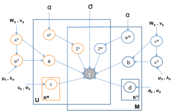
Figure 1: The original M³F model, as proposed in [1].

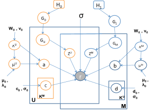
Figure 2: Our proposed iM³F model with an HDP prior on the user and item topics.

In practice, we do not have a density defined for the infinite-dimensional DP prior, so we define it indirectly via a sampling scheme that is used to generate samples from this prior [14]. If we are interested in both the weights and the partitions, then we use a stick-breaking construction to generate samples. Otherwise, if we are simply interested in partition or cluster assignments for the data, we can marginalize the mixture weights and sample the assignments directly, through a process known as a Chinese restaurant process (CRP) [16]. In our situation, for every rating $r_{uj}$, we can simply sample from the CRP prior to ascertain which item and user topics were used to generate the contextual bias for the rating.

A naive way to incorporate the CRP prior is to assume that each user and item maintain their own priors over item and user topics. Ideally though, we would like each user or item to maintain their own mixture weights over topics, but have a global set of topics that are shared across all users and items. This requirement necessitates a hierarchical Dirichlet process (HDP) prior [17] on the mixture components. In the Chinese restaurant metaphor, we now use a Chinese restaurant franchise (CRF) prior. Intuitively, this is a two-stage Dirichlet process, where we have one process for a global set of “dishes”, or topics that are shared by all users (or all items), and another user-specific process for the table assignments for individual customers (or ratings). The base distribution for each user-specific CRP is the process corresponding to the shared set of dishes, which forces each user (or item) to maintain a distribution over the shared set of topics.

III-B Generative Process

We present the generative process of the iM³F model, depicted in Figure 2. For the purposes of comparison, the schematic view of the finite, parametric case is presented in Figure 1, which corresponds to the original M³F model. First, the hyperparameters for the latent user and item factors are generated:

$$\Lambda^{U}\sim\textrm{Wishart}({\bf W}_{0},v_{0}),~{}\Lambda^{M}\sim\textrm{Wishart}({\bf W}_{0},v_{0})$$

$$\mu^{U}\sim\mathcal{N}(\mu_{0},(\lambda_{0}\Lambda^{U})^{-1}),~{}\mu^{M}\sim\mathcal{N}(\mu_{0},(\lambda_{0}\Lambda^{M})^{-1})$$

We also generate the global probability measures that are used to define a set of shared clusters for both the user and item topics:

$$G_{0}\sim\textrm{DP}(\beta,H_{0}),~{}G_{1}\sim\textrm{DP}(\beta,H_{1})$$

Note that we assume the DPs associated with the item and user global dishes have the same concentration parameter $\beta$, for the purposes of simplicity, and that the base measures are discrete and uniform. Now that we have the hyperparameters, we can sample the latent factor ${\bf a}_{u}$ for each user and the latent factor ${\bf b}_{j}$ for each item by sampling from a normal distribution. Furthermore, since we have the global base measures, we can sample the user- and item-specific mixture distributions from DPs with discrete base measures $G_{0}$ and $G_{1}$:

For each $$u\in\{1,\ldots,U\}:$$

$${\bf a}_{u}\sim\mathcal{N}(\mu^{U},(\Lambda^{U})^{-1})$$

$$G_{u}\sim\textrm{DP}(\gamma,G_{0})$$

For each $$j\in\{1,\ldots,M\}:$$

$${\bf b}_{j}\sim\mathcal{N}(\mu^{M},(\Lambda^{M})^{-1})$$

$$G_{j}\sim\textrm{DP}(\gamma,G_{1})$$

Once again, we assume the DPs associated with the item and user-specific mixtures have the same concentration parameter $\gamma$. With a slight abuse of notation, we can generate the user group and item group topic assignment indicator variables from CRPs with appropriate base distributions:

For each $$\textrm{rating }r_{uj}:$$

$$z_{uj}^{U}\sim\textrm{CRP}(\gamma,G_{u})$$

$$z_{uj}^{M}\sim\textrm{CRP}(\gamma,G_{j})$$

where $z_{uj}^{U}$ is the user cluster or topic that user $u$ belongs to when rating item $j$ (user $u$’s mood at the time of rating item $j$). Similarly, $z_{uj}^{M}$ is the item cluster or topic that item $j$, when rated by user $u$, belongs to. Note that in practice the topic assignments are sampled by marginalizing out the base distributions $G_{u}$ and $G_{j}$, and the only relevant parameter is $\gamma$, but for notational clarity we include the base measure. Letting $k=z_{uj}^{M}$ and $i=z_{uj}^{U}$, we can generate $c_{u}^{k}$, the bias of user $u$ for item topic $k$, and similarly generate $d_{j}^{i}$, the bias of a specific item $j$ for the user topic $i$ as follows:

$$d_{j}^{i}\sim\mathcal{N}(\mu_{i},\sigma_{0}^{2})$$

$$c_{u}^{k}\sim\mathcal{N}(\mu_{k},\sigma_{0}^{2})$$

Finally, we have all the pieces in place to generate the rating:

$$r_{uj}\sim\mathcal{N}(\beta_{uj}^{ik}+{\bf a}_{u}\cdot{\bf b}_{j},\sigma^{2})$$

where $\beta_{uj}^{ik}=\chi_{0}+c_{u}^{k}+d_{j}^{i}$.

III-C Inference via Gibbs Sampling

Our sampling procedure is similar to the M³F sampling scheme, except for the cluster assignment indicators $z^{U}$ and $z^{M}$, as they are generated from a CRF (in iM³F) instead of a multinomial with a Dirichlet prior.

We first sample the hyperparameters given the other variables in the model:

$$\Lambda^{U}|\textrm{rest}\backslash\{\mu^{U}\}\sim \textrm{Wishart}(({\bf W}_{0}^{-1}+\sum_{u=1}^{U}({\bf a}_{u}-\bar{\bf a})({\bf a}_{u}-\bar{\bf a})^{T})$$

$$+\frac{\lambda_{0}U}{\lambda_{0}+U}(\mu_{0}-\bar{\bf a})(\mu_{0}-\bar{\bf a})^{T})^{-1},\nu_{0}+U)$$ (2)

$$\Lambda^{M}|\textrm{rest}\backslash\{\mu^{M}\}\sim \textrm{Wishart}(({\bf W}_{0}^{-1}+\sum_{j=1}^{M}({\bf b}_{j}-\bar{\bf b})({\bf b}_{j}-\bar{\bf b})^{T})$$

$$+\frac{\lambda_{0}M}{\lambda_{0}+M}(\mu_{0}-\bar{\bf b})(\mu_{0}-\bar{\bf b})^{T})^{-1},\nu_{0}+M)$$ (3)

where in Equation 2, $\bar{\bf a}=\frac{1}{U}\sum_{u=1}^{U}{\bf a}_{u}$ and in Equation 3, $\bar{\bf b}=\frac{1}{U}\sum_{j=1}^{M}{\bf b}_{j}$. We then sample parameters $\mu^{U}$ and $\mu^{M}$:

$$\mu^{U}|\textrm{rest}\sim\mathcal{N}\left(\frac{\lambda_{0}\mu_{0}+\sum_{u=1}^{U}{\bf a}_{u}}{\lambda_{0}+U},(\Lambda^{U}(\lambda_{0}+U))^{-1}\right)$$

$$\mu^{M}|\textrm{rest}\sim\mathcal{N}\left(\frac{\lambda_{0}\mu_{0}+\sum_{j=1}^{M}{\bf b}_{j}}{\lambda_{0}+M},(\Lambda^{M}(\lambda_{0}+M))^{-1}\right)$$

Then, we sample the item bias for a given user $u$ and for $i\in\{1,\dots,K^{M}\}$:

$$c_{u}^{i}|\textrm{rest}\sim \mathcal{N}\left(\frac{\tfrac{c_{0}}{\sigma_{0}^{2}}+\sum_{j\in V_{u}}\sigma^{-2}z_{uji}^{M}\left(r_{uj}-\chi_{0}-d_{j}^{z_{uj}^{U}}-{\bf a}_{u}\cdot{\bf b}_{j}\right)}{\sigma_{0}^{-2}+\sum_{j\in V_{u}}\sigma^{-2}z_{uji}^{M}},\right.$$

$$\left.\frac{1}{\sigma_{0}^{-2}+\sum_{j\in V_{u}}\sigma^{-2}z_{uji}^{M}}\right)$$ (4)

where $V_{u}$ is the set of items rated by user $u$, and $z_{uji}^{M}$ is an selector variable which is 1 if the item topic assignment for user $u$ and item $j$ is $i$. Note that $K^{M}$ is conceptually infinite, but in practice we go through the item clusters that exist in the data thus far and generate $c^{i}_{u}$. Due to the symmetry of the user and item biases, the user bias for an item $j$, with $i\in\{1,\dots,K^{U}\}$ this time ($K^{U}$ is also conceptually infinite), is:

$$d_{j}^{i}|\textrm{rest}\sim \mathcal{N}\left(\frac{\tfrac{d_{0}}{\sigma_{0}^{2}}+\sum_{u:j\in V_{u}}\sigma^{-2}z_{uji}^{U}\left(r_{uj}-\chi_{0}-c_{u}^{z_{uj}^{M}}-{\bf a}_{u}\cdot{\bf b}_{j}\right)}{\sigma_{0}^{-2}+\sum_{u:j\in V_{u}}\sigma^{-2}z_{uji}^{U}},\right.$$

$$\left.\frac{1}{\sigma_{0}^{-2}+\sum_{u:j\in V_{u}}\sigma^{-2}z_{uji}^{U}}\right)$$ (5)

For notational convenience, let us define the empirical means and variances of the values sampled through Equations 4 and 5 as ($\mu_{c}$ , $\sigma_{c}$) and ($\mu_{d}$ , $\sigma_{d}$) respectively.

Using the conjugacy property of the Gaussian and Wishart distributions, we can sample the latent factors. We update ${\bf a}_{u}$ and ${\bf b}_{j}$ as follows:

For each $$u,$$

$${\bf a}_{u}|\textrm{rest}\sim \mathcal{N}\left((\Lambda_{u}^{U*})^{-1}\left(\Lambda^{U}\mu^{U}+\right.\right.$$

$$\left.\left.\sum_{j\in V_{u}}\sigma^{-2}{\bf b}_{j}\left(r_{uj}-\chi_{0}-c_{u}^{z_{uj}^{M}}-d_{j}^{z_{uj}^{U}}\right)\right),(\Lambda_{u}^{U*})^{-1}\right)$$ (6)

For each $$j,$$

$${\bf b}_{j}|\textrm{rest}\sim \mathcal{N}\left((\Lambda_{j}^{M*})^{-1}\left(\Lambda^{M}\mu^{M}+\right.\right.$$

$$\left.\left.\sum_{u:j\in V_{u}}\sigma^{-2}{\bf a}_{u}\left(r_{uj}-\chi_{0}-c_{u}^{z_{uj}^{M}}-d_{j}^{z_{uj}^{U}}\right)\right),(\Lambda_{u}^{U*})^{-1}\right)$$ (7)

where in Equation 6, $\Lambda_{u}^{U*}=\Lambda^{U}+\sum_{j\in V_{u}}\sigma^{-2}{\bf b}_{j}{\bf b}_{j}^{T}$, and in Equation 7, $\Lambda_{j}^{M*}=\Lambda^{M}+\sum_{u:j\in V_{u}}\sigma^{-2}{\bf a}_{u}{\bf a}_{u}^{T}$.

Finally, we draw the topic assignment indicators, which is where the HDP prior enters the picture. In the original M³F model, user and item topic assignment indicators $z_{uj}^{U}$ and $z_{uj}^{M}$ were sampled from a finite multinomial distribution, with the hyperparameters of this multinomial sampled from a Dirichlet prior multiplied by a likelihood term. In the CRF case, user topic and item topic assignment sampling is done via a two-stage process: sample the global dish assignments (per table) available to the franchise, and then sample the local table assignments (per customer) for a restaurant. Note that for the problem, it is not the entire rating that is modeled by the MMSB, but rather the rating residual, which is the rating minus the score predicted by the latent factors. Therefore, let the rating residual be defined as $x_{uj}=r_{uj}-\chi_{0}-{\bf a}_{u}\cdot{\bf b}_{j}$. Tying the restaurant analogy to our problem, customers are ratings (or rather, rating residuals, as only the $c$ and $d$ variables are affected by the topic assignments), tables are user-specific proportions over topics, and finally dishes are the topics themselves, in that they represent the parameters used to generate the data (residuals).

The corresponding Gibbs sampler thus has two sets of state variables: the first being the table assignment indicator $t$ of the observed residuals to tables, and the second is the dish assignment indicator $k$ associated with each table, which is just a group of residuals. We sample the table assignments as follows:

$$\mathbb{P}(t_{uj}=t) \propto N_{t}^{u,-j}\mathbb{P}(x_{uj}|\mu_{k_{t}}^{-uj})$$

$$\mathbb{P}(t=\bar{t}) \propto\gamma\left(\frac{\sum_{k=1}^{K}\mathbb{P}(x_{uj}|\mu_{k}^{-uj})M_{k}+\mathbb{P}(x_{uj}|c_{0})\beta}{\sum_{k=1}^{K}M_{k}+\beta}\right)$$

where $\bar{t}$ corresponds to sampling a new table, $\beta$ and $\gamma$ are the hyperparameters for the CRPs corresponding to the dish and table assignments respectively, $N_{t}^{u,-j}$ is the number of customers (rating residuals) associated with restaurant (user) $u$ sitting on existing table $t$ except the $j^{\textrm{th}}$ customer (i.e., except the rating residual of user $u$ for item $j$), and $M_{k}$ is the number of tables over all restaurants (users) on which the dish number $k$ is being served. In addition, $\mu_{k_{t}}^{-uj}$ is shorthand for the rating residual empirical mean, computed over all residuals across all users assigned to a table with dish $k$, except for the current residual that we are sampling for. $c_{0}$ is the prior for the bias or the residual term. When sampling a new table for a residual $x_{uj}$, if we happen to sample a previously nonexistent table, then we immediately sample a new dish for that table.

We sample dishes for each table as follows:

$$\mathbb{P}(k_{ut}=k)\propto M_{k}^{-ut}\prod_{t_{uj}=t}\mathbb{P}(x_{uj}|\mu_{k}^{-ut})$$ (8)

$$\mathbb{P}(k_{ut}=\bar{k})\propto\beta\prod_{t_{uj}=t}\mathbb{P}(x_{uj}|c_{0})$$ (9)

where $\bar{k}$ corresponds to sampling a new dish, $M_{k}^{-ut}$ represents the count of the tables assigned to dish $k$ except the current table that we are sampling a dish assignment for, and $\mu_{k}^{-ut}$ is shorthand for the rating residual empirical mean, computed over all residuals across all users assigned to a table with dish $k$ except all residuals on the current table we are sampling for. Note that when computing the likelihoods, we compute the joint likelihood over all the residuals associated with the current table, since in the dish assignment we assign a dish for a group of residuals.

When computing the probability of dish assignments as per Equations 8 and 9, we used the MAP estimate in the predictive likelihood term for our experiments (Section IV). To be completely Bayesian, the actual likelihood term is:

$$f({\bf x}_{t_{uj}=t}|\textrm{rest}) =\int\mathbb{P}(\mu_{k}^{-ut}|\{x_{u^{\prime}j^{\prime}}|k_{u^{\prime}j^{\prime}}=k,t_{u^{\prime}j^{\prime}}\neq t\})\cdot$$

$$\prod_{t_{uj}=t}\mathbb{P}(x_{uj}|\mu_{k}^{-ut})d\mu_{k}^{-ut}$$ (10)

$$=\int\mathbb{P}(\theta|\mathcal{X})\prod_{i=1}^{n}\mathbb{P}(x_{i}|\theta)d\theta$$ (11)

$$\propto\int\exp\left(\frac{-(\theta-\mu_{P})^{2}}{2\sigma_{P}^{2}}\right)\prod_{i=1}^{n}\exp\left(\frac{-(x_{i}-\theta)^{2}}{2\sigma^{2}}\right)d\theta$$ (12)

where in Equation 10, ${\bf x}_{t_{uj}=t}$ is the set of customers (residual ratings) sitting on table $t$ (the table we are sampling the dish for), and in Equation 11, $n$ is the number of customers (residuals) sitting on table $t$, $\mathcal{X}=\{x_{u^{\prime}j^{\prime}}|k_{u^{\prime}j^{\prime}}=k,t_{u^{\prime}j^{\prime}}\neq t\}$ is set of all other residuals across all users that are associated with dish or topic $k$ (index by $l$) except those sitting on our special table, and $\theta=\mu_{k}^{-ut}$. In Equation 12, we use the assumption that the data (residual) is generated from a Gaussian with a conjugate prior, and $\mu_{P}$ and $\sigma^{2}_{P}$ are defined as before. From Equation 12, we can say that the joint probability over $\mathbb{P}(\theta,{\bf x}_{t_{uj}=t})$ is a multivariate Gaussian, and marginalizing over $\theta$ yields a Gaussian as well. Using the laws of total expectation, variance, and covariance, one can show that:

$$\mathbb{E}[x_{i}|\mathcal{X}] = \mathbb{E}[\mathbb{E}[x_{i}|\theta,\mathcal{X}]|\mathcal{X}]=\mathbb{E}[\theta|\mathcal{X}]=\mu_{P}$$

$$\textrm{Var}[x_{i}|\mathcal{X}] = \textrm{Var}[\mathbb{E}[x_{i}|\theta,\mathcal{X}]|\mathcal{X}]+\mathbb{E}[\textrm{Var}[x_{i}|\theta,\mathcal{X}]|\mathcal{X}]$$

$$= \sigma^{2}+\sigma_{P}^{2}$$

$$\textrm{Cov}[x_{i},x_{j}|\mathcal{X}] = \mathbb{E}[\textrm{Cov}[x_{i},x_{j}|\theta,\mathcal{X}]|\mathcal{X}]+$$

$$\textrm{Cov}[\mathbb{E}[x_{i}|\theta,\mathcal{X}],\mathbb{E}[x_{j}|\theta,\mathcal{X}]|\mathcal{X}]$$

$$= 0+\textrm{Cov}[\theta,\theta]$$

$$= \textrm{Var}[\theta]=\sigma_{P}^{2}$$

Thus, we can write the predictive likelihood term as:

$$f({\bf x}_{t_{uj}=t}|\textrm{rest})\propto \frac{1}{|\sum|^{\frac{1}{2}}}\exp\left(-\frac{1}{2}({\bf x}_{t_{uj}=t}-\bm{\mu})^{T}\cdot\right.$$

$$\left.{\sum}^{-1}({\bf x}_{t_{uj}=t}-\bm{\mu})\right)$$ (13)

where $\bm{\mu}$ is an $n$-element vector with all entries equal to $\mu_{P}$ (the posterior mean), and $\sum$ is the covariance matrix for which all diagonal elements are equal to $\sigma^{2}+\sigma_{P}^{2}$ and all off diagonal elements are equal to $\sigma_{P}^{2}$.

We can also analytically obtain the determinant of the covariance matrix $\sum:\left|\sum\right|=\sigma^{2n}+n\sigma^{2(n-1)}\sigma_{P}^{2}$, where $n$ is the dimensionality of the matrix or the number of customers sitting at the table whose dish we are sampling for.

IV Experiments

The proposed iM³F model was evaluated on the MovieLens and DBLP datasets. On the MovieLens set, we broadly divided our results into internal comparisons, meaning hyperparameter variation experiments, and external comparisons, meaning the improvements vis-$\grave{\textrm{a}}$-vis M³F. For the DBLP dataset, we present final numbers in comparison to M³F. While previous work evaluated their approaches on the Netflix Prize dataset, we are unable to do so due to the unavailability of the data. All experiments were run on a quad-core 2.5 GHz Linux machine with 8GB RAM, and the implementation was done in MATLAB and C.

IV-A Datasets

The MovieLens dataset is a movie rating set, similar to those used in the Netflix prize. We used two versions of the datasets (ml100k and ml1m) that contain 100,000 and 1 million ratings respectively. Table I shows some summary statistics.

Name	Ratings	Users	Movies	Sparsity
ml100k	100,000	943	1682	6.3%
ml1m	1,000,000	6040	3952	4.2%

TABLE I: MovieLens Dataset Statistics. Sparsity refers to the percentage of non-zero elements in the matrix.

In both datasets, each user has rated at least 20 movies, with each rating being an integer from 1 to 5. When comparing the performance of different models, we measured the Root Mean Square Error (RMSE) on a held-out test set that is generated using a leave-one-out strategy: for each user, one random rating is chosen out of her movie ratings and put into the test set; the rest remain in the training set. We performed this random split twice, and all results for the MovieLens experiments are averaged over the two splits.

We have also extracted a publication dataset from the latest DBLP XML data as of January 6, 2013. The extracted co-authorship dataset can be made publicly available for comparison purposes. The dataset consists of around 4.5 million ratings; each rating is between two authors, and is simply a count of the number of papers that they have co-authored. For the purposes of our experiments, we selected the first 2 million ratings between 1 and 10, which consisted of 644,256 authors, and split the dataset into training and test components such that every author is represented at least once in the test set. In this dataset, the interpretation of the topics is akin to clusterings of researchers based on a specific sub-field, or geographical location.

IV-B Internal Comparisons

We use the ml100k dataset with 100 sampling iterations to look at how varying the hyperparameters $\beta$ and $\gamma$ affect the final number of topics estimated from the data. The larger ml1m dataset with 500 sampling iterations was used to evaluate RMSE for both the hyperparameter variation experiments and the final comparison with M³F. When comparing against M³F, we use the hyperparameter settings that yield the best performance as in the original paper [1]:

• Number of user topics $K^{U}$: 2

• Number of item topics $K^{M}$: 1

• Latent factor dimensionality $D$: 40

As we do not alter the latent factor terms, we maintain $D=40$ for the iM³F model.

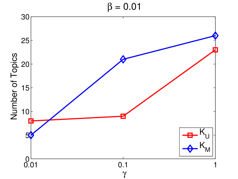
(a) Final topic number of CRF model, $\beta=0.01$

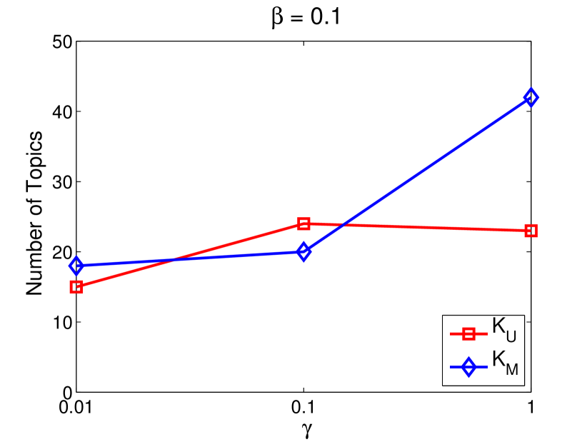
(b) Final topic number of CRF model, $\beta=0.1$

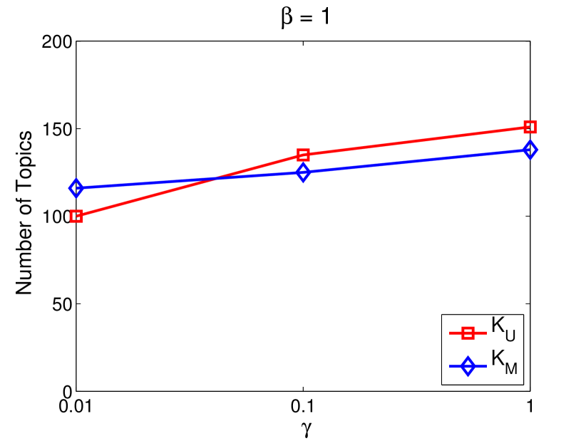
(c) Final topic number of CRF model, $\beta=1$

Figure 3: Impact of hyperparameters on CRF model

The impact of our CRF concentration parameters $\beta$ and $\gamma$, which correspond to the CRPs of the dish and table processes respectively, are presented in Figure 3. In Figures 3(a) to 3(c), we show the final topic numbers after running 100 iterations of the Gibbs sampler for the CRF model as we varied $\gamma$ and $\beta$. The overall trend is as expected, with higher $\beta$ and $\gamma$ values resulting in more topics.

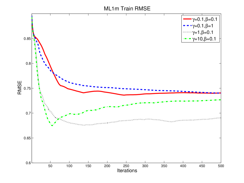
(a) ML1M, Train Set RMSE

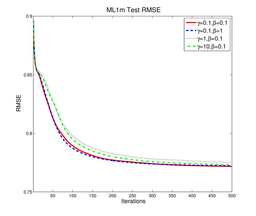
(b) ML1M, Test Set RMSE

Figure 4: RMSE comparison of various iM³F models.

Figure 4 presents the train and test set RMSE on ml1m for certain settings of the concentration parameters $\beta$ and $\gamma$. The lowest training RMSE was obtained when $\gamma=1,\beta=0.1$ (0.6904), with $K^{U}=94.5$ and $K^{M}=100$, which we refer to as ‘TrainBest’ in subsequent exposition. The lowest test RMSE was when $\gamma=0.1,\beta=0.1$ (0.7718), i.e., ’TestBest’, with $K^{U}=64$, and $K^{M}=77.5$.

IV-C iM³F and M³F

We then compared our CRF iM³F model with the M³F implementation of [1]. For the ml1m data, the M³F model also shows a better fit to the data, and achieves a much lower train RMSE of 0.60. However, in the test set comparison in Figure 5, both of our CRF models outperformed M³F after 500 rounds of Gibbs sampling. The final test RMSE for ‘TestBest’ (our best result) was 0.7718, while for the M³F model it was 0.7783, the difference being statistically significant according to the paired $t$-test. To put this improvement in context, the test set gain of 0.0065 is more than twice the improvement that M³F achieved over its baseline, BPMF, the difference between M³F and BPMF being the addition of the MMSB to model the contextual bias. ‘TrainBest’ achieved a test RMSE of 0.7750, also an improvement greater than the M³F-BPMF improvement.

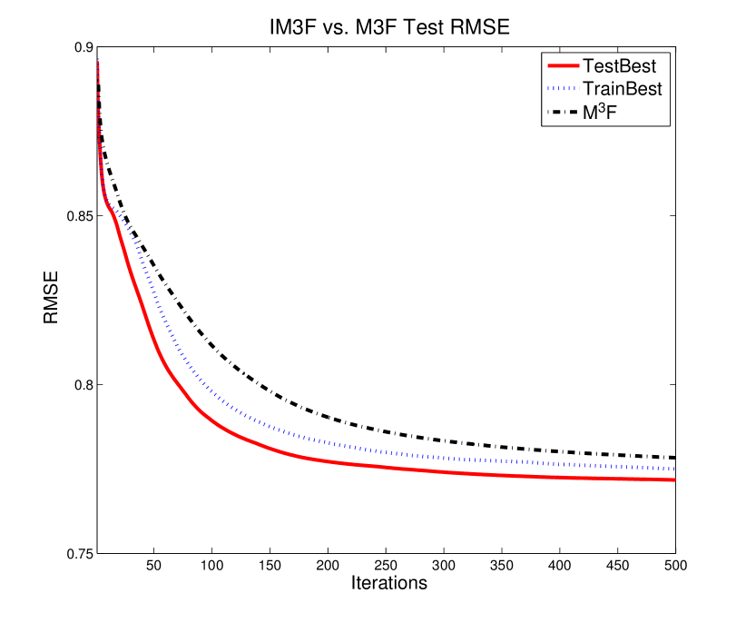
Figure 5: Test RMSE Comparison of iM3F and M3F model on the ml1m dataset.

Model	Train RMSE	Test RMSE	$K^{U}$	$K^{M}$
M3F	0.935	1.149	2	1
iM3F, $\gamma=0.1,\beta=0.1$	0.600	1.075	6	5
iM3F, $\gamma=0.1,\beta=1$	0.544	1.049	23	27

TABLE II: Final train and test set RMSE results on the DBLP dataset. Both iM³F models obtain better train and test set RMSE.

On the DBLP dataset, for M³F we carried out an extensive three-way grid search, varying the number of latent factors (with the values $\{5,10,15,20,25,30\}$), and user and item topics (with the values $\{1,2,4,8,16,32\}$), and found the best configuration to be $D=25,K^{U}=2,K^{M}=1$. The very fact that we had to implement an extensive grid search for these parameters already indicates the potential advantages of the nonparametric approach. For the iM³F model, guided by previous results we set $\gamma=0.1$ and tried $\beta=0.1$ and 1. The final results are presented in Table II, along with the final number of user and item topics. It is interesting to note that the number of user and item topics that achieved the best test RMSE in iM³F is quite a bit higher than the optimal parameters for M³F.

The performance gain achievable through iM³F comes at a cost, in that Gibbs sampling with nonparametric models is computationally more expensive than with parametric ones, as one always has to consider growing the number of clusters in light of more data. However, we note that recent efforts that develop exact, distributed MCMC procedures for Dirichlet process-based models [18] can easily be applied in our scenario to accelerate Gibbs sampling, which is a simple solution for today’s multicore computers. We emphasize however, that we have not added additional parameters to the model; rather, $K^{U}$ and $K^{M}$ have been replaced with a pair of hyperparameters, $\beta$ and $\gamma$, providing the model more flexibility to learn.

V Future Work & Conclusion

With the CRF prior, it is also possible to experiment with variants based on the nature of the data itself. For example, reciprocal datasets, wherein users rate other users ratings are based on mutual compatibility, are becoming increasingly more widespread, e.g., academic publication databases like our DBLP dataset or the Microsoft Academic Scholar database, or online dating websites like eHarmony or OkCupid. In the future, we would like to model the co-authorship dataset released (and other similar datasets) in more direct ‘relational’ manner. The bidirectional ratings need to be combined somehow to incorporate the principle of reciprocity in these ratings. Handling such modifications is straightforward in our work, e.g., Figure 6.

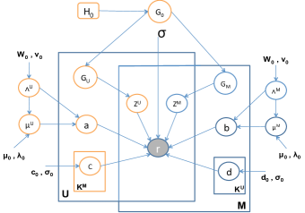
Figure 6: The iM³F model modified to handle reciprocity. We have a single user topic HDP prior shared on both sides of the rating.

In this paper, we designed and implemented an important addition to the general field of probabilistic matrix factorization. We proposed a nonparametric prior to the mixed membership matrix factorization model, and in the process derived a Gibbs sampler using a Chinese restaurant franchise representation. We then validated our model by decreasing RMSE on the MovieLens 1M dataset compared to M³F’s RMSE, a much more significant improvement than what had been done previously in the literature. We also extracted a co-authorship database from DBLP, and showed RMSE improvements over M³F there as well.

What the results suggest is that when utilizing and incorporating notions of mixed membership topic modeling into probabilistic matrix factorization, a nonparametric prior is a key assumption to make and model, let alone the convenience factor of not having to perform a grid search to find parameter values.

References

- [1] L. Mackey, D. Weiss, and M. I. Jordan, “Mixed membership matrix factorization,” in Proceedings of the 27th International Conference on Machine Learning, June 2010.
- [2] J. L. Herlocker, J. A. Konstan, L. G. Terveen, John, and T. Riedl, “Evaluating collaborative filtering recommender systems,” ACM Transactions on Information Systems, vol. 22, pp. 5–53, 2004.
- [3] Y. Koren, R. Bell, and C. Volinsky, “Matrix factorization techniques for recommender systems,” Computer, IEEE Computer Society, vol. 42, no. 8, pp. 30–37, Aug. 2009.
- [4] R. Salakhutdinov and A. Mnih, “Probabilistic matrix factorization,” in Advances in Neural Information Processing Systems, vol. 20, 2007.
- [5] ——, “Bayesian probabilistic matrix factorization using Markov chain Monte Carlo,” in Proceedings of the International Conference on Machine Learning, vol. 25, 2008.
- [6] E. M. Airoldi, D. M. Blei, S. E. Fienberg, and E. P. Xing, “Mixed membership stochastic blockmodels,” Journal of Machine Learning Research, vol. 9, pp. 1981–2014, Jun. 2008.
- [7] D. M. Blei, A. Y. Ng, and M. I. Jordan, “Latent Dirichlet Allocation,” Journal of Machine Learning Research, vol. 3, pp. 993–1022, Mar. 2003.
- [8] C. Kemp, J. B. Tenenbaum, T. Griffiths, T. Yamada, and N. Ueda, “Learning systems of concepts with an infinite relational model,” in Proceedings of the 21st National Conference on Artificial Intelligence, 2006.
- [9] K. Nowicki and T. A. B. Snijders, “Estimation and prediction for stochastic blockstructures,” Journal of the American Statistical Association, vol. 96, no. 455, pp. 1077–1087, 2001.
- [10] C. Wang and D. M. Blei, “Collaborative topic modeling for recommending scientific articles,” in Proceedings of the 17th ACM SIGKDD international conference on Knowledge discovery and data mining, ser. KDD ’11, 2011, pp. 448–456.
- [11] K. Yu, S. Zhu, J. Lafferty, and Y. Gong, “Fast nonparametric matrix factorization for large-scale collaborative filtering,” in Proceedings of the 32nd international ACM SIGIR conference on Research and development in information retrieval, ser. SIGIR ’09. New York, NY, USA: ACM, 2009, pp. 211–218.
- [12] N. Ding, Y. A. Qi, R. Xiang, I. Molloy, and N. Li, “Nonparametric bayesian matrix factorization by power-ep,” Journal of Machine Learning Research - Proceedings Track, vol. 9, pp. 169–176, 2010.
- [13] M. Xu, J. Zhu, and B. Zhang, “Nonparametric max-margin matrix factorization for collaborative prediction,” in NIPS, 2012, pp. 64–72.
- [14] H. Ishwaran and M. Zarepour, “Exact and approximate sum representations for the dirichlet process,” Canadian Journal of Statistics, vol. 30, no. 2, pp. 269–283, 2002.
- [15] T. S. Ferguson, “A Bayesian Analysis of Some Nonparametric Problems,” The Annals of Statistics, vol. 1, no. 2, pp. 209–230, 1973.
- [16] D. Blackwell and J. B. Macqueen, “Ferguson distributions via Pólya urn schemes,” The Annals of Statistics, vol. 1, pp. 353–355, 1973.
- [17] Y. W. Teh, M. I. Jordan, M. J. Beal, and D. M. Blei, “Hierarchical dirichlet processes,” Journal of the American Statistical Association, vol. 101, no. 476, pp. 1566–1581, 2006.
- [18] S. A. Williamson, A. Dubey, and E. P. Xing, “Exact and Efficient Parallel Inference for Nonparametric Mixture Models,” ICML 2013, 2013.