Numerical study of viscous starting flow past a flat plate

Abstract

Viscous flow past a finite flat plate which is impulsively started in direction normal to itself is studied numerically using a high order mixed finite difference and semi-Lagrangian scheme. The goal is to resolve details of the vorticity generation at early times, and to determine the effect of viscosity on flow quantities such as the core trajectory and vorticity, and the shed circulation. Vorticity contours, streaklines and streamlines are presented for a range of Reynolds numbers $Re\in[250,2000]$ and a range of times $t\in[0.0002,5]$. At early times, most of the vorticity is attached to the plate. The paper proposes a definition for the shed circulation at early as well as late times, and shows that it indeed represents vorticity that separates from the plate without reattaching. The contribution of viscous diffusion to the circulation shedding rate is found to be significant, but, interestingly, to depend only slightly on the value of the Reynolds number. The shed circulation and the vortex core trajectories follow scaling laws for inviscid self-similar flow over several decades in time. Scaling laws describing the core vorticity, core dissipation, boundary layer thickness, drag and lift forces in time and Reynolds number are also presented. The simulations provide benchmark results to evaluate, for example, simpler separation models such as point vortex and vortex sheet models.

1 Introduction

Vorticity separation in flow past sharp edges is a fundamental process of intrinsic interest in fluid dynamics. The boundary layer vorticity is convected around the edge, where it concentrates and forms a vortex. The vortex grows in strength and size, eventually causing the boundary layers to separate as a shear layer that rolls up in a spiral shape around the vortex core. The starting vortex flow has been the focus of many experimental, analytical and numerical studies, beginning with the work of Prandtl (see Lugt 1995). This paper concerns flow past a finite flat plate of zero thickness which is impulsively started in direction normal to itself. Closely related laboratory experiments include the works of [Pierce (1961)], [Taneda and Honji (1971)], [Pullin and Perry (1980)], [Lian and Huang (1989)], and [Lepage et al (2005)]. They visualize the rolled-up layer and yield data on the vortex size, core trajectory, core vorticity distribution, and the onset of an instability along the outer spiral turns. Related numerical results include the simulations of [Wang (2000)] and [Eldredge (2007)] for viscous flow past thin rounded plates, and those of [Hudson and Dennis (1985)] and [Dennis et al (1993)], followed by [Koumoutsakos and Shiels (1996)], and [Luchini and Tognaccini (2002)], for flow past plates of zero thickness. The first three of these consider finite plates, while [Luchini and Tognaccini (2002)] compute flow past a semi-infinite plate. These works report vortex fields, vortex core trajectories and induced forces at intermediate to relatively large times.

The main goal of this paper is to complement these earlier works with numerical results that yield new information about the flow, in particular on quantities that may be more difficult to measure experimentally. Our focus is to resolve the flow over several decades in time for a range of Reynolds numbers, show details of the vorticity generation and study the effect of viscosity on various flow quantities. Specific quantities of interest include the vortex trajectory, the forces induced by the wall vorticity, and the shed circulation. Computing shed circulation requires defining the region of entrainment of the starting vortex, which is not clearly apparent in the early formation stages. Once this region is determined, we investigate convective and diffusive contributions to the circulation shedding rate, and thereby obtain detailed insight into how viscosity affects circulation shedding. The computations also yield several scaling laws that show the dependence on time and Reynolds number for the corresponding quantities. While the results pertain to an idealized flow past a plate of zero thickness, they can be used as a basis of comparison to evaluate widely used low order models for separated flows, such as point vortex models (eg., Cortelezzi and Leonard 1993, Michelin and Llewellyn Smith 2009, Eldredge and Wang 2010, Ysasi et al 2011), or vortex sheet models (eg., Krasny 1991, Nitsche & Krasny 1994, Jones 2003, Jones and Shelley 2005, Alben and Shelley 2008, Shukla and Eldredge 2007), which are all based on simple approximations for the circulation shedding rate. The results also provide a basis of comparison to determine, for example, the effect of finite plate thickness, the shape of the plate tip (Schneider et al 2014), or the wedge angle in flow past wedges (Pullin & Perry 1980).

Impulsively started flow past a plate of zero thickness is difficult to compute for several reasons. The fluid velocity and shed vorticity are initially unbounded, requiring a fine mesh and small timesteps. Velocity and vorticity gradients near the wall are large, causing numerical instabilities. Here, we use a split method in time in which advection is treated using a semi-Lagrangian scheme, diffusion is treated with a 3-level Crank-Nicholson method, and all finite difference and interpolation approximations are of 4th order. The method uses ideas from several previous works, including [E and Liu (1996)], [Luchini and Tognaccini (2002)], [Staniforth and Cote (1991)], [Seaid (2002)], [Johnston (1999)], [Nitsche et al (2003)]. The method is of 2nd order for the present highly singular flow.

The simulations yield well resolved vorticity evolution profiles over a large range of times. Results are first presented for fixed Reynolds number $Re=500$, including details of the vorticity near the boundary. Following results using $Re\in[250,2000]$ show the dependence on $Re$. Based on the computed profiles, we define the separated vorticity at early times, when it is not clearly differentiated from boundary vorticity, and use this definition to compute shed circulation, as well as convective and diffusive components of the vorticity flux into the starting vortex. The results show that the chosen vortex boundary indeed bounds separated vorticity from vorticity that remains attached. They also show that viscous diffusion contributes significantly to the circulation shedding rate, but its contribution depends surprisingly little on the value of the Reynolds number. The shed circulation and the vortex core trajectory are found to follow inviscid scaling laws (Kaden 1931, Pullin 1978) over several decades in time. The computed trajectory is also in good agreement with experimental results of [Pullin and Perry (1980)]. The core vorticity and dissipation, and the induced drag and lift forces, are found to follow scaling laws that define their dependence on time and on $Re$.

The paper is organized as follows. Section 2 describes the problem of interest and the governing equations. Section 3 presents the numerical method, its accuracy, and the resolution obtained. Section 4 presents the numerical results, including the evolution in time for fixed $Re$, the dependence at a fixed time on $Re$, the core trajectory and vorticity, the circulation and circulation shedding rates, and the induced drag and lift forces, in that order. The results are summarized in section 5.

2 Problem Formulation

Figure 1: Sample solution at a relatively large time. (a) Streamlines. (b) Vorticity field. Positive vorticity contours are shown in black, negative ones in a lighter shade of grey.

2.1 Problem description

A finite plate of length $L$ and zero thickness is immersed in viscous fluid and impulsively started to move from zero velocity to a constant velocity $U>0$ in direction normal to itself. The flow is nondimensionalized using the plate length $L$ as the characteristic length scale, and $U$ as the characteristic velocity. An alternative nondimensionalization, appropriate in the absence of a length scale, or at very early times, is given by using $\nu/U$ instead of $L$ as the characteristic length scale, where $\nu$ is the kinematic fluid viscosity. This alternative is discussed in the Appendix.

The flow is assumed to be two dimensional. It is described in nondimensional Cartesian coordinates $\boldsymbol{x}=(x,y)$, and time $t$, with fluid velocity $\boldsymbol{u}(\boldsymbol{x},t)=\big{\langle}u(x,y,t),v(x,y,t)\big{\rangle}$. We choose a reference frame moving with the plate, in which the plate is positioned horizontally on the x-axis, centered at the origin, at

$$S=\Big{\{}(x,y):x\in\big{[}-\frac{1}{2},\frac{1}{2}\,\big{]}~{},~{}y=0~{}\Big{\}}~{},$$ (1)

the plate velocity is zero, and the far field velocity points upwards,

$$\boldsymbol{u}_{\infty}(t)=\big{\langle}0,1\big{\rangle}~{}.$$ (2)

To illustrate, figure 1 plots the streamlines and vorticity field at some relatively large time past the start of the motion. Here and throughout the paper, positive vorticity contours are shown in black, negative contours are shown in a lighter grey scale. The flow is assumed to remain symmetric about $x=0$, since at the times considered here symmetry breaking instabilities are not expected to significantly affect the flow. Hereafter, results are only shown for the right half plane, $x\geq 0$.

The flow is driven by the potential flow past the plate induced by the far field velocity. The corresponding stream function, $\psi_{\infty}(x,y)$, is given by the complex potential

$$W_{\infty}(x,y)=\sqrt{{1\over 4}-(x+iy)^{2}}=\phi_{\infty}+i\psi_{\infty}~{}.$$ (3)

This flow is induced by a vortex sheet in place of the plate whose strength is such that no flow passes through the plate. For higher generality, instead of using equation (3), we approximate $\psi_{\infty}$ using a sufficiently fine discretization of the vortex sheet, following the approach taken in Nitsche & Krasny (1994), which can be applied to other geometries as well, even if the analytic expression for the potential is not known.

2.2 Governing equations

The fluid flow is modeled by the incompressible Navier Stokes equations with constant density. The governing equations, given in terms of the fluid vorticity $\omega(\boldsymbol{x},t)=v_{x}-u_{y}$ and stream function $\psi(\boldsymbol{x},t)$, are

(a) $$\quad\frac{\partial\omega}{\partial t}+(\boldsymbol{u}\cdot\nabla)\omega=\frac{1}{Re}\nabla^{2}\omega,$$ (4a)

(b) $$\quad\nabla^{2}\psi=-\omega,~{}~{}\text{with}~{}~{}\psi=0~{}\text{on}~{}S~{}\text{and}~{}\psi\to\psi_{\infty}~{}\text{as}~{}\mathbf{x}\to\infty,$$ (4b)

(c) $$\quad\boldsymbol{u}=\nabla^{\perp}\psi,~{}~{}\text{with}~{}~{}\boldsymbol{u}=0~{}\text{on}~{}S~{},$$ (4c)

where $\nabla^{\perp}\psi=\big{\langle}\frac{\partial\psi}{\partial y},-\frac{\partial\psi}{\partial x}\big{\rangle}$, $Re=LU/\nu~{},$ and $\nu$ is the kinematic fluid viscosity.

3 Numerical Approach

3.1 Numerical Method

The numerical method is based on fourth order finite difference approximations of the governing equations on a regular grid. The computational domain is the rectangular region

$$D=[0,x_{\text{max}}]\times[y_{\text{min}},y_{\text{max}}]~{},$$ (5)

with symmetry imposed across $x=0$. The interior of the domain is given by the interior of $D\backslash S$, where $S$ is the plate position given in (1). The computational boundary consists of $\partial D\cup S$. Here $x_{\text{max}}>1/2$, $y_{\text{min}}<0$, $y_{\text{max}}>0$ are chosen sufficiently large so that the vorticity $\omega$ effectively vanishes on $\partial D$ for all the times computed. The domain is discretized by $(N_{x}+1)\times(N_{y}+1)$ equally spaced gridpoints $(x_{i},y_{j})$, where

$$x_{i} =ih~{},\hskip 22.76228pt\qquad i =0,\dots,N_{x}~{},\quad h=x_{\text{max}}/N_{x}~{},$$ (6a)

$$y_{j} =y_{\text{min}}+jk~{},\quad j =0,\dots,N_{y}~{},\quad k=(y_{\text{max}}-y_{\text{min}})/N_{y}~{},$$ (6b)

and $$N_{x},N_{y} h=k$$ are chosen so that . Similarly, time is discretized as

$$t_{n} =n\Delta t~{},\hskip 34.14322ptn =0,\dots,N~{},\quad\Delta t=T_{fin}/N~{},\hskip 48.36958pt$$ (6c)

where $T_{fin}=t_{N}$ is the final time. Streamfunction, velocity and vorticity are carried on the gridpoints, with $\psi_{i,j}^{n}$, $\langle u,v\rangle_{i,j}^{n}$, $\omega_{i,j}^{n}$ approximating $\psi(x_{i},y_{j},t_{n})$, $\langle u,v\rangle(x_{i},y_{j},t_{n})$, and $\omega(x_{i},y_{j},t_{n})$.

The boundary stream function at time $t^{n}$ is $\psi^{n}_{bd}$. The values of $\psi_{bd}$ on the plate $S$ are zero, which ensures that on the plate, $v=0$. The values of $\psi_{bd}$ on the remaining boundaries of $\partial D$ are obtained numerically, as explained below. The boundary vorticity at time $t^{n}$ is $\omega^{n}_{bd}$. The values of $\omega_{bd}$ on $\partial D$ are zero. The values of $\omega_{bd}$ on the upstream and downstream sides of the plate $S$, denoted by $\omega_{+}^{n}$ and $\omega_{-}^{n}$, respectively, are obtained by enforcing that $u=0$ on the plate, see below. The initial conditions are given by zero vorticity in the interior of the domain.

The vorticity at time $t_{n}$ is updated to time $t_{n+1}$ by solving equation (4) in two steps:

Step 1:

The interior vorticity is convected by solving the equation

$$\frac{DQ}{Dt}=0~{}\quad\text{subject to}\quad Q(t_{n})=\omega^{n}~{},$$ (7a)

for one timestep and setting $$\omega^{*}=Q(t_{n+1}) \omega^{*} \psi^{n+1} \langle u,v\rangle^{n+1} \omega_{bd}^{n+1}$$. The values of are then used to obtain updated interior and boundary values of the stream function, velocity and vorticity, , and .

Step 2:

The interior vorticity is diffused by solving the equation

$$\frac{\partial Q}{\partial t}={1\over Re}\bigtriangledown^{2}Q\quad\text{subject to}\quad Q(t_{n})=\omega^{*}~{},\quad Q_{bd}(t^{n+1})=\omega_{bd}^{n+1}~{},$$ (7b)

for one timestep and setting $\omega^{n+1}=Q(t_{n+1})$.

Several details in each of the two steps above remain to be explained.

Step 1a:

Equation (7a) is solved using a semi-Lagrangian scheme which is second order in time and fourth order in space, as follows. For each interior grid point $(x_{i},y_{j})$, first find the location of a particle at $t_{n}$ that travels with the fluid velocity, and ends up at $(x_{i},y_{j})$ at $t_{n+1}$. This is equivalent to solving

$$\frac{d\mathbf{x}}{dt}=\boldsymbol{u}(\mathbf{x},t)~{},\quad\mathbf{x}(t_{n+1})=(x_{i},y_{j})$$ (8)

for $\mathbf{x}(t_{n})$, where $\mathbf{x}=(x,y)$. Equation (8) is solved to second order in time using velocity values at the current and previous timestep, $\langle u,v\rangle^{n-1}$ and $\langle u,v\rangle^{n}$. Then, obtain the vorticity of the particle at $t_{n}$, $\omega(\mathbf{x}(t_{n}),t_{n})$, from vorticity values at nearby grid points using a fourth order bi-cubic interpolant. This step uses interior and boundary values of vorticity at $t_{n}$. Finally, set $\omega^{*}_{i,j}=\omega(\mathbf{x}(t_{n}),t_{n})$. Details can be found in the paper by [Xu (2012)].

Step 1b:

Updated interior values of the stream function at $t_{n+1}$ are obtained by solving

$$\Delta\psi^{n+1}=\omega^{*}\text{ in interior}~{},\quad\psi=\psi^{n+1}_{bd}\text{ on }\partial D\cup S~{}.$$ (9)

Here, the Laplace operator is approximated by a compact fourth order finite difference scheme (Strikwerda 1989, equation 12.5.6). The boundary values $\psi_{bd}$ are given by

$$\psi_{bd}=0\text{ on }S\cup\{x=0\}~{}.$$

On the remaining three sides of $\partial D$, $\psi_{bd}$ is computed using an integral formulation. We use the domain specific Green’s function $G_{S}$

$$G_{S}(\mathbf{x},\textbf{x}_{o})=\log\left|\frac{\sqrt{\frac{x+iy-1/2}{x+iy+1/2}}-\sqrt{\frac{x_{o}+iy_{o}-1/2}{x_{o}+iy_{o}+1/2}}}{\sqrt{\frac{x+iy-1/2}{x+iy+1/2}}-\sqrt{\frac{x_{o}+iy_{o}-1/2}{x_{o}+iy_{o}+1/2}}^{*}}\right|~{},$$ (10a)

where $$\mathbf{x}=(x,y) \textbf{x}_{o}=(x_{o},y_{o}) *$$, , and denotes the complex conjugate, and compute

$$\psi_{bd}(\mathbf{x}_{bd},t)=\psi_{\infty}(\mathbf{x}_{bd},t)+\int_{D/S}\omega(\textbf{x}_{o},t)G_{S}(\mathbf{x}_{bd},\mathbf{x})d\mathbf{x},$$ (10b)

where $\mathbf{x}_{bd}\in\partial D$. Alternatively, one can use the free space Green’s function $G_{\infty}$, and simulate the effect of the plate by a vortex sheet in its place. In either of these approaches, one needs to compute an area integral $\int\omega(\mathbf{x},t)G(\mathbf{x}_{bd},\mathbf{x})d\mathbf{x}$. In practice, we only integrate over the region in which $|\omega|\geq 10^{-9}$, and use the fourth order Simpson’s method. The linear system for $\psi_{ij}^{n+1}$ obtained by discretizing (9) is solved using the conjugate gradient method.

Step 1c:

Updated interior values of velocity at $t_{n+1}$ are obtained by solving

$$\langle u,v\rangle^{n+1}=\nabla^{\perp}\psi^{n+1}$$ (11)

using fourth order centered difference approximations. Boundary values of velocity are only needed on the plate, where they vanish, and on the axis $x=0$, where they are obtained by centered differences from $\psi^{n+1}$ and use of symmetry. The updated velocity is used at the next timestep, in Step 1a.

Step 1d:

Updated boundary vorticity values at $t_{n+1}$ are obtained from the updated stream function by enforcing the no-slip boundary condition on the plate. The boundary condition $\phi=0$ ensures that $v=0$ on the walls. The boundary vorticity is

$$\omega_{bd}^{n+1}=-{\partial^{2}\psi^{n+1}\over\partial y^{2}}~{}.$$

This equation is discretized so that $\psi=0$ and $\partial\psi/\partial y=0$ on the wall, and thus $u=0$. Here, we use a fourth order version of the Thomas formula, known as Briley’s formula, following [E and Liu (1996)] (their equation 2.11). The updated vorticity values are used in Step 2, below, as well as at the next timestep, in Step 1a.

Step 2:

Equation (7b) is solved by discretizing the Laplace operator with the 4th order compact finite difference scheme also used for equation (9) and then applying an implicit Crank-Nicolson method which is second order in time and fourth order in space (Fletcher 1991, page 255ff). The resulting linear system for the vorticity $\omega^{n+1}$ is solved using the conjugate gradient method.

This completes the description of the numerical method. In order to visualize streaklines as may be observed in laboratory experiments, particles are also initially placed near the plate and passively transported by the fluid flow. Their position $\mathbf{x}(t)$ is given by

$$\centering\frac{d\mathbf{x}}{dt}=\boldsymbol{u}(\mathbf{x},t)~{},\quad\mathbf{x}(0)=\textbf{x}_{o}~{},\@add@centering$$ (12)

where $\boldsymbol{u}$ is the fluid velocity. The velocity at the current particle position is obtained by interpolation, and the equation is solved using the second order explicit Adam-Bashforth scheme, for a range of initial positions.

3.2 Resolution and Convergence

To test this numerical scheme, [Xu (2012)] applied it to the driven cavity problem of [E and Liu (1996)], and reproduced their results. For smooth cavity lid motion (see also Johnston 1999), the method was confirmed to converge to 4th order in space, and to first order in time. The slow convergence in time is a property of standard splitting schemes. Here, we discuss the performance of the method applied to the more singular case of impulsively started flow past a sharp edge.

Figure 2: Vorticity contours $\omega=\pm 2^{-5:12}$ at $t$=0.05 for $Re$=500 for the problem of impulsively started flow past a finite plate. The mesh size $h$ and time step $\Delta t$ for each figure are (a) $h$=1/160, $\Delta t$=$4\times 10^{-4}$, (b) $h$=1/320, $\Delta t$=$2\times 10^{-4}$, (c) $h$=1/640, $\Delta t$ = $1\times 10^{-4}$, (d) $h$=1/1280, $\Delta t$ = $5\times 10^{-5}$.

To illustrate the effect of resolution in space and time, figure 2 plots vorticity contours computed for $Re=500$ at $t=0.05$, with various values of the meshsize $h$ and timestep $\Delta t$. The resolution is coarsest in figure 2(a), finest in figure 2(d), as given in the caption. The figure shows contours $\omega=\pm 2^{-5:12}$ in a region close to the tip of the plate, with positive vorticity in black, negative vorticity in a lighter shade of grey, and the plate as a black line. The zero vorticity contour level appears as a thick dark curve which in fact consists of many positive and negative vorticity contour levels of small magnitude. We first describe the well-resolved result in figure 2(d). Recall that the background driving velocity flows from bottom to top. This causes the formation of a boundary layer of positive vorticity around the plate. The maximum vorticity and velocity magnitude, $\omega_{max}$ and $U_{max}$, occur at the tip of the plate, one gridpoint away from it, at all times. At the time shown here, positive vorticity has moved upward to form a concentrated vortex on the downstream side of the plate, with a second local maximum in the core vorticity, at $(x_{c},y_{c})$ with magnitude $\omega_{c}$. This vortex induces positive flow on the dowstream plate wall, which causes the formation of a thin region of opposite signed, negative vorticity along the wall. The negative vorticity is entrained into the leading vortex.

If $h,\Delta t$ are too large, as in figure 2(a), the lack of resolution is evidenced by alternate layers of positive and negative vorticity that form outside the leading vortex. If the flow is only slightly underresolved, as in figure 2(b), ripples in the vorticity are first visible below and to the right of the tip. As the resolution increases, as in figure 2(c), the ripples disappear and the vorticity is smooth. Finer resolution, as in figure 2(d), leaves the results practically unchanged.

We found this to be the case at all times computed: at all times, an instability is apparent for large enough values of $h,\Delta t$. If the resolution is sufficiently fine, the results are smooth and remain unchanged to the eye under further refinement. The values of $h,\Delta t$ required for smooth results are smaller at earlier times. We thus take the following approach: results at a given time are computed with a value of $h,\Delta t$ sufficiently small so that the vorticity contours with $|\omega|\geq 2^{-5}$ appear resolved. Table 1 lists the meshsizes and timesteps used in time intervals $[0,T_{fin}]$, for different values of $T_{fin}$. The range given for $\Delta t$ and $T_{fin}$ reflects values used for different Reynolds numbers $Re$. For larger Re, a given time requires a smaller value of $h$ and $\Delta t$. For example, $h=1/320$ is used for the runs with $T_{fin}=0.5$ for $Re=250$, but is required for much larger $T_{fin}=3$ for $Re=2000$.

An estimate of the order of convergence of the method for impulsively started flow is obtained from Table 2. The table lists the errors in the position $(x^{h}_{c},y^{h}_{c})$ and vorticity magnitude $\omega^{h}_{c}$ of the vortex core at $t=0.05$ (see figure 2(d)), as well as errors in the stream function along horizontal and vertical lines near the vortex core. The errors are computed relative to the results with $h=1/1280$, as follows

$$e^{h}_{\omega} = \frac{|\omega^{h}_{c}-\omega^{1/1280}_{c}|}{|\omega^{1/1280}_{c}|}~{},\quad e^{h}_{c}=\frac{||\mathbf{x}^{h}_{c}-\mathbf{x}^{1/1280}_{c}||_{2}}{||\mathbf{x}^{1/1280}_{c}||_{2}}$$ (13a)

$$e^{h}_{\psi,x} = ||\psi^{h}-\psi^{1/1280}||_{\infty}\text{ along }x=0.5$$ (13b)

$$e^{h}_{\psi,y} = ||\psi^{h}-\psi^{1/1280}||_{\infty}\text{ along }y=0.048$$ (13c)

where $\mathbf{x}_{c}=\langle x_{c},y_{c}\rangle$. The data in table 2 is summarized in figure 3, together with a line with slope $m=2$. Even though the amount of data points is rather limited, the data is consistent with second order or better rate of convergence, with faster convergence away from the tip.

$h$	$\Delta t$	$T_{fin}$	[$x_{\text{min}},x_{\text{max}}$]$\times$[$y_{\text{min}},y_{\text{max}}$]
1/160	(4-5)$\times 10^{-4}$	5	[0,2]$\times$[-0.50,5.50]
1/320	2 $\times 10^{-4}$	0.5-3	[0,1]$\times$[-0.25,0.75]
1/640	(0.5-2)$\times 10^{-4}$	0.2-0.6	[0,0.75]$\times$[-0.25,0.50]
1/1280	(2-5)$\times 10^{-5}$	0.05-0.1	[0,0.75]$\times$[-0.25,0.50]
1/2560	(4-5)$\times 10^{-6}$	0.005-0.038	[0,0.55]$\times$[-0.05,0.10]
1/5120	2 $\times 10^{-6}$	0.001-0.005	[0,0.55]$\times$[-0.05,0.10]

Table 1: The mesh size $h$, time step $\Delta t$, final time $T_{fin}$, computational domain used for the range of $Re=\in[250,2000]$ used in the computations. For larger values of $Re$, a given value of $h$ is used with the smaller values of $\Delta t$ and to smaller final times $T_{fin}$.

$h$	$e^{h}_{c}$	$e^{h}_{\omega}$	$e^{h}_{\psi,x}$	$e^{h}_{\psi,y}$
			along $x=0.5$	along $y=0.048$
1/160	$3.51\times 10^{-3}$	$8.30\times 10^{-3}$	0.0155	0.005811
1/320	$1.80\times 10^{-3}$	$1.83\times 10^{-3}$	0.0060	0.002386
1/640	$1.86\times 10^{-4}$	$4.19\times 10^{-5}$	0.0010	0.000683

Table 2: Errors $e_{\omega}^{h}$, $e_{c}^{h}$, $e^{h}_{\psi,x}$, and $e^{h}_{\psi,y}$, at $t=0.05$, computed with $Re$=500.

Figure 3: Errors $e^{h}_{c}$, $e^{h}_{\omega}$, $e^{h}_{\psi,x}$, $e^{h}_{\psi,y}$, vs. $h$, as indicated. A line of slope $m=2$ is also shown.

3.3 Singular initial flow

The difficulty in resolving the flow is largely due to the singular nature of the initial flow. To illustrate, figure 4 plots the maximum velocity $U_{\text{max}}$, and the maximum absolute vorticity $\omega_{\text{max}}$, vs. time $t$. In each case, results for all values of $h$ used are plotted, as indicated.

Figure 4: (a) Maximum velocity $U_{\text{max}}$ and (b) maximum absolute vorticity $\omega_{\text{max}}$, vs. $t$, for $Re$=500, computed with the indicated values of $h$.

The maximal absolute velocity $U_{\text{max}}$, plotted in figure 4(a), becomes unbounded as $t$ approaches 0. Recall that the initial potential flow has unbounded velocity at the tip of the plate. The maximum velocity $U_{\text{max}}$ is bounded at all positive times, and decays fast initially. However, because of the initial singularity, it is not possible to resolve the flow until after some small initial times. Figure 4(a) shows that with smaller values of $h$, $U_{\text{max}}$ can be computed smoothly during earlier times, with $U_{\text{max}}\approx 200$ at $t\approx 10^{-5}$. The results with varying $h$ appear to converge to a line with slope $-1/4$, indicating that $U_{\text{max}}$ decays as

$$U_{\text{max}}\sim t^{-1/4}.$$ (14)

Figure 4(b) plots the maximum absolute vorticity $\omega_{\text{max}}$. Its values are of order $10^{6}$ at the earliest time shown, and are fairly well resolved with the smallest values of $h$ shown. The maximum vorticity decreases in time approximately as

$$\omega_{\text{max}}\sim t^{-1}.$$ (15)

We note that the maximum velocity and vorticity occur one gridpoint away from the tip of the plate. Thus, unlike figure 3, the results in figure 4 do not represent a study of pointwise convergence at a fixed point. They do illustrate the singular nature of the flow and the extent to which it is recovered by the finite numerical resolution.

4 Numerical Results

4.1 Vorticity, streaklines, streamlines, $Re=500$

This section describes the evolution of the flow near the plate, for the case of fixed $Re=500$, unless noted. Figure 6 shows vorticity contours (left column), streaklines (middle column) and streamlines (right column), at the indicated times. At each time, the results shown are computed with the finest resolution listed in table 2 for that time. The vorticity contours are $\omega=\pm 2^{[-5:12]}$, with positive contours in black, negative ones in grey.

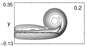
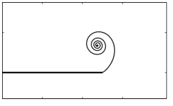
Figure 5: *

(for caption see next page)

Figure 6: Vorticity, streaklines, and streamlines, for $Re=500$ at a sequence of times, $t=0.005,0.02,0.04,0.1,0.2,0.5,1.0,3.0,5.0$, as indicated. The vorticity contour levels are $\omega=\pm 2^{[-5:12]}$. The stream function levels are $\psi=[-1:0.05:1]$ for $t\leq 1$ (previous page) and $\psi=[-1:0.1:1]$ for $t=3,5$ (this page).

The driving far field flow $\boldsymbol{u}_{\infty}$ is the potential flow moving upwards past and around the plate. Initially, the flow generates a boundary layer of positive vorticity along both the upstream and downstream sides of the right half-plate. Upstream vorticity is convected downstream, concentrating near the tip as a vortex that grows in time. The vortex entrains nearby vorticity, while vorticity further away is swept from the vortex towards the axis, thus depleting the region in between. As a result, the leading vorticity, which initially is connected to the downstream boundary layer, begins to separate from it. At some time between t=0.2 and 0.5, the positive vorticity in the leading vortex has completely separated from the positive boundary layer vorticity, resulting in a more clearly defined starting vortex.

The leading vortex induces a region of recirculating flow that can be seen in the corresponding streamlines. The region of recirculating flow forms immediately after the motion begins. The fluid within this region, below the center of rotation, flows in direction opposite to the starting flow, and generates negative vorticity attached to the wall. In the computations, the negative vorticity is observed already after a few timesteps. It is barely visible in figure 6, at t=0.005, but grows in time and is clearly discernible by the grey contours at later times. The negative vorticity region grows horizontally along the plate, away from the starting vortex, until it reaches the axis at $t\approx 0.113$, as will be shown later. At the same time, the negative vorticity region is stretched and entrained into the leading vortex. As the negative vorticity layer thickens, the positive boundary layer vorticity above it diffuses, until eventually, after $t=1.0$ shown here, all downstream boundary layer vorticity is negative. Around time $t=3$, the positive vorticity in the starting vortex has reached the axis of symmetry, $x=0$. It diffuses out of the recirculation region, so that at $t=5$, much vorticity is outside the enclosing streamline and moves upwards away from the plate. The results at the larger times presented here are in good agreement with results shown by [Koumoutsakos and Shiels (1996)].

Figure 7: Closeup of vorticity contours near the plate tip, for $Re=500$, $p=0$, at (a) $t=0.0002$, (b) $t=0.0016$, (c) $t=0.008$ and (d) $t=0.1$. Vorticity contour levels are $\pm 2^{[-8:15]}$.

The streaklines, shown in the middle column of figure 6, are obtained by releasing a particle at a point near the tip at each timestep, and computing its evolution with the fluid velocity. At a given time, the figure shows the position of all particles at that time that were released previously. The streakline plots thus mimic what one would observe in a laboratory experiment if dye were continously released at a point near the tip. Each released particle circulates around the vortex center. Particles that have been released earlier travel closer to the center and thus, the resulting streakline has a spiral shape. The spiral tightens near the center and the number of spiral turns increase in time. The maximum vorticity near the tip of the plate is convected with the particles along the streakline, and diffuses. Thus the streakline is a good indicator of the centerline of the separated shear layer, but not of the overall vortical region, or of the recirculation region, both which extend beyond the region occupied by the spiral. At the times shown, the spiral center is a good indicator of the vorticity maximum in the vortex core, and of the center of fluid rotation.

The streamlines, in the right column, show the region of recirculating flow. This region is enclosed by the $\psi=0$ streamline, which leaves the tip of the plate and reattaches on the downstream side, at a short distance behind the vortex. As the recirculation region grows, the enclosing streamline $\psi=0$ first reaches the axis, between time $t=0.1$ and $0.2$, and then continues to move up along the centerline, $x=0$. It then forms the familiar rounded symmetric recirculation bubble downstream of the plate, as observed experimentally and computationally, before the flow looses its symmetry at later times (see, eg, van Dyke 1982, figure 64, and Koumoutsakos & Shiels 1996, figure 18).

Figure 8: Wall vorticity (a) $\omega_{+}(x)$, and (b) $\omega_{-}(x)$, on the upstream and downstream sides of the plate, respectively, vs. $x$, at a sequence of times $t=$0.0002, 0.0004, 0.001, 0.002, 0.005, 0.01, 0.02, 0.04, 0.08, 0.2, 0.5, 1, 3, 5, for $Re=500$. The vorticity decreases in magnitude as time increases.

Figure 9: Vorticity $t=0.04$ along the lines $x$=0.4, 0.425, 0.45 and 0.475, as functions of $y$. The arrows indicate increasing values of $x$.

Figure 7 shows a closeup of the vorticity contours near the tip of the plate, plotted as the black and grey solid contour lines. It also shows two of the flow streamlines as dashed curves. One is the $\psi=0$ streamline enclosing the region of recirculating flow, the other is a closed streamline near the center of rotation. Figure 7(a) shows that very early, at $t=0.0002$, the negative vorticity region is already well-formed, all along the wall inside the recirculation region. Positive vorticity has begun to concentrate downstream, near the tip of the plate, but it does not yet have a local vorticity maximum that could identify a vortex core. On the other hand, the recirculation region is well-formed and has a well-defined center of rotation. Thus, this early on, the center of rotation does not agree with a maximum in the core vorticity. Figure 7(b), which plots the solution a little later, at $t=0.0016$, shows a local vorticity maximum emerging in the center of the leading vortex. This local maximum remains well defined and grows in time, as shown in figures 7(c,d). As time increases, the center of rotation and the position of the vorticity maximum are in better agreement. Figure 7(d) also shows the entrainment of the negative vorticity by the leading vortex.

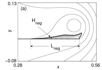
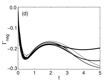
Figure 10: Quantifiers of negative vorticity region. (a) Negative vorticity contours and streamlines at $t=0.04$, showing definition of length $L_{neg}$ and thickness $H_{neg}$. (b) Length $L_{neg}$ vs. t. (c) Thickness $H_{neg}$ vs. $t$. (d) Integral negative vorticity $\Gamma_{neg}$ vs. $t$. Figures (b,c,d) show results for $Re=250,500,1000,2000$, as indicated in the legend in (b).

Figures 9-10 show details of the vorticity profiles on and near the plate. Figure 9(a) plots the wall vorticity $\omega_{+}$ on the upstream side of the plate at a sequence of times. The vorticity is initially unbounded at the plate tip, zero at the axis, and positive, increasing, in between. As time increases, it remains positive but decreases in magnitude. Figure 9(b) plots the wall vorticity $\omega_{-}$ on the downstream side of the plate. At $t=0+$, the vorticity is also positive everywhere, but negative unbounded at the tip. The interval along the plate in which the vorticity is negative grows, and the maximal magnitude decreases. The wall vorticity values are responsible for the drag forces normal to the wall parallel to the background flow, presented later in §4.5. Figure 9 plots the vorticity at a fixed time t=0.04, along four vertical lines crossing the region of negative vorticity, $x=0.4$, 0.425, 0.45, 0.475, as a function of $y$. The arrows indicate the direction of increasing $x$. The vorticity is positive on the upstream side of the plate ($y<0$), and negative downstream ($y>0$). As $x$ increases towards the tip, the wall vorticity and their gradients $\partial\omega/\partial y$ increase in magnitude. The wall vorticity gradients are responsible for the lift forces parallel to the wall, normal to the background flow, presented in §4.5.

Figure 10 gives more information on the region of negative vorticity. It plots its length $L_{neg}$ and a characteristic thickness $H_{neg}$, both of which are illustrated in figure 10(a), and the integral negative vorticity $\Gamma_{neg}$. For later reference, results are plotted for various Reynolds numbers, as indicated in the legend in figure 10(b). The length $L_{neg}$, plotted in figure 10(b), is also the length of the recirculation region. It increases until it reaches $L_{neg}=0.5$, which is when the recirculation region reaches the axis. For $Re=500$, this occurs at $t\approx 0.113$, for larger $Re$, it occurs sooner. After this time, negative vorticity covers all of the downstream plate wall. The thickness $H_{neg}$, plotted in figure 10(c), is chosen to be the thickness of the negative vorticity region at $x=0.4$. It increases initially, reaches a maximum, and then decreases again as the negative vorticity is entrained by the leading vortex. Larger Reynolds number flows have thicker regions of negative vorticity. The behaviour at places other than $x=0.4$ is similar. The integral negative vorticity in the right hand plane,

$$\Gamma_{neg}=\int_{\omega<0\atop x\geq 0}\omega\,dA~{},$$ (16)

is plotted in figure 10(d). Remarkably, even though the layer thickness $H_{neg}$ depends heavily on $Re$, its integral circulation is practically independent of $Re$, at least until about $t=3$. After that, diffusion causes the integral negative vorticity to decrease in magnitude, with larger decrease for lower $Re$.

4.2 Dependence on $Re$

Figure 11: Vorticity, streak lines and streamlines at $t$=1 for $Re$=250, 500, 1000 and 2000. Vorticity contour levels are $\pm 2^{[-5:12]}$, and streamlines contour levels are $[-1:0.1:1]$.

Figure 10 shows the dependence of vorticity contours, streamlines and streaklines at a fixed time $t=1$ on Reynolds number, for $Re\in[250,2000]$. As $Re$ increases, the vorticity contours show well-known features: the wall boundary layer thickness decreases; the separated shear layer thickness decreases, and its spiral roll-up becomes more evident; the thickness of the negative vorticity region decreases, as already seen in figure 9(c). For larger $Re$, the separated vorticity is supported in a smaller, more compact region.

Some dependence on $Re$ is also observed in the spiral streaklines. Most noticeably, the spiral roll-up near the center is tighter for larger $Re$, and there are more spiral turns. The spiral size does not depend much on $Re$, and is, in particular, not a good indicator of the size of the vortex structure. The size of the recirculation region does not depend much on $Re$ either. The streamline density within the vortex increases with $Re$, indicating larger gradients, that is, larger fluid velocities.

A measure of the boundary layer thickness is given by the thickness $\delta$ of the positive vorticity region on the upstream side of the plate, at $x=0.2$, plotted in figure 12. Here, $\delta$ is the thickness of the region with $\omega\geq 2^{-5}$. The figure shows that when plotted against $t/Re$, the results for all $Re$ collapse onto a line of slope $1/2$, and thus

$$\delta\sim(t/Re)^{1/2}.$$ (17)

asymptotically, as $t\to 0$. This is in agreement with results for self-similar flow past infinite plates. The thickness at other values of $x$ is qualitatively similar.

Figure 12: Boundary layer thickness $\delta$ vs. $t/Re$. Results are shown for $Re$=250, 500, 1000 and 2000, as indicated.

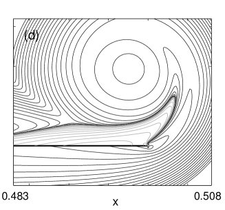
Figure 13: Closeup of vorticity contours near the plate tip, at $t=0.005$, with (a) $Re=250$, (b) $Re=500$, (c) $Re=1000$, (d) $Re=2000$. Vorticity contour levels are $\pm 2^{[-8:15]}$.

Figure 13 shows a closeup of the vorticity at a fixed early time, for different Reynolds numbers. With low $Re$, as in figure 13(a), the vorticity has not yet formed a local maximum away from the tip and the negative vorticity is not yet entrained past the tip. For larger $Re$, the core vorticity increases, the negative vorticity region lengthens and rolls up around the spiral. These features at a fixed time, as $Re$ increases, are similar to the features observed with fixed $Re$, as time increases (see figure 6), up to scale, which is as expected at early times in which the presence of a length scale is not yet noticeable.

4.3 Core vorticity and trajectory

Figure 14: Core vorticity and trajectory, for $Re=250,500,1000,2000$ as indicated. (a) Core vorticity $\omega_{c}$ vs. $t$. (b) Core vorticity $\omega_{c}$ vs. scaled time $t/Re$. (c,d) Vertical core position $y_{c}$ vs. $t$. (e,f) Horizontal core displacement $x_{c}-0.5$ from edge. The dashed lines have the indicated slopes.

The core position and vorticity are defined as the coordinates $(x_{c},y_{c})$ and vorticity $\omega_{c}$ at the local vorticity maximum in the leading vortex (see figure 2d). They are defined only after this local maximum away from the tip of the plate has formed. As seen in figure 13, this occurs earlier for higher $Re$. This section investigates their scaling behaviour and dependence on $Re$. We note that alternatively, the core position can be defined as the center of rotation, which exists at all times, but this option is not explored here.

Figure 14 plots the core coordinates and vorticity computed for all $Re$, as indicated in the legend in figure 14(a), and all values of $h$ used, as given in table 2. Thus, each subplot in figure 14 shows results for about 20 different time series, computed with different $Re$ and resolutions. Figure 14(a) plots the values of $\omega_{c}$ vs. t. The values show remarkably little dependence on the resolution: only for the largest Reynolds numbers do we see small jumps in the values of $\omega_{c}$ as $h$ is doubled. The values $\omega_{c}$ appear linear in the logarithmic scale, with a vertical shift between different $Re$. By plotting the results versus $t/Re$, in figure 14(b), all the data collapse onto one curve, and agree for over more than 5 decades in time with the approximation,

$$\omega_{c}\approx 0.335{\left(Re\over t\right)}^{3/4}.$$ (18)

Thus, at any fixed time, the core vorticity increases as $Re^{3/4}$. For fixed $Re$, it decreases in time as $t^{-3/4}$. We do not know of an analytical result that explains this observation.

Figures 14(c,d) plot the vertical displacement $y_{c}$ of the vortex core from the plate, on a linear and a logarithmic scale respectively, versus t. Here again, the values for all $Re$ and all resolutions computed collapse onto one curve, with no apparent dependence on $h$, and only a small dependence on $Re$ visible at later times. The data for all $Re$ scales for about 4 decades as

$$y_{c}\approx 0.37t^{2/3}$$ (19)

with deviations from this line visible after approximately $t=1$. This scaling agrees with the self-similar inviscid spiral roll-up of semi-infinite free vortex sheets, or of separated vortex sheets at the edge of a semi-infinite plate (Kaden 1931, Pullin 1978).

Figure 14(e) plots the horizontal displacement $x_{c}-0.5$ of the vortex core from the plate, on a linear scale. Figure 14(f) plots the absolute value on a logarithmic scale. These values are an order of magnitude smaller than those of $y_{c}$, and less well resolved, with the dependence on $h$ more visible. To within the available resolution, the results depend little on $Re$. The linear scale shows that $x_{c}-0.5$ is initially negative. Up to about $t=2$, the symmetric vortices at each end of the plate more slightly inward, as they would in the self-similar inviscid case. After that time they begin moving outwards again, with $x_{c}>0.5$ at the final time computed, $t=5$. The logarithmic scale shows that until about $t=1$, $x_{c}$ also satisfies the self-similar inviscid scaling, with

$$x_{c}-0.5\approx-0.1t^{2/3}~{}.$$ (20)

Figure 15: Comparison of vortex core coordinate with experimental data of Pullin & Perry (1980). (a) Vertical displacement $y_{c}$. (b) Horizontal displacement $x_{c}$. The computed data for all Reynolds number and the experimental data is shown, as indicated in the legend. The vertical bars through the experimental data are the error bars indicated in P&P.

The closest data on viscous flow at early times available for comparison in the literature are the experimental measurements of Pullin & Perry (1980), who measured vortex core positions in flow past wedges and compared them to similarity theory. Figure 15 reproduces their results for the smallest wedge considered, of wedge angle $\beta=5^{o}$, together with our computed results. The experimental data span an early time interval $t\in[0,0.3]$. The vertical displacement $y_{c}$ is in quite good quantitative agreement with the computed values. The horizontal displacement $x_{c}$ overlaps with the present better resolved values at the lower Reynolds numbers, except for the last two data points. The experimental data was obtained at larger Reynolds number of $Re\approx 6000$, but the data is expected to be practically independent of $Re$, as is clearly the case for the values of $y_{c}$. We cannot explain the deviation of the computation from the last two experimental data points in figure 15(b).

Figure 16: Scaled vorticity $\omega/Re^{0.75}$ (left column) and dissipation $\Delta\omega/Re$ (right column) at $t=1$, for $Re$=250, 500, 1000 and 2000, from top to bottom. The colorbar is the same for all values of $Re$, and shown for highest $Re$ only.

With knowledge of the core vorticity scaling, we now plot scaled vorticity, as well as dissipation. Figure 16 shows color coded contours of the scaled fluid vorticity, $\omega/Re^{3/4}$, at $t=1$, for the indicated values of $Re$ (left column), and of the corresponding dissipation $\Delta\omega/Re$ (right column). For clarity, we note that the plots consist of equally spaced contour curves of $A\tanh(q/A)$, for a chosen value of $A$ below the true maximum, where $q$ is either the scaled vorticity or dissipation. As a result, contours of arbitrarily large levels can be shown. Also as a result, the values of the quantity $q$ shown in the attached colorbars are not equally spaced in the color level.

At this time, the vorticity attached to the upper plate wall is all negative, and all remaining vorticity is positive. The vorticity contours show the decrease of boundary and shear layer thicknesses, and the increasingly visible spiral shear layer roll-up as $Re$ increases. In a crossection at any point through the shear layer, the vorticity is largest in the middle of the layer, and decreases to local minima in between different spiral turns. We note that at this rather late time, the vorticity maximum only approximately satisfies the scaling $\omega_{c}\sim Re^{3/4}$, and the scaled values plotted in the figure decrease from 0.359 to 0.250.

The dissipation plot indicates the magnitude of viscous diffusion in the flow. The dissipation at the vortex core, where the vorticity has a maximum, is negative, which causes the maximum vorticity to decrease. The largest absolute values at the core increase as $Re$ increases, from 16.16 to 54.96, in a manner consistent with the scaling

$${\Delta\omega\over Re}\sim Re^{3/4}~{}.$$ (21)

Across each of the spiral shear layer turns the dissipation changes sign twice. It is positive at the local vorticity minima in between spiral turns, causing these minimum values to increase, and it is negative at the local maxima in the middle of the layer, causing these maxima to decrease. As a result, the spiral turns are more clearly visible in the dissipation plots than in the vorticity contours. The dissipation is largest in magnitude near the tip of the plate, where it reaches values well above 200.

4.4 Shed vortex circulation

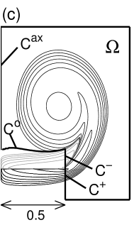
Figure 17: Sketch defining the domain $\Omega$ and portions $C^{+},C^{-},C^{s},C^{o},C^{ax}$ of its boundary with nonzero circulation flux.

4.4.1 Definitions

One of our main interest in performing the present simulations was to obtain circulation shedding rates for the viscous flow, for which little data is available in the literature. We are interested in resolving the shed circulation over large time scales, including early times. However, at early times the vorticity in the leading vortex is not clearly distinguished from the boundary layer vorticity. Here, we define the shed circulation to be

$$\Gamma=\int_{\Omega(t)}\omega\,dA~{},$$ (22)

where the region $\Omega(t)$ is defined in figure 17. The circulation is normalized by $UL$.

The definition of $\Omega$ is defined slightly differently in different time-regimes of the flow, with continuous transitions between them. At early times, when the region of negative vorticity has not yet been entrained past the vertical line $x=0.5$, we follow the sketch in figure 17(a). On the upstream side ($y<0$), the region $\Omega$ is bounded by the vertical line through the tip, $C^{+}$. On the downstream side ($y>0$), it is bounded by the zero vorticity contour $C^{o}$ that separates negative from positive vorticity, and by a slant line $C^{s}$ through points of high curvature visible in the vorticity contours. That is, the region $\Omega$ is defined to include all vorticity to the right of the tip, to exclude the negative boundary layer vorticity, and is limited on the left by the slant line. Figure 17(b) shows the vorticity at intermediate times, when the negative vorticity on the downstream side has been entrained past the vertical line $x=0.5$. Here we include all vorticity, positive or negative, to the right of the vertical line through the tip, which introduces a vertical piece of boundary $C^{-}$ above the plate. Figure 17(c) shows the vorticity at later times, when all the positive boundary layer vorticity on the downstream wall has diffused and effectively vanished. At this time the vortex is bounded on the left not by the slant line, but by the axis $C^{ax}$. Each subplot in figure 17 shows a typical length scale, indicating that the three regimes in time span three decades of length scales in space.

In order to determine the effect of viscous diffusion relative to inviscid convection of vorticity into $\Omega$, and also to determine the suitability of the definition above, we consider shedding rates of vorticity through the various components of the boundary of $\Omega$. By applying the Transport Theorem, the Navier Stokes Equations, and the Divergence Theorem, one finds that

$$\begin{split}\frac{d\Gamma}{dt}&=\frac{d}{dt}\int_{\Omega(t)}\omega(\boldsymbol{x},t)\,dA\\ &=\int_{\Omega(t)}\frac{\partial\omega}{\partial t}\,dA+\int_{\partial\Omega}\omega(\boldsymbol{u}_{bd}\cdot\boldsymbol{n})\,ds\\ &=\int_{\Omega(t)}\left[-(\boldsymbol{u}\cdot\nabla)\omega+{1\over Re}\Delta\omega\right]\,dA+\int_{\partial\Omega}\omega(\boldsymbol{u}_{bd}\cdot\boldsymbol{n})\,ds\\ &=\int_{\partial\Omega(t)}\left[-\omega\boldsymbol{u}\cdot\boldsymbol{n}+{1\over Re}\nabla\omega\cdot\boldsymbol{n}+\omega(\boldsymbol{u}_{bd}\cdot\boldsymbol{n})\right]\,ds=\frac{d\Gamma_{c}}{dt}+\frac{d\Gamma_{d}}{dt}+\frac{d\Gamma_{m}}{dt}\end{split}$$ (23)

where $\boldsymbol{n}$ is the outward normal, and $\boldsymbol{u}_{bd}$ is the velocity of the boundary. That is, across each piece of the boundary there is a contribution to the vorticity due to convection, diffusion, and the moving boundary. We denote these components by subscripts $c$, $d$, and $m$ respectively. Notice that the only moving boundary portions are $C^{o}$ and $C^{s}$, and the latter has no nonzero vorticity moving with it or convecting through it. Similarly, there is no convection of vorticity through $C^{ax}$. Thus the nonzero contributions to the circulation shedding rate are the 9 components

$$\frac{d\Gamma^{+}_{c}}{dt}~{},\quad\frac{d\Gamma^{-}_{c}}{dt}~{},\quad\frac{d\Gamma^{s}_{c}}{dt}~{},\quad\frac{d\Gamma^{+}_{d}}{dt}~{},\quad\frac{d\Gamma^{-}_{d}}{dt}~{},\quad\frac{d\Gamma^{o}_{d}}{dt}~{},\quad\frac{d\Gamma^{s}_{d}}{dt}~{},\quad\frac{d\Gamma^{ax}_{d}}{dt}~{},\quad\frac{d\Gamma^{s}_{m}}{dt}$$

where the superscript refers to the portion of the boundary, and the subscript refers to the component of the shedding rate. For conciseness, we combine two of the viscous components into one:

$$\frac{d\Gamma^{-}_{d}}{dt}+\frac{d\Gamma^{o}_{d}}{dt}\rightarrow\frac{d\Gamma^{-}_{d}}{dt}~{}.$$

Below, we first investigate the 8 circulation shedding rates for $Re=500$, and then determine dependence on $Re$.

4.4.2 $Re=500$

                 

Figure 18: Circulation and shedding rates for $Re=500$. (a) Circulation $\Gamma(t)$, linear scale. (b) Circulation $\Gamma(t)$, logarithmic scale. (c) Components $d\Gamma^{+}_{c}(t)/dt$, $d\Gamma^{+}_{d}(t)/dt$, $d\Gamma^{-}_{d}(t)/dt$, $d\Gamma/dt$, on a logarithmic scale (d) Components $d\Gamma^{s}_{c}(t)/dt$, $d\Gamma^{s}_{d}(t)/dt$, $d\Gamma^{s}_{m}(t)/dt$.

Figures 18(a,b) plot the shed circulation computed using the above definition for Re=500. The logarithmic scale in figure 17(b) shows that the circulation satisfies the scaling behaviour predicted by inviscid similarity theory (Pullin 1978) surprisingly well, $\Gamma(t)\sim t^{1/3}~{}.$ Moreover, it shows that the circulation is resolved over more than 4 decades in time. Finally, we note that just as the data for $\omega_{c}$ and $y_{c}$, the circulation data shows remarkable independence of the meshsize used in the computation. Even though the figure plots the results for all meshsizes and time intervals given in table 2, the data is an almost continuous function of the meshsize.

Figures 18(c,d) show some of the circulation flux components. The largest flux into the region is the convective component through the vertical $C^{+}$ on the upstream side of the plate, $d\Gamma_{c}^{+}/dt$, shown as the thickest curve in figure 18(c). It is larger than $d\Gamma/dt$, shown as the dashed curve. The viscous flux components are negative and reduce the total circulation. Of these, largest in magnitude is the viscous flux through $C^{-}\cup C^{o}$, $d\Gamma_{d}^{-}/dt$, shown as the curve of medium thickness. We conclude that $d\Gamma_{c}^{+}/dt$ is most significant, but the contribution to the total flux due to viscous diffusion is nonnegligible.

Figure 18(d) shows the three flux components through the slant line. To note is, first, that these are much smaller than the the largest components shown in figure 18(c) and do not contribute significantly to the circulation, and second, that they vanish quickly and are negligibly small after about $t=0.005$. Thus, not much vorticity leaves or enters through the slant line, making it a reasonable left boundary to the leading vortex.

4.4.3 Dependence on $Re$

Figure 19: Dependence of circulation shedding rate components on Re, for $Re=250,500,1000,2000$. (a) $d\Gamma_{d}^{ax}/dt$ (b) $d\Gamma_{c}^{-}/dt$, (c) $d\Gamma_{c}^{+}/dt$, (d) $d\Gamma^{-}_{d}/dt$, vs. $t$.

In order to determine the dependence of the shed circulation on $Re$, figure 19 plots several circulation flux components for $Re=250,500,1000,2000$. Figure 19(a) shows that the viscous loss of vorticity through the axis depends clearly on $Re$, but is comparatively very small. Similarly, the convective component through the vertical $C^{-}$ on the downstream side of the plate, shown in figure 19(b), depends on $Re$ but is small. The largest component, the convective component through the vertical $C^{+}$ on the upstream side of the plate, shown in figure 19(c), is completely independent of $Re$. The next largest component, the viscous component of vorticity diffusion through $C^{-}\cup C^{o}$, shown in figure 19(d), appears to be quite independent of $Re$ at early times, based on the results for $Re=250,500,1000$. For $Re=2000$, the results are not fully resolved, due to the difficulty in resolving the large vorticity gradients present near the tip of the plate.

We conclude from figure 19 that the flux is essentially independent of $Re$. The convective flux is clearly so, and the dominant diffusive flux, even though it is large, is largely independent on $Re$. We attribute the latter to the fact that as $Re$ increases, vorticity gradients increase, but are offset by the $1/Re$ factor in the diffusive term of equation (4.8),

$${1\over Re}\int\nabla\omega\cdot\boldsymbol{n}\,ds\,.$$ (24)

Figure 20 plots the circulation $\Gamma(t)$ for $Re=250,500,1000,2000$. Consistent with the conclusions based on figure 19, the circulation is basically independent on $Re$ at early times. As time increases, differences between $Re$ increase slightly. The largest difference over the range of $Re$ considered here occurs at the last time computed, $t=5$, and is less than 5% of the circulation at that time. The logarithmic plot in figure 20(b) shows that all 20 time series computed with different values of $Re$ and meshsizes collapse onto one curve, which is well approximated by

$$\Gamma(t)\approx 2t^{1/3}~{}\text{ as }~{}t\to 0~{}.$$ (25)

Figure 20: Dependence of total shed circulation $\Gamma(t)$ on $Re$, for $Re=250,500,1000,2000$, as indicated. (a) linear scale, (b) logarithmic scale.

4.5 Vortex forces

The vorticity profiles on the plate wall induce drag and lift forces. Here we compute the drag and lift, $F_{D}$ and $F_{L}$, defined to be total force parallel and normal to the background flow, in the right half of the plate only. They are given by (Eldredge 2007)

$$F_{D}(t)={2\over Re}\int_{0}^{1/2}\left[\omega_{+}(x,0,t)+\omega_{-}(x,0,t)\right]\,dx~{},$$ (26a)

$$F_{L}(t)={2\over Re}\int_{0}^{1/2}x\left[{\partial\omega_{+}\over\partial y}(x,0,t)+{\partial\omega_{-}\over\partial y}(x,0,t)\right]dx~{},$$ (26b)

where all forces are normalized by ${1\over 2}\rho U^{2}L$. By symmetry, the overall lift force acting on the whole plate is zero, and the total drag is $2F_{D}$.

Figure 21: Forces (a) $F_{L}$ and (b) $F_{D}$ for $Re=1000$, computed with the indicated values of $h$. For comparison, (b) includes the data by Koumoutsakos & Shiels (1996, denoted by KS).

Computing the forces using formulation (26b) is sensitive to discretization errors, since the formulation depends on values of the vorticity and its derivatives on the plate wall. These values are large and difficult to compute accurately, specially near the tip. To illustrate, figure 21 plots the computed lift and drag for $Re=1000$ for various values of $h$ used and shows that the convergence in $h$ is slow. An alternative formulation for the drag force is used by [Koumoutsakos and Shiels (1996)] (KS), who compute drag as the time derivative of an area integral, see their equations (40-41). The value of $F_{D}$ given by (26bb) corresponds to the variable $c_{D}$ plotted in KS in their figure 13. Figure 21(b) in this paper compares the drag computed here with the values computed by KS, for $Re=1000$. The figure shows that the values are in fairly good agreement, although differences exist, mainly in the decay rate at early times.

Figures 22(a,b) plot the lift and drag force on a logarithmic scale, for all Reynolds numbers computed here, and for all values of $h$ used. They show that the results at early times collapse quite well onto a common curve. Figure 22(a) plots the lift force versus a scaled time $Re\cdot t$. In these variables, the data at early times collapses onto a curve that decreases in time and in $Re$ approximately as

$$F_{L}(t)\approx(Re\cdot t)^{-{1/2}}~{}.$$ (27)

The drag, on the other hand, plotted in figure 22(b) versus time $t$, appears to be almost independent of $Re$, and is approximately given by

$$F_{D}(t)\approx 6t^{-1/2}~{}.$$ (28)

These results suggest that at a fixed time, the lift decays significantly faster, as $1/Re^{1/2}$, than the drag, which remains almost constant in $Re$ for early times. In view of equation (26b), this in turn indicates that the wall vorticity grows as $Re^{1/2}$, while the wall vorticity gradients grow faster, almost linearly in $Re$. At later times the drag force decreases as $Re$ increases, consistent with the results shown by Dennis et al (1993) and by KS.

Figure 22: (a) Lift force vs. $Re\cdot t$. (b) Drag force vs. $t$. Results are shown for $Re=250,500,1000,2000$, as indicated in the legend in figure (a). The dashed lines have the indicated slopes.

5 Summary

Viscous flow past a flat plate of zero thickness which is impulsively started in direction normal to itself is studied using highly resolved numerical simulations for a range of Reynolds numbers $Re\in[250,2000]$. Several features of the flow are revealed by the computations.

The evolution of the vorticity profiles shows the growth of the leading vortex emanating from the boundary layer during the early starting flow, the growth of the region of opposite-signed vorticity on the plate, and the evolution of the plate vorticity and vorticity gradients. Increasing Reynolds numbers leads to thinning of boundary layer and shear layer thicknesses, and to increasingly many and tighter spiral streakline turns in the vortex center.

Scaling behaviours that capture the dependence on time and on $Re$ were found for several quantities in the flow, over several decades in time. Some quantities clearly depend strongly on $Re$, such as the core vorticity, the boundary layer thickness, and the lift force over the half-plate, with

$$\omega_{c}(t)\approx 0.335\Big{(}{\tiny Re\over t}\Big{)}^{3/4}~{},\quad\delta(t)\sim\Big{(}{\tiny t\over Re}\Big{)}^{1/2}~{},\quad F_{L}(t)\approx(Re\cdot t)^{-1/2}~{},$$ (29a)

all as $$t\to 0 Re$$. Other quantities of the early starting flow are largely independent on , such as the core trajectory, the shed circulation, the integral negative vorticity, and the drag force over the half-plate, with

$$y_{c}(t) \approx 0.37t^{2/3}~{},\quad x_{c}(t)-0.5\approx-0.1t^{2/3}~{},\quad$$ (29b)

$$\Gamma(t) \approx 2t^{1/3}~{},\qquad F_{D}(t)\sim t^{-1/2}~{}.$$ (29c)

The scaling for $x_{c}$, $y_{c}$ and $\Gamma$ are in excellent agreement with the inviscid scaling laws for self-similar roll-up.

One of the main contributions is to define and compute the viscous shed circulation, specially at early times, when the shed vorticity is not clearly separated from the boundary layer vorticity. Our definition is validated by plots of the circulation shedding rates across various portions of the boundary defining the shed vorticity, which show that practically no vorticity enters or leaves the boundary by convection except near the tip, where it is convected into the vortex by the separating boundary layers. With this definition, the shed circulation satisfies the self-similar scaling laws for more than three decades in time.

The presentation of several components of the circulation shedding rate gives insight into the effect of viscosity on the total circulation. The largest component is the gain of circulation due to convection of vorticity from the upstream boundary layer into the leading vortex. This component is highly independent of the Reynolds number. It is offset by loss of circulation due to viscous diffusion of vorticity out of the boundary, which is of opposite sign but also significant in magnitude. Interestingly, this diffusive component also depends little on $Re$ at early times, consistent with the fact that the overall shed circulation is basically independent of $Re$ at these times. This observation suggests that that as $Re$ increases, vorticity gradients responsible for viscous diffusion grow in such a way that the quotient $\nabla\omega/Re$ changes little. We conclude that the effect of viscous diffusion on the overall shed circulation is significant, but its contribution depends little on the value of $Re$.

Appendix

In this appendix we compare the scaling laws observed in this paper using two alternate nondimensionalizations. For clarity, in this appendix only, let all variables without a hat or double hat, such as $x,t,\Gamma,\omega,F_{D}$, denote the original dimensional variables. Let all variables with one hat denote variables nondimensionalized by length and time scales $L$ and $L/U$. For example,

$$\widehat{x}={x\over L}~{},\quad\widehat{t}={Ut\over L}~{},\quad\widehat{\Gamma}={\Gamma\over LU}~{},\quad\widehat{\omega}={L\omega\over U}~{},\quad\widehat{F_{D}}={F_{\tiny D}\over{1\over 2}LU^{2}}~{}.$$

These are the nondimensional variables used throughout this paper, where for simplicity, the hats were dropped. Let all variables with two hats denote variables nondimensionalized by length and time scales $\nu/U$ and $\nu/U^{2}$. For example,

$$\widehat{\widehat{x}}={Ux\over\nu}~{},\quad\widehat{\widehat{t}}={U^{2}t\over\nu}~{},\quad\widehat{\widehat{\Gamma}}={\Gamma\over\nu}~{},\quad\widehat{\widehat{\omega}}={\nu\omega\over U^{2}}~{},\quad\widehat{\widehat{F_{D}}}={F_{D}\over{1\over 2}\nu U}~{}.$$

It follows that

$$\widehat{\widehat{x}}=Re\cdot\widehat{x}~{},\quad\widehat{\widehat{t}}=Re\cdot\widehat{t}~{},\quad\widehat{\widehat{\Gamma}}=Re\cdot\widehat{\Gamma}~{},\quad\widehat{\widehat{\omega}}={\widehat{\omega}\over Re}~{},\quad\widehat{\widehat{F_{D}}}=Re\cdot\widehat{F_{D}}~{}.$$

Therefore, the observed scaling laws, given in equations (29) in the single-hat variables, are given in the double-hat variables as

$$\widehat{\widehat{\omega}}_{c}\approx\,0.335\,{Re^{1/2}~{}\widehat{\widehat{t}}{~{}}^{-{3/4}}}~{},$$

$$\widehat{\widehat{\delta}}\sim\widehat{\widehat{t}}{}^{~{}{1/2}}~{},$$

$$\widehat{\widehat{F_{L}}}\approx\,Re\cdot\widehat{\widehat{t}}{}^{~{}-{1/2}}~{},$$

$$\widehat{\widehat{y}}_{c}\approx\,0.37\,Re^{1/3}~{}\widehat{\widehat{t}}{}^{~{}{2/3}}~{},$$

$$\widehat{\widehat{x_{c}}}\approx\,-0.1\,Re^{1/3}~{}\widehat{\widehat{t}}{}^{~{}{2/3}}~{},$$

$$\widehat{\widehat{\Gamma}}\approx\,2\,Re^{2/3}~{}\widehat{\widehat{t}}{}^{~{}{1/3}}~{},$$

$$\widehat{\widehat{F_{D}}}\sim(Re/\,\widehat{\widehat{t}}~{})^{{1/2}}~{},$$

all as $\widehat{\widehat{t}}\to 0$. Notice that of all these, one variable, namely the boundary layer thickness $\widehat{\widehat{\delta}}$, scales as a function of $\widehat{\widehat{t}}$ independent of the value of $Re$. One may therefore suggest that the double-hat nondimensionalization is more natural for this variable. Using the same argument one may say that the single-hat nondimensionalization is more natural to describe the vortex coordinates and circulation, as in equations (5.1bc). The essence is that the variables depend on $L,U,\nu$ as described by either equations (A.3) or (5.1).

References

- [Alben and Shelley (2008)] S. Alben and M. J. Shelley, 2008, Flapping States of a Flag in an Inviscid Fluid: Bistability and the Transition to Chaos, Physical Review Letters, 100, 074301.
- [Cortelezzi and Leonard (1993)] L. Cortelezzi and A. Leonard, 1993, Point vortex model of the undsteady separated flow past a semi-infinted plate with transverse motion, Fluid Dyn. Res., 11, 264-295.
- [Dennis et al (1993)] S. C. R. Dennis, W. Qiang, M. Coutanceau and J.-L. Launay, 1993, Viscous flow normal to a flat plate at moderate Reynolds numbers J. Fluid Mech., 248, 605-635.
- [E and Liu (1996)] W. E and J. G. Liu, 1996, Essentially compact schemes for unsteady viscous incompressible flows, J. Comput. Phys., 126, 122-138.
- [Eldredge (2007)] J. D. Eldredge, 2007, Numerical simulation of the fluid dynamics of 2D rigid body motion with the vortex particle method, J. Comput. Phys., 221, 626-648.
- [Eldredge and Wang (2010)] J. D. Eldredge and C. Wang, 2010 High-fidelity simulations and low-order modeling of a rapidly pitching plate, AIAA, 2010-4281, 1–19.
- [Fletcher (1991)] C. A. J. Fletcher, 1991, Computational techniques for fluid dynamics, Vol.1, Springer Verlag, New York.
- [Hudson and Dennis (1985)] J. D. Hudson and S. C. R. Dennis, 1985, The flow of a viscous incompressible fluid past a normal flat plate at low and intermediate Reynolds numbers: the wake, J. Fluid Mech., 160, 369–383.
- [Johnston (1999)] H. E. Johnston, 1999, Efficient computation of viscous incompressible flow, PhD. thesis, University of Maryland.
- [Jones 2003] M. Jones, 2003, The separated flow of an inviscid fluid around a moving flat plate, J. Fluid Mech., 496, 405–441.
- [Jones and Shelley (2005)] M. A. Jones and M. J. Shelley, 2005, Falling cards, J. Fluid Mech., 540, 393-425.
- [Kaden (1931)] H. Kaden, 1931, Aufwicklung einer unstabilen Unstetigkeitsfläche, Ing. Arch 2, 140 (English trans. R.A.Lib.Trans. no.403).
- [Koumoutsakos and Shiels (1996)] P. Koumoutsakos and D. Shiels, 1996, Simulation of the viscous flow normal to an impulsively started and uniformly accelerated flat plate, J. Fluid Mech, 328, 177–277.
- [Krasny (1991)] R. Krasny, 1991, Vortex sheet computations: roll-up, wakes, separation, Lectures in Applied Mathematics 28, 385–402.
- [Lepage et al (2005)] C. Lepage, T. Leweke and A. Verga 2005, Spiral shear layers: roll-up and incipient instability, Phys. Fluids 17, 031705.
- [Lian and Huang (1989)] Q. X. Lian and Z. Huang, 1989, Starting flow and structure of the starting vortex behind bluff bodies with sharp edges, Exp Fluids, 8, 95–103.
- [Luchini and Tognaccini (2002)] P. Luchini and R. Tognaccini, 2002, The start-up vortex issuing from a semi-infinite flat plate, J.Fluid Mech, 455, 175–193.
- [Lugt (1995)] H. J. Lugt, 1995, Vortex Flow in Nature and Technology, Krieger Publishing Company, Malabar, Florida.
- [] S. Michelin and S. G. Llewellyn Smith, 2009, An unsteady point vortex method for coupled fluid-solid problems, Theor. Comput. Fluid Dyn., 23, 127–153.
- [Nitsche and Krasny (1994)] M. Nitsche, R. Krasny, 1994, A numerical study of vortex ring formation at the edge of a circular tube, J. Fluid Mech, 276 139-161.
- [Nitsche et al (2003)] M. Nitsche, M. A. Taylor and R. Krasny, 2003, Comparison of regularizations of vortex sheet motion, in: K. J. Bathe (Editor). Computational Fluid and Solid Mechanics, Oxford: Elsevier Science.
- [Pierce (1961)] D. Pierce, 1961, Photographic evidence of the formation and growth of vorticity behind plates accelerated from rest in still air, J. Fluid Mech., 11, 460–464.
- [Pullin (1978)] D. I. Pullin, 1978, The large-scale structure of unsteady self-similar rolled-up vortex sheets, J. Fluid Mech, 88, 401–430.
- [Pullin and Perry (1980)] D. I. Pullin and A. E. Perry, 1980, Some flow visualization experiments on the starting vortex, J. Fluid Mech, 97, 239–255.
- [Pullin and Wang (2004)] D. I. Pullin and Z. J. Wang, 2004, Unsteady forces on an accelerating plate and appli-cations to hovering insect flight, J. Fluid Mech., 509, 1–21.
- [Schneider et al (2014)] K. Schneider, M. Paget-Goy, A. Vega and M. Farge, 2014, Numerical simulation of flows past flat plates using volume penalization, submitted.
- [Seaid (2002)] M. Seaid, 2002, Semi-Lagrangian integration schemes for viscous incompressible flows, CMAM, 2, 392–409.
- [Shukla and Eldredge (2007)] R. K. Shukla and J. D. Eldredge, 2007, An inviscid model for vortex shedding from a deforming body, Theor. Comput. Fluid Dyn., 21, 343–368.
- [Staniforth and Cote (1991)] A. Staniforth, J. Cote, 1991, Semi-Lagrangian integration schemes for atmospheric models-a review, Monthly Weather Review, 119, 2206–2223.
- [Strikwerda (1989)] J. C. Strikwerda, 1989, Finite difference schemes and partial differential equations, Wadsworth and Brooks/Coles.
- [Taneda and Honji (1971)] S. Taneda and H. Honji, 1971, Unsteady flow past a flat plate normal to the direction of motion, Journal of the Physical Society of Japan, 30, 262–272.
- [] A. Ysasi, E. Kanso, and P. K. Newton, 2011, Wake structure of a deformable Joukowski airfoil, Fluid Dynamics: From Theory to Experiment, 240, 1574–1582.
- [Van Dyke (1982)] M. Van Dyke, 1982, An Album of Fluid Motion, Parabolic Press, Stanford, CA.
- [Wang (2000)] Z. J. Wang, 2000, Vortex shedding and frequency selection in flapping flight, J. Fluid Mech., 410, 323-341.
- [Xu (2012)] L. Xu, 2012, Viscous flow past flat plates Ph. D. thesis, University of New Mexico.