Born-Oppenheimer study of two-component few-particle systems under one-dimensional confinement

Abstract

The energy spectrum, atom-dimer scattering length, and atom-trimer scattering length for systems of three and four ultracold atoms with $\delta$-function interactions in one dimension are presented as a function of the relative mass ratio of the interacting atoms. The Born-Oppenheimer approach is used to treat three-body (“HHL”) systems of one light and two heavy atoms, as well as four-body (“HHHL”) systems of one light and three heavy atoms. Zero-range interactions of arbitrary strength are assumed between different atoms, but the heavy atoms are assumed to be noninteracting among themselves. Fermionic and bosonic heavy atoms with both positive and negative parity are considered.

I Introduction

Cold-atom experiments now have the ability to simultaneously control the atom-atom scattering length and the trapping geometry. Quantum gases with essentially zero-range interactions in one-dimensional (1D) trap geometries have been realized Greiner et al. (2001); Görlitz et al. (2001); B. Laburthe Tolra and K. M. O’Hara and J. H. Huckans and W. D. Phillips and S. L. Rolston and J. V. Porto (2004); Kinoshita et al. (2004, 2006); Leanhardt et al. (2002). At the same time, the variety of atomic species that have been trapped and cooled, including all of the alkali metals, continues to grow, ranging in mass from Hydrogen Fried et al. (1998) to Radium Parker et al. (2012). Moreover, quantum degenerate mixtures of atoms have been the subject of several experiments related to, for example, the creation of a gas of degenerate polar molecules. Ni et al. (2008), the observation of heteronuclear Efimov states Barontini et al. (2009), and the realization of mixtures of alkali atoms with alkaline-earth-like atoms Hara et al. (2011).

These recent experimental advances were preceded by a large body of literature on the few and many-body physics of strongly interacting 1D systems Lieb and Liniger (1963); J. B. McGuire (1964); Yang (1967); Yang and Yang (1969); Dodd (1970); H. B. Thacker (1974). More recent theory work includes the calculation of the 3-boson hyperradial potential curves Gibson et al. (1987); A. Amaya-Tapia and S.Y. Larsen and J. Popiel (1997); Mehta and Shepard (2005), three-body recombination rates and threshold laws Mehta et al. (2007), and benchmark quality hyperspherical calculations of three-boson binding energies and scattering amplitudes Chuluunbaatar et al. (2006). The three-body problem for unequal masses has been studied in free-space Kartavtsev et al. (2009) and in an optical latticeOrso et al. (2010).

Of particular relevance to the present study is the mass-dependent calculation of atom-dimer (2+1) scattering lengths and three-body binding energies performed in Kartavtsev et al. (2009). The calculations of Kartavtsev et al. (2009) incorporate all of the adiabatic hyperspherical potential curves necessary for numerical convergence. Here, instead of the (in principle) exact adiabatic hyperspherical representation Macek (1968), we use the Born-Oppenheimer approach. For the three-body calculations presented here, the accuracy of the Born-Oppenheimer factorization is studied by direct comparison to the results of Kartavtsev et al. (2009), and that comparison gives some quantitative insight to the accuracy of the four-body calculations that follow.

It should also be noted that the HHHL system for spin-polarized heavy fermions in three-dimensions (3D) has been studied by Castin et al. Castin et al. (2010). They found that for heavy fermions with $J^{\Pi}=1^{+}$ symmetry, an infinite set of four-body states appears in the mass range $13.384<m_{H}/m_{L}<13.607$. Castin et al. argue that these states have Efimov character, however there seems to be some debate in the literature. Other authors Guevara et al. (2012) have argued these are truly new states with properties distinct from Efimov states. The authors of Guevara et al. (2012) consider particles interacting with attractive $1/r^{2}$ interactions, basing their model on a Born-Oppenheimer calculation of the potential energy surface governing the heavy-particle dynamics. Better establishing the accuracy of the Born-Oppenheimer approximation for short-range potentials could potentially play a role in the interpretation of these calculations.

The Born-Oppenheimer approach has been successfully applied to cold-atom systems in optical lattices to study novel crystalline phases in Fermi mixtures Petrov et al. (2007). The authors of Petrov et al. (2007) note that the large mass ratios needed to observe these crystalline phases can be achieved with small filling factors by tuning the effective mass for the heavy particles. We note that such a scheme could potentially be used to observe the tetramer states predicted in this work.

In this paper, we consider 1D systems of three and four particles in which one particle is “light” (of mass $m_{L}=\beta m_{H}$ with $0<\beta<1$) in comparison to the remaining “heavy” (mass $m_{H}$) particles. We restrict our attention to cases of noninteracting heavy particles ($a_{HH}\rightarrow\infty$). Here, $a_{HH}$ is the 1D heavy-heavy scattering length. We denote the 1D heavy-light scattering length simply by $a$. For cylindrical harmonic traps in which only the lowest transverse mode is significantly populated, the 1D scattering length may be expressed in terms of the 3D s-wave scattering length $a_{3D}$ and the transverse oscillator length $a_{\perp}$ by the Olshanii formula Olshanii (1998); Bergeman et al. (2003):

$$a=-\frac{a_{\perp}^{2}}{2a_{3D}}\left(1-C\frac{a_{3D}}{a_{\perp}}\right),$$ (1)

where $C\approx 1.4603$. Eq. (1) incorporates the effect of virtual transitions to excited transverse modes. When $a_{\perp}=Ca_{3D}$, Eq. (1) predicts a “confinement induced resonance” (CIR), and the 1D scattering length vanishes.

The degree to which the renormalization of the 1D atom-atom scattering length by Eq. (1) accounts for the quasi-1D nature of the confinement in few-body calculations is not a trivial question Mora et al. (2005a, b); Levinsen et al. (2014). Fully quasi-1D few-body calculations are complicated by the fact that cylindrical confinement breaks spherical symmetry, and the total angular momentum of the three or four-body system is not a good quantum number. In this paper, we proceed under the assumption that meaningful few-body observables may be calculated with purely 1D $\delta$-function interactions, renormalized according to Eq. (1).

This paper is organized as follows. In Section II, we calculate the Born-Oppenheimer potential curve describing the effective heavy-heavy interaction as mediated by the light particle. The HHL bound-state spectrum and the H-HL scattering length is calculated as a function of the heavy-light mass ratio. The accuracy of the Born-Oppenheimer approximation is studied by comparison to the high-accuracy calculation of Kartavtsev et al. (2009).

In Section III, we calculate the two-dimensional potential energy surface describing the heavy-particle dynamics in the HHHL system. The adiabatic wavefunction describing the light particle is governed by a one-dimensional Schrödinger equation with three $\delta$-functions. We choose coordinates such that for a given permutation of heavy particles, the ordering of the $\delta$-functions along the light-particle coordinate is fixed. The resulting energy surface is then used in a calculation of the three-body adiabatic hyperradial potential curves for the heavy particles. From those potential curves, the HHHL binding energies and H-HHL scattering lengths are calculated.

II Three-Body (HHL) Problem

Let particles 1 and 2 have mass $m_{1}=m_{2}=m_{H}$ and particle 3 have mass $m_{L}=\beta m_{H}$. Throughout this paper, we set $\hbar=1$. For a zero-range heavy-light interaction of the form $V_{ij}=g\delta(x_{i}-x_{j})$, the 1D H-L scattering length is $a=-1/(\mu_{\text{HL}}g)$, and assuming $a>0$, the heavy-light binding energy is $B_{2}=\mu_{\text{HL}}g^{2}/2=1/(2\mu_{\text{HL}}a^{2})$. For particle positions $\{x_{1},x_{2},x_{3}\}$, we introduce the following unitless mass-scaled Jacobi coordinates (See Fig. 3):

$$x =\frac{1}{a}\sqrt{\frac{\mu_{12}}{\mu_{3b}}}(x_{2}-x_{1})$$ (2)

$$y =\frac{1}{a}\sqrt{\frac{\mu_{12,3}}{\mu_{3b}}}\left(\frac{m_{1}x_{1}+m_{2}x_{2}}{m_{1}+m_{2}}-x_{3}\right)$$ (3)

Here, $\mu_{12}=m_{H}/2$, $\mu_{12,3}=m_{H}[2\beta/(2+\beta)]$ and $\mu_{3b}=\sqrt{\mu_{12}\mu_{12,3}}$ are reduced masses. The heavy-light reduced mass is $\mu_{\text{HL}}=m_{H}[\beta/(1+\beta)]$. It is convenient to scale the Hamiltonian by the heavy-light binding energy:

$$B_{2}=\frac{1}{m_{H}a^{2}}\frac{\beta+1}{2\beta},$$ (4)

so that all energies are measured in units of $B_{2}$. The Schrödinger equation then reads:

$$-\frac{1}{2\mu_{3}}\left(\frac{\partial^{2}}{\partial x^{2}}+\frac{\partial^{2}}{\partial y^{2}}\right)\Psi(x,y)+g_{3}\left(\lambda\delta(2x_{0})+\delta(y+x_{0})+\delta(y-x_{0})\right)\Psi(x,y)=E\Psi(x,y).$$ (5)

The parameter $\lambda$ is the ratio of the heavy-heavy coupling to the heavy-light coupling. In this work, only $\lambda\rightarrow 0$ and $\lambda\rightarrow\infty$ are considered. The notational cost of scaling by $B_{2}$ is contained in the definition of the following unitless parameters:

$$\mu_{3} =\frac{1+\beta}{2\sqrt{\beta(2+\beta)}}$$ (6)

$$g_{3} =-2\sqrt{2}\left(\frac{\beta}{2+\beta}\right)^{1/4}$$ (7)

$$x_{0} =x\sqrt{\frac{\beta}{2+\beta}}$$ (8)

We now assume the wavefunction may be approximated by the Born-Oppenheimer product:

$$\Psi(x,y)=\Phi(x;y)\psi(x)$$ (9)

where $\Phi(x;y)$ is a solution to the fixed-$x$ equation,

$$\begin{split}&\left[\frac{-1}{2\mu_{3}}\frac{\partial^{2}}{\partial y^{2}}+g_{3}\left(\delta(y+x_{0})+\delta(y-x_{0})\right)\right]\Phi(x;y)\\ &=u(x)\Phi(x;y),\end{split}$$ (10)

and $u(x)<0$ is the Born-Oppenheimer potential in units of the H-L binding energy. Note that the solutions $\Phi(x;y)$ and the potential curve $u(x)$ are independent of $\lambda$. Inserting Eq. (9) into Eq. (5) and making use of Eq. (10) yields,

$$\left(\frac{-1}{2\mu_{3}}\frac{\partial^{2}}{\partial x^{2}}+g_{3}\lambda\delta(2x_{0})+u(x)+\frac{\tilde{Q}(x)}{2\mu_{3}}\right)\psi(x)=E\psi(x)$$ (11)

where,

$$\tilde{Q}(x)=\left\langle\frac{\partial\Phi}{\partial x}\right.\left|\frac{\partial\Phi}{\partial x}\right\rangle_{y}$$ (12)

It is understood that the integration in the matrix element $\tilde{Q}(x)$ is carried out over the $y$ coordinate only, while the adiabatic coordinate $x$ is held fixed.

II.1 Solution to The Adiabatic Equation

Equation (10) is symmetric with respect to the operation $y\rightarrow-y$, and so the eigenstates $\Phi(x;y)$ must be even or odd under that operation. The elementary solutions that vanish as $|y|\rightarrow\infty$ are conveniently written for positive $y$ as:

$$\Phi(x;y)=\begin{cases}A\sinh(\kappa y)+B\cosh(\kappa y),\;&\text{if $0\leq y\leq x_{0}$;}\\ De^{-\kappa y},\;&\text{if $x_{0}\leq y$;}\end{cases}$$ (13)

where $\kappa(x)=\sqrt{-2\mu_{3}u(x)}$. For the even solution, $A=0$, while for the odd solution, $B=0$. Matching the wavefunctions, and imposing the derivative discontinuity across the delta-function at $y=x_{0}$ leads to the following transcendental equation for the eigenvalue $\kappa$:

$$\frac{\kappa}{g_{3}\mu_{3}}+1=(-1)^{P+1}e^{-2\kappa x_{0}}.$$ (14)

Here, $P=0$ corresponds to the (even) solution for which $\left.\frac{\partial\Phi}{\partial y}\right|_{y=0}=0$, and $P=1$ corresponds to the (odd) solution for which $\Phi|_{y=0}=0$. Borrowing language from molecular physics, one can view the $P=0$ solution as belonging to the “bonding” orbital, and the $P=1$ solution to the “anti-bonding” orbital.

The potential curves resulting from the $x$-dependent solution to Eq. (14) for $\beta^{-1}=22.08$ (for Li-Cs mixtures) are shown in Fig. 1(b) and 1(d). The potential curves shown in these two graphs are identical because Eq. (5) is independent of the heavy-particle symmetry. Any apparent differences are due to the energy scales on the graph. The bound-state structure, however, is dependent on the heavy symmetry through the boundary condition placed on $\psi(x)$ at $x=0$. Note that the $\lambda=\infty$ solutions to Eq. (11) for heavy bosons are identical to those for noninteracting heavy fermions. The boundary condition $\psi(0)=0$ is applied for fermionic heavy atoms as well as fermionized bosonic atoms, leading to the correspondence first recognized in Girardeau (1960). For small heavy-atom separations, there is no $P=1$ negative energy solution to Eq. (14), and the light particle is lost to the continuum where the excited state potential terminates at the zero-energy threshold.

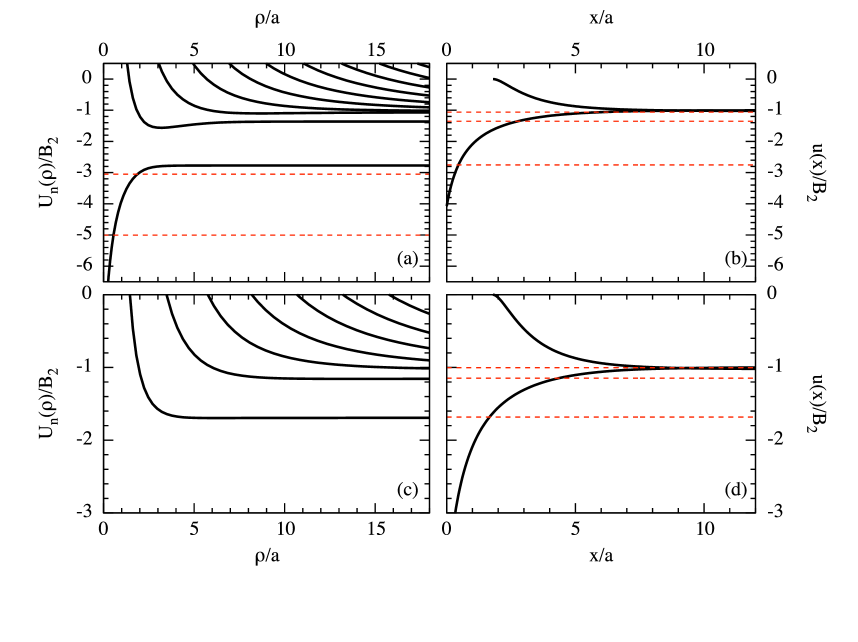
Figure 1: (color online) Graph (a) shows the bosonic hyperradial potential curves describing the heavy-particle dynamics in the HHHL system, while graph (b) shows the corresponding Born-Oppenheimer potential curves for the HHL system. Graphs (c) and (d) show similar curves, except for fermions. All graphs are for $\beta^{-1}=22.08$, appropriate for Li-Cs mixtures. The dashed-red lines indicate bound states.

The atom-dimer scattering length and the HHL spectrum are to a very good approximation determined solely by the potential curve corresponding to the $P=0$ solution to Eq. (14), so we shall restrict our immediate focus to that solution. When the heavy atoms are far apart, $|y-x_{0}|\gg|x_{0}|$, Eq. (5) behaves as though there is a single $\delta$-function of modified strength at the origin. The solutions to Eq. (14) when $x_{0}\rightarrow\infty$ underestimate the correct threshold energy by $\beta/(2+\beta)$:

$$\lim_{|x|\to\infty}{u(x)}=-1-\frac{\beta}{2+\beta}$$ (15)

This result is not unexpected, since we have so far neglected the positive-definite contribution $\tilde{Q}(x)/(2\mu_{3})$ to the heavy-particle kinetic energy. It is known that neglecting this “diagonal correction” — which we call the “Extreme Adiabatic Approximation” (EAA) — yields a lower bound $E_{EAA}$ to the $N$-body bound-state energy. Including the diagonal correction, but neglecting any couplings between Born-Oppenheimer curves — an approximation we call the “uncoupled adiabatic approximation” (UAA) — yields an upper bound $E_{UAA}$ to the correct energy Brattsev (1965); Epstein (1966); Starace and Webster (1979); Coelho and Hornos (1991). We find for this problem that the trend in these inequalities $E_{EAA}<E<E_{UAA}$ is already present in the threshold values of the adiabatic potential itself. In other words, we find that in the limit $|x|\rightarrow\infty$, $u(x)<-1<u(x)+\tilde{Q}(x)/(2\mu_{3})$. In the next section, we explicitly calculate $\tilde{Q}(x)$.

II.2 The Diagonal Correction $\tilde{Q}/(2\mu_{3})$

Using the solutions Eq. (13) (with $A=0$) along with the normalization Eq. (16), we explicitly calculate the integral involved in the nonadiabatic correction Eq. (12). Taking $A=0$ in Eq. (13), continuity of the wavefunction immediately yields $D=B\cosh(\kappa x_{0})/e^{-\kappa x_{0}}$. The remaining normalization constant, $B$, depends on the H-H separation distance both explicitly, and implicitly through the eigenvalue $\kappa$:

$$B(x)=\frac{2\sqrt{\kappa}}{\sqrt{2x_{0}\kappa+e^{2x_{0}\kappa}+1}}$$ (16)

Derivatives of the eigenvalue $\kappa(x)$ are replaced by expressions involving $\kappa$ itself by differentiating Eq. (14) with respect to $x$ and solving for $\kappa^{\prime}$. We find that the nonadiabatic correction $\tilde{Q}(x)$ can be expressed as a rational polynomial in the separation distance $x$:

$$\tilde{Q}(x)=\frac{\beta}{3(2+\beta)\left(-2hx_{0}+2\kappa x_{0}+1\right){}^{4}}$$

$$\times\big{[}3h^{2}+x_{0}\left(-12h^{3}+24h^{2}\kappa-36h\kappa^{2}+24\kappa^{3}\right)+$$

$$x_{0}^{3}\left(-16h^{3}\kappa^{2}+48h^{2}\kappa^{3}-48h\kappa^{4}+16\kappa^{5}\right)+$$

$$x_{0}^{2}\left(12h^{4}-48h^{3}\kappa+108h^{2}\kappa^{2}-120h\kappa^{3}+48\kappa^{4}\right)+$$

$$x_{0}^{4}\left(-16h^{4}\kappa^{2}+64h^{3}\kappa^{3}-96h^{2}\kappa^{4}+64h\kappa^{5}-16\kappa^{6}\right)\big{]},$$ (17)

where we have defined the constant $h=\mu_{3}g_{3}$. Evaluating Eq. (II.2) at the asymptotic value of the potential Eq. (15) gives $\tilde{Q}/2\mu_{3}\rightarrow[\beta/(2+\beta)]+[\beta/(2+\beta)]^{2}$, and including $\tilde{Q}/(2\mu_{3})$ in Eq. (11) yields the correct threshold energy to order $(\frac{\beta}{2+\beta})^{2}$:

$$\lim_{|x|\rightarrow\infty}{\left[u(x)+\frac{\tilde{Q}}{2\mu_{3}}\right]}=-1+\left(\frac{\beta}{2+\beta}\right)^{2}.$$ (18)

In other words, for small $\beta$, the error in the threshold energy vanishes linearly without the diagonal correction, but quadratically when it is included. Interestingly, for the equal mass case ($\beta=1$), the UAA gives the correct threshold energy to within 11%. This may seem a somewhat surprising result since the Born-Oppenheimer factorization is typically expected to fail catastrophically in this limit, however other authors Adhikari et al. (1992) have found the Born-Oppenheimer approach to work surprisingly well for short-range s-wave interactions in 3D for a wide variety of mass ratios. It seems that the present 1D calculation shares similar good-fortune.

II.3 Numerical results for the HHL system

Here, we compare the present Born-Oppenheimer calculation for the HHL system to the high-accuracy calculations of Kartavtsev et al. (2009). Binding energies and scattering solutions are calculated in the UAA.

For the scattering calculation, $u(x)$ and $\tilde{Q}(x)$ are calculated to 15 digits on a uniform grid, and the Numerov method is used to propagate the solution out from $x=0$ to some $x_{max}$. The attractive well in $u(x)$ widens as the mass ratio $\beta^{-1}$ increases. An $x_{max}\sim 40$ is sufficient for $\beta^{-1}\lesssim 10$, but must be increased to $x_{max}\sim 120$ for $\beta^{-1}\sim 250$. For a Numerov step size $s$, each integration step in the Numerov method can introduce an error of order $s^{5}$. For $N_{s}$ total steps, an upper bound to the asymptotic values of the wavefunction of order $N_{s}s^{5}=x_{max}s^{4}$ is maintained less than $10^{-10}$. The asymptotic wavefunction is matched to:

$$\psi(x)\rightarrow\begin{cases}\cos(kx)-\tan(\delta)\sin(kx)\;\;\;\text{Bosons}\\ \sin(kx)+\tan(\delta)\cos(kx)\;\;\;\text{Fermions}\end{cases}$$ (19)

The atom-dimer scattering length is then extracted from the effective range expansion as:

$$\frac{1}{a_{AD}}=\lim_{k_{AD}\rightarrow 0}\begin{cases}k_{AD}\tan{\delta}\;\;\;\text{Bosons}\\ -k_{AD}\cot{\delta}\;\;\;\text{Fermions}\end{cases}$$ (20)

Here, $k_{AD}=\sqrt{2\mu_{23,1}E_{rel}}$, while $k=\sqrt{2\mu_{3}E_{rel}}$. The mass ratios in Table 1 (discussed below) are obtained by a bisection root-finding algorithm (either on $1/a_{AD}$ or on $a_{AD}$) to 6-digit precision. The number of digits reported here represents the precision of our calculation. The accuracy is best estimated by comparing to the calculations of Kartavtsev et al. (2009).

Bound-state calculations are performed variationally by expanding $\psi(x)$ in a basis of b-splines, and solving the resulting generalized eigenvalue problem. We have verified that the results are well converged with respect to the number of grid points used to interpolate the potential $u(x)$, as well as the number and placement of b-splines.

In Fig. 2(a), we show the three-body spectrum as a function of $\beta^{-1/2}$ (recall $\beta=m_{L}/m_{H}$). The mass ratios at which a new state appears, marked by the red crosses for $\lambda=0$ and red dots for $\lambda=\infty$, trace out a curve governed by the $\beta$-dependence of the threshold Eq. (18). In the hyperspherical calculation of Kartavtsev et al. (2009), the threshold is reproduced exactly, and all dots and crosses appear at $E_{2}/B_{2}=-1$.

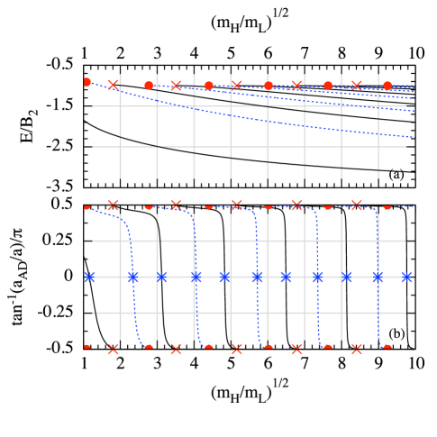
Figure 2: Graph (a) shows the energy spectrum for the three-body (HHL) system as a function $\beta^{-1/2}$. Graph (b) shows $\tan^{-1}{(a_{AD}/a)}/\pi$, where $a_{AD}$ is the atom-dimer scattering length. For both graphs, the solid-black curves denote noninteracting bosonic H-particles. The dashed-blue curves denote noninteracting fermionic particles, or equivalently, fermionized H-particles with $\lambda\rightarrow\infty$. Red crosses and dots, for bosons and fermions respectively, indicate the appearance of a new bound state and $|a_{AD}|\rightarrow\infty$. Blue stars indicate $a_{AD}\rightarrow 0$.

Table 1: The values of the mass ratio $\beta^{-1}=m_{H}/m_{L}$ for which the atom-dimer scattering length is infinite ($a_{AD}\rightarrow\infty$, corresponding to the appearance of the $n^{\text{th}}$ trimer state), or zero ($a_{AD}\rightarrow 0$), are tabulated both the case of noninteracting bosonic H atoms ($\lambda\rightarrow 0$) and fermionic H atoms ($\lambda\rightarrow\infty$). Results are compared to Ref. Kartavtsev et al. (2009). An asterisk (*) denotes an exact result.

	$\lambda=0$		$\lambda=0$
$n$	$\beta^{-1}\large|_{a_{AD}\rightarrow 0}$		$\beta^{-1}\large|_{a_{AD}\rightarrow\infty}$
	This work	Ref. Kartavtsev et al. (2009)	This work	Ref. Kartavtsev et al. (2009)
1	$-$	$-$	$-$	$-$
2	$1.357$	$0.971$	$3.255$	$2.86954$
3	$9.747$	$9.365$	$12.336$	$11.9510$
4	$23.333$	$22.951$	$26.602$	$26.218$
5	$42.142$	$41.762$	$46.055$	$45.673$
6	$66.168$	$65.791$	$70.695$	$70.317$
7	$95.404$	$95.032$	$100.523$	$100.151$
8	$129.845$	$129.477$	$135.539$	$135.170$
9	$169.488$	$169.120$	$175.742$	$175.374$
10	$214.331$	$213.964$	$221.133$	$220.765$

	$\lambda=\infty$		$\lambda=\infty$
$n$	$\beta^{-1}\large|_{a_{AD}\rightarrow 0}$		$\beta^{-1}\large|_{a_{AD}\rightarrow\infty}$
	This work	Ref. Kartavtsev et al. (2009)	This work	Ref. Kartavtsev et al. (2009)
1	$-$	$0^{*}$	$1.170$	$1^{*}$
2	$5.499$	$5.2107$	$7.694$	$7.3791$
3	$16.456$	$16.1197$	$19.373$	$19.0289$
4	$32.650$	$32.298$	$36.235$	$35.879$
5	$54.067$	$53.709$	$58.283$	$57.923$
6	$80.697$	$80.339$	$85.518$	$85.159$
7	$112.535$	$112.179$	$117.940$	$117.583$
8	$149.577$	$149.222$	$155.550$	$155.193$
9	$191.820$	$191.463$	$198.347$	$197.989$
10	$239.262$	$238.904$	$246.331$	$245.973$

Figure 2(b) shows $\tan^{-1}{(a_{AD}/a)}/\pi$ as a function of $\beta^{-1/2}$. Again, the red dots and crosses denote the mass ratios at which a new state appears and the atom-dimer scattering length $a_{AD}\rightarrow\infty$. The blue stars indicate $a_{AD}\rightarrow 0$. In a manner similar to Kartavtsev et al. (2009), we tabulate these particular values of the mass ratio in Table 1. Note that the Born-Oppenheimer calculation consistently overestimates the critical mass ratios $\beta^{-1}$ by approximately $0.3-0.4$. The overestimate is understood, at least qualitatively, by noting that the $UAA$ produces an upper bound to the binding energy, and the trend in the spectrum is for deeper binding as $\beta^{-1}$ increases. The percentage error in the critical values of $\beta^{-1}$ decreases monotonically, as one might expect.

The $\beta=1$ HHL ground state for $\lambda=0$ bosons was found in Kartavtsev et al. (2009) to be (in units of $B_{2}$) $E_{3}=-2.087719$, very close to the value $E_{3}=-2.08754$ found much earlier in Gaudin and Derrida (1975). Here, we find that the EAA produces a lower bound of $E_{3,EAA}=-2.4227$, approximately 16% deeper than the correct value. The UAA underbinds by about 11%, giving the upper bound $E_{3,UAA}=-1.8561$. It is interesting that the error in the UAA calculation is almost entirely accounted for by the overestimate of the atom-dimer threshold energy. In fact, scaling by the threshold energy Eq. (18), one obtains $E_{3,UAA}/E_{\text{thresh}}=-2.0879$, overbinding by only $0.01\%$.

Kartavtsev and Malykh Kartavstev and Malykh (2007) found that universal (non-Efimov) fermionic states in 3D exist for mass ratios $\beta^{-1}\gtrsim 8.17$. Pricoupenko and Pedri Pricoupenko and Pedri (2010) found similar states in 2D for $\beta^{-1}\gtrsim 3.33$. Levinsen and Parish Levinsen and Parish (2013) established that these states are continuously connected as confinement is increased. It is interesting to speculate whether the fermionic state that appears in 1D at $\beta^{-1}=1$ ($\beta^{-1}\approx 1.170$ in our calculation) is continuously connected to these universal trimer states in higher dimensions.

III Four-Body (HHHL) Problem

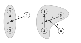
Figure 3: A schematic diagram of the Jacobi coordinates for (a) the three-body problem and (b) the four-body problem are shown. The heavy particles are contained in the shaded regions.

Let us now turn to the calculation of four-body observables. The basic three-step recipe for this calculation is as follows. First, the Born-Oppenheimer method is used to calculate the 2D potential energy surface for the heavy particles in the extreme adiabatic approximation (EAA). Next, this potential energy surface is inserted into a calculation of the hyperradial adiabatic potential curves and couplings. Finally, the resulting set of coupled hyperradial equations is solved for the bound-states and atom-trimer scattering length. The entire procedure is then repeated for different values of $\beta$. If a sufficiently large number of hyperradial curves and couplings are included in the final step, then the accuracy of the calculation is limited almost entirely by the EAA made in the first step.

III.1 The adiabatic equations

For all four-body (HHHL) calculations that follow, we choose particles 1, 2 and 3 to have mass $m_{1}=m_{2}=m_{3}=m_{H}$ and particle 4 to have mass $m_{4}=\beta m_{H}$. The solution to the adiabatic equation is most easily carried out using the “K-type” Jacobi coordinates shown in Fig. 3(b), with unitless mass-scaled coordinates defined as:

$$x =\frac{1}{a}\sqrt{\frac{\mu_{12}}{\mu_{4b}}}\left(x_{1}-x_{2}\right)$$

$$y =\frac{1}{a}\sqrt{\frac{\mu_{12,3}}{\mu_{4b}}}\left(\frac{m_{1}x_{1}+m_{2}x_{2}}{m_{1}+m_{2}}-x_{3}\right)$$

$$z =\frac{1}{a}\sqrt{\frac{\mu_{123,4}}{\mu_{4b}}}\left(\frac{m_{1}x_{1}+m_{2}x_{2}+m_{3}x_{3}}{m_{1}+m_{2}+m_{3}}-x_{4}\right)$$ (21)

Here, $\mu_{4b}=(\mu_{12}\mu_{12,3}\mu_{123,4})^{1/3}$ is the four-body reduced mass. Again, we rescale the Schrödinger equation by the heavy-light binding energy $B_{2}$. The full four-body Schrödinger equation then reads:

$$\begin{split}\frac{-1}{2\mu_{4}}&\nabla^{2}\Psi(\rho,\phi,z)+\Big{[}g_{4}\sum_{i=1}^{3}{\delta(z-z_{i})}\\ +&\lambda g_{4}\sum_{i<j}^{3}{\delta\left(\alpha\rho\left|\sin(\phi-\phi_{ij})\right|\right)}\Big{]}\Psi(\rho,\phi,z)=E\Psi(\rho,\phi,z)\end{split}$$ (22)

where $\alpha=\sqrt{6}[(3+\beta)/\beta]^{1/6}$, $\phi_{12}=\pi/2$, and $\phi_{23}=-\phi_{13}=\pi/6$. Again, rescaling by $B_{2}$ introduces the following unitless parameters:

$$\mu_{4} =\frac{\beta+1}{2\beta^{2/3}(3+\beta)^{1/3}}$$ (23)

$$g_{4} =-2\sqrt{3}\left({\frac{\beta}{3+\beta}}\right)^{1/3}$$ (24)

$$z_{i} =\sqrt{\frac{2\beta}{3+\beta}}\;\rho\sin\left(\phi-\phi_{i}\right)$$ (25)

where $\phi_{1}=-4\pi/3$, $\phi_{2}=0$, and $\phi_{3}=-2\pi/3$. The particular choice of Jacobi coordinates Eq. (III.1) has the advantage that the separation distances $x_{12}$, $x_{13}$ and $x_{23}$ are all independent of the $z$-coordinate. The heavy-particle dynamics is restricted to the $x$-$y$ plane, and the light particle can be integrated out by solving an equation in the $z$-coordinate only, with fixed $x$ and $y$. The transformation to hyperspherical coordinates is accomplished by expressing $x$, $y$, and $z$ in terms of the usual spherical polar coordinates $R$, $\theta$ and $\phi$. The heavy-particle subsector is then described by $x=\rho\cos\phi$ and $y=\rho\sin\phi$, where $\rho=\sqrt{x^{2}+y^{2}}$ is the projection of $R$ onto the $x$-$y$ plane: $\rho=R\sin\theta$, and $z=R\cos\theta$.

Clearly, fixing $x$ and $y$ is equivalent to fixing $\rho$ and $\phi$. We make the Born-Oppenheimer factorization:

$$\Psi=\Phi(\rho,\phi;z)\psi(\rho,\phi),$$ (26)

where the adiabatic equation for the Born-Oppenheimer surface is:

$$\begin{split}\left(\frac{-1}{2\mu_{4}}\frac{\partial^{2}}{\partial z^{2}}+g_{4}\sum_{i=1}^{3}{\delta(z-z_{i})}\right)\Phi(\rho,\phi;z)=U(\rho,\phi)\Phi(\rho,\phi;z)\end{split}$$ (27)

The heavy-particle eigenstates now live on the potential energy surface $U(\rho,\phi)$, and satisfy (in the EAA):

$$\begin{split}&\frac{-1}{2\mu_{4}}\left(\frac{1}{\rho}\frac{\partial}{\partial\rho}\rho\frac{\partial}{\partial\rho}+\frac{1}{\rho^{2}}\frac{\partial^{2}}{\partial\phi^{2}}\right)\psi(\rho,\phi)\\ &+\left[U(\rho,\phi)+\lambda g_{4}\sum_{i<j}^{3}{\delta\left(\alpha\rho\left|\sin(\phi-\phi_{ij})\right|\right)}\right]\psi(\rho,\phi)\\ &=E_{EAA}\psi(\rho,\phi)\end{split}$$ (28)

Finally, we describe $\psi(\rho,\phi)$ as a sum over adiabatic channel functions:

$$\psi(\rho,\phi)=\sum_{n=0}^{\infty}{\rho^{-1/2}f_{n}(\rho)\chi_{n}(\rho;\phi)},$$ (29)

where $\chi_{n}(\rho;\phi)$ satisfy the fixed-$\rho$ equation:

$$\begin{split}&\frac{-1}{2\mu_{4}\rho^{2}}\frac{\partial^{2}\chi_{n}}{\partial\phi^{2}}+U(\rho,\phi)\chi_{n}\\ &+\lambda g_{4}\sum_{i<j}^{3}{\delta\left(\alpha\rho\left|\sin(\phi-\phi_{ij})\right|\right)}\chi_{n}=U_{n}(\rho)\chi_{n}\end{split}$$ (30)

Because we only consider $\lambda=0$ and $\lambda\rightarrow\infty$, the $\delta$-functions in Eq. (30) result in simple boundary conditions at $\phi=\pi/6$. For arbitrary $\lambda$, one would need to account for the $\lambda$-dependent derivative discontinuity at $\phi=\pi/6$. Inserting the expansion Eq. (29) into Eq. (28) results in a set of coupled equations in $\rho$, which are conveniently written in matrix form as:

$$\begin{split}\frac{-1}{2\mu_{4}}&\left(\mathbf{1}\frac{\partial^{2}}{\partial\rho^{2}}+\mathbf{Q}(\rho)+2\mathbf{P}(\rho)\frac{\partial}{\partial\rho}\right)\vec{f}(\rho)\\ &+\mathbf{U}_{\text{eff}}(\rho)\vec{f}(\rho)=E_{EAA}\vec{f}(\rho)\end{split}$$ (31)

Here, $\mathbf{U}_{\text{eff}}$ is a diagonal matrix with elements $U_{n}(\rho)-1/8\mu_{4}\rho^{2}$, $P_{mn}(\rho)=\left\langle\chi_{m}\left|\frac{\partial\chi_{n}}{\partial\rho}\right.\right\rangle_{\phi}$ and $Q_{mn}(\rho)=\left\langle\chi_{m}\left|\frac{\partial^{2}\chi_{n}}{\partial\rho^{2}}\right.\right\rangle_{\phi}$. When $\mathbf{P}$ and $\mathbf{Q}$ are included in the solution to Eq. (31), and enough channels are retained for numerical convergence, the accuracy of the four-body energy is (in principle) limited only by the omission of first and second derivative couplings, $\left\langle\Phi_{m}\left|\vec{\nabla}\Phi_{n}\right.\right\rangle_{z}$ and $\left\langle\Phi_{m}\left|\nabla^{2}\Phi_{n}\right.\right\rangle_{z}$, that arise from generalizing Eq. (26) to include a sum: $\Psi=\sum_{n}{\Phi_{n}\psi_{n}}$. Such a generalization is not possible for our model without the introduction of a confining potential because Eq. (27) admits only one solution that vanishes as $|z|\rightarrow\infty$.

Identical particle symmetry of the heavy particles allows one to restrict the domain of the four-body wavefunction to the region $0<\phi<\pi/6$. Thus, for a given permutation of heavy particles, the locus of points describing the coalescence of a heavy particle and a light particle — i.e. when $z$ is equal to $z_{i}$ — remain ordered $z_{1}<z_{2}<z_{3}$ along the $z$-coordinate. Because the ordering is independent of $\rho$ and $\phi$, the solution to Eq. (27) for all $\rho$ and all $\phi\in[0,\pi/6]$ is straightforward.

The boundary condition on $\chi(\rho;\phi)$ at $\phi=0$ is determined by a combination of the parity operator, $\hat{\Pi}\phi\rightarrow\phi+\pi$, and the 1-2 permutation operator, $\hat{P}_{12}\phi\rightarrow\pi-\phi$, by the rule: $\hat{P}_{12}\hat{\Pi}\phi\rightarrow-\phi$. Considering positive parity, the boundary conditions on $\chi(\rho;\phi)$ for noninteracting bosons are: $\left.\frac{\partial\chi}{\partial\phi}\right|_{\phi=0}=\left.\frac{\partial\chi}{\partial\phi}\right|_{\phi=\pi/6}=0$, while for noninteracting fermions, $\chi|_{\phi=0}=\chi|_{\phi=\pi/6}=0$. Note that the boundary conditions for noninteracting fermions of positive parity are equivalent to those for bosons of negative parity, but $\lambda\rightarrow\infty$.

III.2 Numerical Solutions for the HHHL System

In Appendix A, we calculate the transcendental equation for the eigenvalue of a 1D Schrödinger equation with three $\delta$-functions of arbitrary strength and arbitrary placement. The resulting Eq. (A) is applied to the Eq. (27) by letting $g_{a}=g_{b}=g_{c}=2\mu_{4}g_{4}$, $\kappa^{2}=-2\mu_{4}U(\rho,\phi)>0$, and $a=z_{1}$, $b=z_{2}$ and $c=z_{3}$.

Figure. 4 shows the potential energy surface for the particular mass ratio $\beta^{-1}=22.08$ appropriate for an atomic mixture of Li-Cs. Potential surfaces like this one are calculated by solving Eq. (A) on a nonlinear grid with typically $200\times 400$ points in the $(\rho,\phi)$ plane. The points are distributed so that more grid-points are concentrated in the vicinity of the well at $\rho=0$ and the valley near $\phi=\pi/6$. Particular care must be taken to describe the valley near $\phi=\pi/6$ accurately at large $\rho$, or else the numerical solution to the fixed-$\rho$ adiabatic equation does not reproduce the correct threshold behavior in any of the atom-trimer channels. This is because the fixed-$\rho$ solutions as $\rho\rightarrow\infty$ should approach the HHL bound-state energies from the spectrum in Fig. 2 with the correct $\rho$-dependence. In particular, at large $\rho$ we find that $Q_{00}(\rho)/2\mu_{4}\rightarrow-1/8\mu_{4}\rho^{2}$, and exactly cancels the $+1/8\mu_{4}\rho^{2}$ in the $U_{0,\text{eff}}$. That is, the effective potential with the diagonal correction approaches a constant, and describes a 2-body channel to which Eqs. (19) and (20) may be applied with the replacements $\psi\rightarrow f$, $k_{AD}\rightarrow k_{AT}=\sqrt{2\mu_{234,1}E_{\text{rel}}}$, $a_{AD}\rightarrow a_{AT}$, and $x\rightarrow\rho$, along with the boundary condition $f(0)=0$.

Figures 1(a) and 1(c) show the hyperradial potential curves $U_{n}(\rho)$ obtained by solving the fixed-$\rho$ Eq. (30) using the potential energy surface shown in Fig. 4. Note that at large $\rho$, the lowest potential curves converge to the appropriate HHL bound state energy shown as red dashed lines in Fig. 1(b) and 1(d), as appropriate for an atom-trimer channel. The red dashed lines in Fig. 1(a) and (c) indicate HHHL bound states obtained by solving Eq. (31) with 10 coupled channels. Typically, calculations with only the lowest channel (but including the diagonal correction) give bound-state energies converged to four or five digits. The error incurred by ignoring excited hyperradial potential curves is expected to be negligible compared to making the EAA in the calculation of the surface $U(\rho,\phi)$.

In Figures 5 and 6, we show the spectrum and atom-trimer scattering lengths of the HHHL system with noninteracting bosonic and fermionic heavy atoms, respectively. We show both positive (B+, F+), and negative (B-, F-) parity cases for each identical particle symmetry. The HHL ground-state energies for each symmetry from Fig. 2(a) are replotted here as dashed-red curves. Again, mass ratios at which a new tetramer state appears (and $|a_{AT}|\rightarrow\infty$) are marked by red crosses, while zeroes of $a_{AT}$ are indicated by blue stars. The particular numerical values for the coordinates $(\beta^{-1/2},E/B_{2})$ are also marked. As the mass-ratio $\beta^{-1}$ increases, four-body bound states enter at lower energies than one would expect from the three-body calculation (i.e. the dashed-red curve). This discrepancy in the threshold energy is attributed to the fact that the EAA underestimates the potential surface in Fig. 4 by neglecting the positive nonadiabatic correction $-\left\langle\Phi\right|\left.\nabla^{2}\Phi\right\rangle_{z}/2\mu_{4}$, while the corresponding correction is included at the three-body level in Fig. 2.

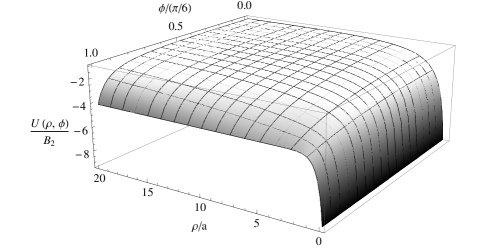
Figure 4: The Born-Oppenheimer surface for the HHHL system is shown. $U(\rho,\phi$) is in units of $B_{2}$, and $\rho$ is in units of $a$.

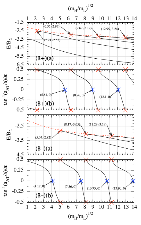
Figure 5: Graphs (B+)(a) and (B-)(a) show the HHHL spectrum for bosonic heavy particles of positive and negative parity, respectively. The red crosses indicate the appearance of a new HHHL bound state and $a_{AT}\rightarrow\infty$. The red dashed curve is the lowest (solid line) bosonic HHL bound state from Fig. 2(a). Graphs (B+)(b) and (B-)(b) show the arctangent of the atom-trimer scattering length for bosonic heavy particles of positive and negative parity, respectively. The blue stars indicate $a_{AT}\rightarrow 0$. The specific ordinates of the crosses and stars are labeled.

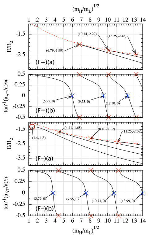
Figure 6: Graphs (F+)(a) and (F-)(a) show the HHHL spectrum for fermionic heavy particles of positive and negative parity, respectively. The red crosses indicate the appearance of a new HHHL bound state and $a_{AT}\rightarrow\infty$. The red dashed curve is the lowest (solid line) fermionic HHL bound state from Fig. 2(a). Graphs (F+)(b) and (F-)(b) show the arctangent of the atom-trimer scattering length for fermionic heavy particles of positive and negative parity, respectively. The blue stars indicate $a_{AT}\rightarrow 0$. The specific ordinates of the crosses and stars are labeled.

While we perform a multichannel calculation of the spectrum, we find that it is sufficient to use a simple single-channel calculation for $a_{AT}$. Indeed, comparing the critical mass ratios for which $a_{AT}\rightarrow\infty$, and a tetramer state lies at threshold, we find good agreement between the two calculations. This can be readily observed by comparing the positions of the red crosses in graphs (a) and (b) of Fig. 5, and similarly in Fig. 6.

At $\beta=1$, we find that noninteracting bosons of positive parity admit an HHHL bound state with $E_{4,\text{EAA}}\approx-3.55$. The second tetramer state appears at $\beta^{-1}\approx 4.88$, and the third at $\beta^{-1}\approx 40.3$. For Li-Cs mixtures, one might expect two universal tetramer states. Negative parity bosons are less likely to bind than those with positive parity. The first tetramer state appears at $\beta^{-1}\approx 25.4$, and the second at $\beta^{-1}\approx 66.7$.

For fermionic particles, negative parity tetramers are more likely to bind than those with positive parity. The precise value of the critical mass ratio is difficult to pin down within the Born-Oppenheimer approximation at these small mass ratios. The difficulty is magnified because even in the UAA three-body calculations of Section II, the trimer state doesn’t appear until $\beta^{-1}\approx 1.17$. Because the four-body calculation doesn’t include the positive nonadiabatic correction to the potential energy surface shown in Fig. 4, One expects the tetramer bound state to appear below the atom-trimer threshold prematurely. In the four-body calculation, the energy of the atom trimer threshold itself increases slightly with $\beta^{-1/2}$, and the tetramer energy tracks along with it until about $\beta^{-1}\approx 2.6$. The increasing threshold energy is undoubtedly an artifact of the approximation at the four-body level since it is absent in the more accurate three-body calculations. We can nonetheless estimate the critical mass ratio as $\beta^{-1}\approx 2.0\pm 0.6$, indicated by a red circle in Fig. 6(F-)(a). The second negative parity fermionic state appears at $\beta^{-1}=19.4$.

In 3D, Blume Blume (2012) found that a universal tetramer exists for fermionic particles above a mass ratio of $\beta^{-1}\approx 9.5$. In 2D, Levinsen and Parish Levinsen and Parish (2013) found a critical mass ratio of $\beta^{-1}\approx 5.0$. It is interesting to speculate whether these states are continuously connected to each other, and to the universal state that appears in these calculations at $\beta^{-1}\approx 2.0$ for negative parity fermions.

IV Summary and Outlook

We have calculated three-body and four-body spectra, as well as the atom-dimer and atom-trimer scattering lengths for two-component systems with one light particle, as a function of the mass ratio. Heavy particles are assumed to be noninteracting, and the four-particle system is assumed to be in free-space. Both bosonic and fermionic heavy particles are treated. For the HHL system, the Born-Oppenheimer method gives good quantitative agreement with the hyperspherical calculations of Kartavtsev et al. (2009). For the HHHL system, the potential energy surface governing the heavy-particle dynamics is calculated in the “extreme adiabatic approximation”. That surface is then used to calculate hyperradial potential curves and couplings. The values for the resulting atom-trimer thresholds converge to the appropriate three-body bound state energies, lending some confidence to the HHHL calculation.

Let us now discuss possible extensions of this work. Note that we have scaled away the only length scale, $a$, that appears in our model. There are two immediate generalizations that expand the parameter space considerably.

First, there is the generalization to arbitrary H-H interactions, which introduces the H-H scattering length $a_{HH}$. Such an extension was already treated at the three-body level in Kartavtsev et al. (2009), but no such four-body calculations have appeared in the literature. In a hyperspherical calculation, the additional derivative discontinuity in the angular wavefunction is treated analytically, and the hyperradial potential curves are calculated as the solution to a single transcendental equation Mehta et al. (2007); Kartavtsev et al. (2009). The HHHL Born-Oppenheimer calculation for bosons can be extended to arbitrary $\lambda$ by choosing a b-spline basis set that satisfies the boundary condition,

$$\lim_{\epsilon\rightarrow 0}{\left.\frac{1}{\chi}\frac{\partial\chi}{\partial\phi}\right|_{\pi/6-\epsilon}}=\frac{\rho\lambda(1+\beta)}{\sqrt{2}\beta}\left(\frac{\beta}{3+\beta}\right)^{5/6}$$ (32)

With this generalization, one can smoothly transition between the energies shown in Fig. 5 and Fig. 6, passing from noninteracting bosons to the fermionized limit.

The bound-state calculation can be extended by the introduction of a harmonic trapping potential, which separates into relative and center-of-mass parts under the transformation to Jacobi coordinates. This extension would establish a connection with several papers that have appeared recently, treating equal-mass two-component systems Gharashi and Blume (2013); Sowiński et al. (2013); Lindgren et al. (2013). The addition of a trapping potential would introduce excited potential energy surfaces and the possibility of interesting physics beyond the Born-Oppenheimer approximation.

Here, we have only considered the “3+1” branch (i.e. the HHHL system) of the few-component problem. It may be that other branches can be treated by similar methods. For example, for the 2+2 (HHLL) problem, integrating out the light atoms would result in a 1D heavy-heavy potential, but the adiabatic equation is a 2D partial differential equation, instead of a 1D equation like Eq. (27).

Finally, it is worth emphasizing that ultimately a fully 3D solution to the few-body problem with finite-range interactions is needed in order to understand the physics of quasi-1D systems. A hyperspherical solution to the few-body problem in quasi-1D for finite-range interactions remains a significant challenge, although recent advances in the Correlated Gaussian Hyperspherical method Daily and Greene (2014) may make these calculations possible.

Appendix A Triple $\delta$-function problem

Here, we give the solution for the eigenvalue to the following Schrödinger equation:

$$\begin{split}&\left[-\frac{\partial^{2}}{\partial z^{2}}+g_{a}\delta(z-a)+g_{b}\delta(z-b)+g_{c}\delta(z-c)\right]\Phi(z)\\ &=-\kappa^{2}\Phi(z)\end{split}$$ (33)

We assume that the positions of the $\delta$-functions are ordered as $a<b<c$, but no other assumptions regarding their placement are made. In particular, the Hamiltonian is not assumed to commute with the parity operator. The (unnormalized) solution satisfying asymptotic boundary condition, $\Phi(|z|\rightarrow\infty)=0$, is elementary:

$$\Phi(z)=\begin{cases}\Phi_{I}&=Ae^{\kappa z}\;\;z<a\\ \Phi_{\text{II}}&=Be^{-\kappa z}+Ce^{\kappa z}\;\;a<z<b\\ \Phi_{\text{III}}&=De^{-\kappa z}+Ee^{\kappa z}\;\;b<z<c\\ \Phi_{\text{IV}}&=Fe^{-\kappa z}\;\;c<z\end{cases}$$ (34)

Matching the solutions and enforcing the derivative discontinuities at $z=a$, $z=b$, and $z=c$ yields, after considerable algebra:

$$g_{a}g_{c}(g_{b}-2\kappa)e^{2\kappa(a+b)}-g_{a}g_{b}(g_{c}+2\kappa)e^{2\kappa(a+c)}$$

$$+(g_{a}+2\kappa)(g_{b}+2\kappa)(g_{c}+2\kappa)e^{2\kappa(b+c)}$$

$$-g_{b}g_{c}e^{4b\kappa}(g_{a}+2\kappa)=0$$ (35)

For the special case of a quadrupolar potential ($a=-c$, $b=0$ and $g_{a}=g_{c}=-g_{b}/2$), Eq. A reduces to the result found recently by Patil Patil (2009).

References

- Greiner et al. (2001) M. Greiner, I. Bloch, O. Mandel, T. W. Hänsch, and T. Esslinger, Phys. Rev. Lett. 87, 160405 (2001).
- Görlitz et al. (2001) A. Görlitz, J. M. Vogels, A. E. Leanhardt, C. Raman, T. L. Gustavson, J. R. Abo-Shaeer, A. P. Chikkatur, S. Gupta, S. Inouye, T. Rosenband, and W. Ketterle, Phys. Rev. Lett. 87, 130402 (2001).
- B. Laburthe Tolra and K. M. O’Hara and J. H. Huckans and W. D. Phillips and S. L. Rolston and J. V. Porto (2004) B. Laburthe Tolra and K. M. O’Hara and J. H. Huckans and W. D. Phillips and S. L. Rolston and J. V. Porto, Phys. Rev. Lett. 92, 190401 (2004).
- Kinoshita et al. (2004) T. Kinoshita, T. Wenger, and D. S. Weiss, Science 305, 1125 (2004).
- Kinoshita et al. (2006) T. Kinoshita, T. Wenger, and D. S. Weiss, Nature 440, 900 (2006).
- Leanhardt et al. (2002) A. E. Leanhardt, A. P. Chikkatur, D. Kielpinski, Y. Shin, T. L. Gustavson, W. Ketterle, and D. E. Pritchard, Phys. Rev. Lett. 89, 040401 (2002).
- Fried et al. (1998) D. G. Fried, T. C. Killian, L. Willmann, D. Landhuis, S. C. Moss, D. Kleppner, and T. J. Greytak, Phys. Rev. Lett. 81, 3811 (1998).
- Parker et al. (2012) R. H. Parker, M. R. Dietrich, K. Bailey, J. P. Greene, R. J. Holt, M. R. Kalita, W. Korsch, Z.-T. Lu, P. Mueller, T. P. O’Connor, J. Singh, I. A. Sulai, and W. L. Trimble, Phys. Rev. C 86, 065503 (2012).
- Ni et al. (2008) K.-K. Ni, S. Ospelkaus, M. De Miranda, A. Pe’er, B. Neyenhuis, J. Zirbel, S. Kotochigova, P. Julienne, D. Jin, and J. Ye, Science 322, 231 (2008).
- Barontini et al. (2009) G. Barontini, C. Weber, F. Rabatti, J. Catani, G. Thalhammer, M. Inguscio, and F. Minardi, Phys. Rev. Lett. 103, 043201 (2009).
- Hara et al. (2011) H. Hara, Y. Takasu, Y. Yamaoka, J. M. Doyle, and Y. Takahashi, Phys. Rev. Lett. 106, 205304 (2011).
- Lieb and Liniger (1963) E. Lieb and W. Liniger, Phys. Rev. 130, 1605 (1963).
- J. B. McGuire (1964) J. B. McGuire, J. Math. Phys. 5, 622 (1964).
- Yang (1967) C. N. Yang, Phys. Rev. Lett. 19, 1312 (1967).
- Yang and Yang (1969) C. Yang and C. Yang, J. Math. Phys. 10, 1115 (1969).
- Dodd (1970) L. Dodd, J. Math. Phys. 11, 207 (1970).
- H. B. Thacker (1974) H. B. Thacker, Phys. Rev. D 11, 838 (1974).
- Gibson et al. (1987) W. G. Gibson, S. Y. Larsen, and J. Popiel, Phys. Rev. A 35, 4919 (1987).
- A. Amaya-Tapia and S.Y. Larsen and J. Popiel (1997) A. Amaya-Tapia and S.Y. Larsen and J. Popiel, Few-Body Syst. 23, 87 (1997).
- Mehta and Shepard (2005) N. P. Mehta and J. R. Shepard, Phys. Rev. A 72, 032728 (2005).
- Mehta et al. (2007) N. P. Mehta, B. D. Esry, and C. H. Greene, Phys. Rev. A 76, 022711 (2007).
- Chuluunbaatar et al. (2006) O. Chuluunbaatar, A. Gusev, M. Kaschiev, V. Kaschieva, A. Amaya-Tapia, S. Larsen, and S. Vinitsky, J. Phys. B: At. Mol. Opt. Phys. 39, 243 (2006).
- Kartavtsev et al. (2009) O. I. Kartavtsev, A. V. Malykh, and S. A. Sofianos, ZhETF 135, 419 (2009).
- Orso et al. (2010) G. Orso, E. Burovski, and T. Jolicoeur, Phys. Rev. Lett. 104, 065301 (2010).
- Macek (1968) J. H. Macek, J. Phys. B: At. Mol. Opt. Phys. 1, 831 (1968).
- Castin et al. (2010) Y. Castin, C. Mora, and L. Pricoupenko, Phys. Rev. Lett. 105, 223201 (2010).
- Guevara et al. (2012) N. L. Guevara, Y. Wang, and B. D. Esry, Phys. Rev. Lett. 108, 213202 (2012).
- Petrov et al. (2007) D. S. Petrov, G. E. Astrakharchik, D. J. Papoular, C. Salomon, and G. V. Shlyapnikov, Phys. Rev. Lett. 99, 130407 (2007).
- Olshanii (1998) M. Olshanii, Phys. Rev. Lett. 81, 938 (1998).
- Bergeman et al. (2003) T. Bergeman, M. G. Moore, and M. Olshanii, Phys. Rev. Lett. 91, 163201 (2003).
- Mora et al. (2005a) C. Mora, R. Egger, and A. O. Gogolin, Phys. Rev. A 71, 052705 (2005a).
- Mora et al. (2005b) C. Mora, A. Komnik, R. Egger, and A. O. Gogolin, Phys. Rev. Lett. 95, 080403 (2005b).
- Levinsen et al. (2014) J. Levinsen, P. Massignan, and M. Parish, (2014), arXiv:1402.1859 [cond-mat.quant-gas] .
- Girardeau (1960) M. D. Girardeau, J. Math Phys. 1, 516 (1960).
- Brattsev (1965) V. F. Brattsev, Sov. Phys. Dokl. 10 (1965).
- Epstein (1966) S. T. Epstein, J. Chem. Phys. 44, 836 (1966).
- Starace and Webster (1979) A. F. Starace and G. L. Webster, Phys. Rev. A 19, 1629 (1979).
- Coelho and Hornos (1991) H. T. Coelho and J. E. Hornos, Phys. Rev. A 43, 6379 (1991).
- Adhikari et al. (1992) S. K. Adhikari, V. Brito, H. Coelho, and T. Das, Il Nuovo Cimento B Series 11 107, 77 (1992).
- Gaudin and Derrida (1975) M. Gaudin and B. Derrida, J. de Phys. 36, 1183 (1975).
- Kartavstev and Malykh (2007) O. Kartavstev and A. Malykh, J. Phys. B: At. Mol. Opt. Phys. 40, 1429 (2007).
- Pricoupenko and Pedri (2010) L. Pricoupenko and P. Pedri, Phys. Rev. A 82, 033625 (2010).
- Levinsen and Parish (2013) J. Levinsen and M. M. Parish, Phys. Rev. Lett. 110, 055304 (2013).
- Blume (2012) D. Blume, Phys. Rev. Lett. 109, 230404 (2012).
- Gharashi and Blume (2013) S. E. Gharashi and D. Blume, Phys. Rev. Lett. 111, 045302 (2013).
- Sowiński et al. (2013) T. Sowiński, T. Grass, O. Dutta, and M. Lewenstein, Phys. Rev. A 88, 033607 (2013).
- Lindgren et al. (2013) E. J. Lindgren, J. Rotureau, C. Forssén, A. G. Volosniev, and N. T. Zinner, (2013), arXiv:1304.2992v1 [cond-mat] .
- Daily and Greene (2014) K. M. Daily and C. H. Greene, Phys. Rev. A 89, 012503 (2014).
- Patil (2009) S. Patil, Eur. J. Phys. 30, 629 (2009).