Chirality asymptotic behavior and non-Markovianity in quantum walks on a line

Abstract

We investigate the time evolution of the chirality reduced density matrix for a discrete-time quantum walk on a one-dimensional lattice, which is obtained by tracing out the spatial degree of freedom. We analyze the standard case, without decoherence, and the situation where decoherence appears in the form of broken links in the lattice. By examining the trace distance for possible pairs of initial states as a function of time, we conclude that the evolution of the reduced density matrix is non-Markovian, in the sense defined in [H. P. Breuer, E. M. Laine, and J. Piilo, Phys. Rev. Lett. 103, 210401 (2009)]. As the level of noise increases, the dynamics approaches a Markovian process. The highest non-Markovianity corresponds to the case without decoherence. The reduced density matrix tends always to a well-defined limit that we calculate, but only in the decoherence-free case this limit is non-trivial.

I Introduction

Markov approximation is a valuable and powerful tool for studying the dynamics of an open system interacting with its environment. It holds when full predictions on the future evolution of the system can be obtained by only knowing its present state, and no further knowledge of its past is required. The classical random walk is an example of Markovian process that has found applications in many fields. In quantum mechanics, important physical processes leading to decoherence can be analyzed by means of simple Markovian models. For instance, in quantum optics, the time evolution of an open system characterized by a non-unitary behavior can be described by a master equation written generally in the form of a Lindblad equation BreuerPetruccione .

In quantum information theory, the discrete-time quantum walk (QW) on a line has been studied as a natural generalization of the classical random walk Aharonov . In this context, it has been shown in detail how the unitary quantum mechanical evolution of the QW can be separated into Markovian and interference terms alejo2003 ; alejo2004 . The Markovian terms responsible for the diffusion obey a master equation, while the others include the interference terms needed to preserve the unitary character of the evolution. This approach provides an intuitive framework which becomes useful for analyzing the behavior of quantum systems in which decoherence plays a central role. In other words, this formalism shows in a transparent form that the primary effect of decoherence here is to make the interference terms negligible in the evolution equation, and then the Markovian behavior is immediately obtained.

In this scenario, it is important to find a way to evaluate how non-Markovian a quantum system is. Ref. Breuer2009 has proposed a general measure for the degree of non-Markovian behavior in open quantum systems. This measure is based on the trace distance, which quantifies the distinguishability of quantum states, and can be interpreted in terms of the information flow between the open system and its environment. The measure takes nonzero values whenever there is a flow of information from the environment back to the open system, and it has already been used in different contexts BreuerUses .

On the other hand, the asymptotic behavior of the QW has been recently investigated focusing on the chirality reduced density matrix, obtained when the position degree of freedom is traced out alejo2010 ; alejo2012 ; alejo2013a ; alejo2013b . This matrix has a long-time limit that depends on the initial conditions. One finds thus the following situation: the dynamical evolution of the QW is a unitary process, however the asymptotic behavior of the reduced density matrix has some properties which are characteristic of a diffusive Markov process. This asymptotic behavior allows to amalgamate concepts such as thermodynamic equilibrium with the idea of a system that follows a unitary evolution. Refs. alejo2012 ; alejo2013b have developed a thermodynamic theory to describe the QW equilibrium between the position and chirality degrees of freedom. They have shown that it is possible to introduce the concept of temperature for an isolated quantum system that evolves in a composite Hilbert space (i.e. the tensor product of several subspaces). Additionally, Ref. alejo2012 has shown that the transient behavior towards thermodynamic equilibrium is described by a master equation with a time-dependent population rate.

In this paper we study the asymptotic QW behavior with and without decoherence and exploit the measure proposed in Ref. Breuer2009 to evaluate its non-Markovianity. We show that, without decoherence, the reduced density matrix dynamics has a clear time dependence that gives rise to a non-Markovian behavior, as we later confirm by examining the short-time evolution of the trace distance between pairs of states. The chirality density matrix has a well-defined limit that can be calculated in terms of the initial conditions. This corresponds, when comparing the evolution of two different initial states, to a reduced asymptotic trace distance. The introduction of decoherence translates, as the long-term limit is concerned, into a trivial result, since all states evolve towards the maximally decohered state (proportional to the identity matrix).

The evolution during the first time steps of the QW features an interesting phenomenon, i.e. the presence of oscillations in the trace distance between pairs of states, which is interpreted as a signature of a non-Markovian process. Such oscillations occur both with and without decoherence, even though they become more and more attenuated as the level of noise increases. In agreement with our observations for the asymptotic limit, the trace distance tends to zero when decoherence affects the system.

This paper is organized as follows. In Sect. II we introduce the basic features of the QW and obtain the asymptotic limit for the reduced density matrix in the chiral space. In Sect. III we recast the QW in the form of a map equation for the Generalized Chiral Distribution (GCD), i.e. the diagonal terms of the reduced density matrix, in connection with the non-Markovianity of the time evolution for the reduced system. The asymptotic limit under the effect of decoherence is addressed in Sect. IV. In Sect. V we discuss the short-time behavior, where non-Markovian effects clearly manifest as oscillations of the trace distance between pairs of states. Sect. VI summarizes our main results.

II Asymptotic reduced density matrix for the QW

The standard QW corresponds to the discrete (both in time and in space) evolution of a one-dimensional quantum system (the walker) in a direction which depends on an additional degree of freedom, the chirality, with two possible states: “left” $|L\rangle$ or “right” $|R\rangle$. The global Hilbert space of the system is the tensor product $H_{s}\otimes H_{c}$. $H_{s}$ is the Hilbert space associated to the motion on the line, and it is spanned by the basis $\{|x\rangle:x\in\mathbb{Z}\}$. $H_{c}$ is the chirality (or coin) Hilbert space, defined as a two-dimensional space that can correspond, for example, to a spin 1/2 particle, or to a 2-level energy system. Let us call $T_{-}$ ($T_{+}$) the operators in $H_{s}$ that move the walker one site to the left (right), and $|L\rangle\langle L|$ and $|R\rangle\langle R|$ the chirality projector operators in $H_{c}$. We consider the unitary transformation

$$U(\theta)=\left\{T_{-}\otimes|L\rangle\langle L|+T_{+}\otimes|R\rangle\langle R|\right\}\circ\left\{I\otimes K(\theta)\right\},$$ (1)

where $K(\theta)=\sigma_{z}e^{-i\theta\sigma_{y}}$, $\theta\in\left[0,\pi/2\right]$ is a parameter defining the bias of the coin toss, $I$ is the identity operator in $H_{s}$, and $\sigma_{y}$ and $\sigma_{z}$ are Pauli matrices acting on $H_{c}$. The effect of the unitary operator $U(\theta)$ on the state of the system in one time step $\tau$ is $|\Psi(t+\tau)\rangle=U(\theta)|\Psi(t)\rangle$. The state vector can be expressed as the spinor

$$|\Psi(t)\rangle=\sum\limits_{x=-\infty}^{\infty}\left[\begin{array}[]{c}a_{x}(t)\\ b_{x}(t)\end{array}\right]|x\rangle,$$ (2)

where the upper (lower) component is associated to the left (right) chirality. The unitary evolution implied by Eq.(1) can be written as the map

$$a_{x}(t+\tau) =a_{x+1}(t)\,\cos\theta\,+b_{x+1}(t)\,\sin\theta,$$ (3)

$$b_{x}(t+\tau) =a_{x-1}(t)\,\sin\theta\,-b_{x-1}(t)\,\cos\theta.$$ (4)

In this paper we select $\theta=\frac{\pi}{4}$ to obtain an unbiased coin (Hadamard coin).

The density matrix of the quantum system is

$$\rho(t)=|\Psi(t)\rangle\langle\Psi(t)|.$$ (5)

To study the QW time dependence on the initial conditions, we take the initial state of the walker as sharply localized at the origin with arbitrary chirality, thus

$$|\Psi(0)\rangle=|0\rangle\otimes\left|\Phi_{0}\right\rangle,$$ (6)

where

$$\left|\Phi_{0}\right\rangle=\binom{\cos\frac{\gamma}{2}}{e^{-i\varphi}\sin\frac{\gamma}{2}},$$ (7)

with $\gamma\in\left[0,\pi\right]$ and $\varphi\in\left[0,2\pi\right]$ defining a point on the unit three-dimensional Bloch sphere. In this case the initial density matrix is

$$\rho(0) = \left|0\right\rangle\left\langle 0\right|\otimes\left|\Phi_{0}\right\rangle\left\langle\Phi_{0}\right|,$$ (8)

where

$$\left|\Phi_{0}\right\rangle\left\langle\Phi_{0}\right|=\left(\begin{array}[]{cc}{}^{(\cos\frac{\gamma}{2})^{2}}&\frac{e^{i\varphi}}{2}\sin\gamma\\ \frac{e^{-i\varphi}}{2}\sin\gamma&{}^{(\sin\frac{\gamma}{2})^{2}}\end{array}\right).$$ (9)

In order to use the affine map approach Brun ; Mostafa , Eq.(9) can be transformed to express the two-by-two matrix as a four-dimensional column vector, obtaining

$$\left|\Phi_{0}\right\rangle\left\langle\Phi_{0}\right| = r_{0}I+r_{1}\sigma_{1}+r_{2}\sigma_{2}+r_{3}\sigma_{3}$$ (18)

$$= \left(\begin{array}[]{c}r_{0}\\ r_{1}\\ r_{2}\\ r_{3}\end{array}\right)=\frac{1}{2}\left(\begin{array}[]{c}1\\ \cos\varphi\sin\gamma\\ -\sin\varphi\sin\gamma\\ \cos\gamma\end{array}\right),$$

where $\sigma_{i}$ with ${i=1,2,3}$ are the Pauli matrices, and

$$r_{i}=\frac{1}{2}\mathrm{tr}(\left|\Phi_{0}\right\rangle\left\langle\Phi_{0}\right|\sigma_{i}).$$ (19)

The reduced density operator is defined as

$$\rho_{c}(t)=\mathrm{tr_{s}}(\rho(t))=\sum_{x=-\infty}^{\infty}\langle x|\rho(t)|x\rangle,$$ (20)

where the partial trace is taken over the positions. Following the method introduced in Ref. Brun and generalized in Ref. Mostafa , Eq.(20) can be transformed into

$$\rho_{c}(t)=\int\limits_{-\pi}^{\pi}\frac{dk}{2\pi}\mathit{L}_{k}^{t}\left|\Phi_{0}\right\rangle\left\langle\Phi_{0}\right|,$$ (21)

where $\mathit{L}_{k}$ is the superoperator defined as

$$\mathit{L}_{k}=\left(\begin{array}[]{cccc}1&0&0&0\\ 0&0&\sin 2k&\cos 2k\\ 0&0&-\cos 2k&\sin 2k\\ 0&1&0&0\end{array}\right).$$ (22)

In order to obtain the eigenvalues of $\mathit{L}_{k}$, it is necessary to find the eigenvalues of the following associated matrix

$$\mathit{M}_{k}=\left(\begin{array}[]{ccc}0&\sin 2k&\cos 2k\\ 0&-\cos 2k&\sin 2k\\ 1&0&0\end{array}\right).$$ (23)

The eigenvalues of Eq.(23) are

$$\lambda_{1}=1,\text{ \ }\lambda_{2}=e^{i(\alpha+\pi)},\text{ \ }\lambda_{2}=e^{-i(\alpha+\pi)},$$ (24)

where

$$\cos\alpha=\frac{1}{2}(1+\cos 2k)=(\cos k)^{2}.$$ (25)

The corresponding eigenvectors are

$$\overset{\rightarrow}{v_{1}} = \left(\begin{array}[]{c}v_{11}\\ v_{21}\\ v_{31}\end{array}\right)$$ (29)

$$= \frac{\sqrt{2}\cos k}{\sqrt{3+\cos 2k}}\left(\begin{array}[]{c}1\\ (1-\cos 2k)/\sin 2k\\ 1\end{array}\right)\!,$$ (33)

$$\overset{\rightarrow}{v_{2}} = \left(\begin{array}[]{c}v_{12}\\ v_{22}\\ v_{32}\end{array}\right)$$ (37)

$$= \frac{1}{N_{2}}\left(\begin{array}[]{c}e^{i(\alpha+\pi)}\\ -(e^{i(\alpha+\pi)}-2\cos 2k)/(2\sin 2k)\\ 1\end{array}\right)\!,$$ (41)

$$\overset{\rightarrow}{v_{3}} = \left(\begin{array}[]{c}v_{13}\\ v_{23}\\ v_{33}\end{array}\right)$$ (45)

$$= \!\frac{1}{N_{3}}\!\left(\begin{array}[]{c}e^{-i(\alpha+\pi)}\\ \!-(e^{-i(\alpha+\pi)}\!-\!2\cos 2k)/(2\sin 2k)\!\\ 1\end{array}\right)\!,$$ (49)

where $N_{2}$ and $N_{3}$ are normalization factors. It is now straightforward to obtain $\left(\mathit{L}_{k}\right)^{t}$ using the diagonal expression for $\mathit{L}_{k}$, that is

$$L_{k}=B\left(\begin{array}[]{cccc}1&0&0&0\\ 0&1&0&0\\ 0&0&e^{it(\alpha+\pi)}&0\\ 0&0&0&e^{-it(\alpha+\pi)}\end{array}\right)B^{\dagger}.$$ (50)

Here, $B$ is the eigenvector matrix

$$B=\left(\begin{array}[]{cccc}1&0&0&0\\ 0&v_{11}&v_{12}&v_{13}\\ 0&v_{21}&v_{22}&v_{23}\\ 0&v_{31}&v_{32}&v_{33}\end{array}\right),$$ (51)

and $B^{\dagger}$ its transposed conjugate. Substituting Eq. (51) into Eq. (50) and exploiting the stationary phase theorem to neglect the oscillatory terms $e^{\pm it(\alpha+\pi)}$ when time goes to infinity, one finds the following asymptotic equation

$$\left(\mathit{L}_{k}\right)^{t} \longrightarrow \left(\begin{array}[]{cccc}1&0&0&0\\ 0&\left|v_{11}\right|^{2}&v_{11}v_{21}^{\ast}&v_{11}v_{31}^{\ast}\\ 0&v_{21}v_{11}^{\ast}&\left|v_{21}\right|^{2}&v_{21}v_{31}^{\ast}\\ 0&v_{31}v_{11}^{\ast}&v_{31}v_{21}^{\ast}&\left|v_{31}\right|^{2}\end{array}\right).$$ (56)

The reduced density matrix in the asymptotic regime, $\overset{\sim}{\rho_{c}}$, can be calculated using Eq.(21) as

$$\overset{\sim}{\rho_{c}}\equiv\lim_{t\rightarrow\infty}\rho_{c}(t) =\lim_{t\rightarrow\infty} \int\limits_{-\pi}^{\pi}\frac{dk}{2\pi}\mathit{L}_{k}^{t}\left|\Phi_{0}\right\rangle\left\langle\Phi_{0}\right|.$$ (57)

In order to work out the latter expression, it is necessary to solve the following integrals

$$\int\limits_{-\pi}^{\pi}\frac{\left|v_{11}\right|^{2}}{2\pi}dk = 1-\frac{1}{\sqrt{2}},$$ (58)

$$\int\limits_{-\pi}^{\pi}\frac{\left|v_{21}\right|^{2}}{2\pi}dk = \sqrt{2}-1,$$ (59)

$$\int\limits_{-\pi}^{\pi}\frac{\left|v_{31}\right|^{2}}{2\pi}dk = 1-\frac{1}{\sqrt{2}},$$ (60)

$$\int\limits_{-\pi}^{\pi}\frac{v_{11}v_{21}^{\ast}}{2\pi}dk = \int_{-\pi}^{\pi}\frac{v_{11}v_{31}^{\ast}}{2\pi}dk$$ (61)

$$= \int\limits_{-\pi}^{\pi}\frac{v_{21}v_{31}^{\ast}}{2\pi}dk=0.$$

Therefore, we obtain analytically the QW reduced density matrix in the asymptotic regime,

$$\overset{\sim}{\rho_{c}} = \left(\begin{array}[]{c}r_{0}\\ \left(1-\frac{1}{\sqrt{2}}\right)\left(r_{1}+r_{3}\right)\\ \left(\sqrt{2}-1\right)r_{2}\\ \left(1-\frac{1}{\sqrt{2}}\right)\left(r_{1}+r_{3}\right)\end{array}\right)$$ (66)

$$= \frac{1}{2}\left(\begin{array}[]{c}1\\ \left(1-\frac{1}{\sqrt{2}}\right)\left(\cos\varphi\sin\gamma+\cos\gamma\right)\\ \left(\sqrt{2}-1\right)\sin\varphi\sin\gamma\\ \left(1-\frac{1}{\sqrt{2}}\right)\left(\cos\varphi\sin\gamma+\cos\gamma\right)\end{array}\right).$$ (71)

Returning to the $2\times 2$ matrix formalism, the reduced density matrix in the asymptotic regime can finally be written as

$$\overset{\sim}{\rho_{c}}=\left(\begin{array}[]{cc}\Pi_{\mathit{L}}&\mathit{Q}_{0}\\ \mathit{Q}_{0}^{\ast}&\Pi_{\mathit{R}}\end{array}\right),$$ (72)

where

$$\Pi_{\mathit{L}} = \frac{1}{2}\left[1+\left(1-\frac{1}{\sqrt{2}}\right)\left(\cos\varphi\sin\gamma+\cos\gamma\right)\right],$$

$$\Pi_{\mathit{R}} = \frac{1}{2}\left[1-\left(1-\frac{1}{\sqrt{2}}\right)\left(\cos\varphi\sin\gamma+\cos\gamma\right)\right],$$

$$\mathit{Q}_{0} = \frac{1}{2}\left(1-\frac{1}{\sqrt{2}}\right)\left[\left(\cos\varphi\sin\gamma+\cos\gamma\right)\right.$$ (73)

$$\left.-i\sqrt{2}\sin\varphi\sin\gamma\right].$$

III QW map equation

The aim of this Section is to connect the reduced density matrix of the standard (decoherence-free) QW with its non-Markovian behavior. Using Eq. (2), Eq. (5), and Eq. (20), the reduced density matrix is expressed as

$$\rho_{c}(t)=\left(\begin{array}[]{cc}P_{L}(t)&\mathit{Q}(t)\\ \mathit{Q}^{\ast}(t)&P_{R}(t)\end{array}\right),$$ (74)

where

$$P_{L}(t) =\sum_{k=-\infty}^{\infty}\left|a_{k}(t)\right|^{2},$$ (75)

$$P_{R}(t) =\sum_{k=-\infty}^{\infty}\left|b_{k}(t)\right|^{2},$$ (76)

$$Q(t)\equiv\sum_{k=-\infty}^{\infty}a_{k}(t)b_{k}^{\ast}(t).$$ (77)

The global chirality distribution (GCD) is defined as the distribution

$$\left[\begin{array}[]{c}P_{L}(t)\\ P_{R}(t)\end{array}\right],$$ (78)

with $P_{R}(t)+P_{L}(t)=1$.

It is shown in Ref. alejo2010 that the GCD satisfies the following map

$$\left[\begin{array}[]{c}P_{L}(t+1)\\ P_{R}(t+1)\end{array}\right] =\left(\begin{array}[]{cc}\cos^{2}\theta&\sin^{2}\theta\\ \sin^{2}\theta&\cos^{2}\theta\end{array}\right)\left[\begin{array}[]{c}P_{L}(t)\\ P_{R}(t)\end{array}\right]$$ (85)

$$+\mathrm{Re}\left[Q(t)\right]\sin 2\theta\left[\begin{array}[]{c}1\\ -1\end{array}\right].$$ (88)

From this equation, it is straightforward to observe that, if the “intereference term”

$$\mathrm{Re}\left[Q(t)\right]\sin 2\theta\left[\begin{array}[]{c}1\\ -1\end{array}\right]$$ (89)

in Eq. (88) can be neglected, the time evolution of the GCD is described by a Markovian process in which the two-dimensional matrix

$$\left(\begin{array}[]{cc}\cos^{2}\theta&\sin^{2}\theta\\ \sin^{2}\theta&\cos^{2}\theta\end{array}\right)$$ (90)

can be interpreted as the corresponding transition probability matrix for a Markov chain, since it satisfies the necessary requirements: all its elements are positive and the sum over the elements of any column or row is equal to one.

Only if $\mathrm{Re}[Q(t)]$ vanished, the behavior of the GCD could be described as a classical Markovian process. However $Q(t)$, together with $P_{L}(t)$ and $P_{R}(t)$, are time-dependent functions. This implies that the map defined by Eq.(88) does not correspond to a Markovian process. In Sect. V, we analyze this feature in more detail, and quantify how much the QW departs from a Markovian process.

In spite of the time dependence manifested by Eq. (88), the GCD does possess a long-time limiting value, as obtained in previous Section. Eq.(88) can be used to derive a consistency condition relating $\Pi_{L}$, $\Pi_{R}$, and $Q_{0}$, by taking the limit $t\rightarrow\infty$. One then obtains

$$\left[\begin{array}[]{c}\Pi_{L}\\ \Pi_{R}\end{array}\right]=\frac{1}{2}\left[\begin{array}[]{c}1+2\mathrm{Re}(Q_{0})/\tan\theta\\ 1-2\mathrm{Re}(Q_{0})/\tan\theta\end{array}\right].$$ (91)

When $\theta=\pi/4$, Eq.(91) agrees with the expression given by Eq.(73). This interesting result for the QW shows that the long-time probability to find the system with left or right chirality only depends on the asymptotic interference term. Although the dynamical evolution of the QW is unitary, the evolution of its GCD has an asymptotic limit, a feature which is characteristic of a diffusive behavior. This situation is even more surprising if we compare our case with the case of the QW on finite graphs Aharonov , where it is shown that there is no convergence to a stationary distribution. In order to quantify how much the asymptotic limit keeps track of the initial state, we use the trace distance

$$D(\rho_{1},\rho_{2})=\frac{1}{2}tr\arrowvert\rho_{1}-\rho_{2}|,$$

which gives us a measure for the distinguishability of two quantum states. Here, $\left|\rho\right|=\sqrt{\rho^{\dagger}\rho}$. We calculate this quantity for two reduced density matrices (in the chiral space) that correspond to two different initial states of Eq.(9). Following the notation defined in Eq.(74), we write

$$\rho_{1}(t)-\rho_{2}(t)=\left(\begin{array}[]{cc}P_{1L}(t)-P_{2L}(t)&\mathit{Q_{1}}(t)-\mathit{Q_{2}}(t)\\ \mathit{Q}_{1}^{\ast}(t)-\mathit{Q}_{2}^{\ast}(t)&P_{1R}(t)-P_{2R}(t)\end{array}\right).$$ (92)

We now calculate the trace distance between asymptotic reduced density matrices corresponding to two different initial states of the QW without decoherence while, in next Section, we extend the investigation to the scenario that takes into account decoherence introduced by broken links. Considering two different initial conditions given by Eqs.(6,7), the difference between their asymptotic reduced density matrices is

$$\rho_{12}=\left(\begin{array}[]{cc}\Pi_{1\mathit{L}}-\Pi_{2\mathit{L}}&\mathit{Q}_{10}-\mathit{Q}_{20}\\ \mathit{Q}_{10}^{\ast}-\mathit{Q}_{20}^{\ast}&\Pi_{1\mathit{R}}-\Pi_{2\mathit{R}}\end{array}\right).$$ (93)

Therefore, the distance between the asymptotic reduced density matrices is defined as

$$D(\rho_{12})=\frac{1}{2}tr\left|\rho_{12}\right|.$$ (94)

After some algebra, taking into account Eq.(91) with $\theta=\pi/4$, the asymptotic trace distance can be expressed, in terms of the initial conditions, as

$$D(\rho_{12})=\sqrt{2\left[\mathfrak{Re}\left(\mathit{Q}_{10}-\mathit{Q}_{20}\right)\right]^{2}+\left[\mathfrak{Im}\left(\mathit{Q}_{10}-\mathit{Q}_{20}\right)\right]^{2}},$$ (95)

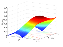
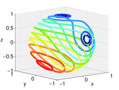
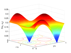
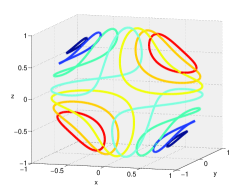
where $\mathfrak{Re}\left(\mathit{Q}\right)$ ($\mathfrak{Im}\left(\mathit{Q}\right)$) is the real (imaginary) part of $\mathit{Q}$, and $\mathit{Q}_{0}$ is given by Eq.(73). In order to study the dependence on the initial conditions, we consider the evolution of pairs of independent states under the QW map. We fix the initial conditions for the first state and study Eq.(95) by considering different points on the Bloch sphere as the initial conditions for the second state. Figures 1 and 2 show our results in two non-equivalent scenarios. As can be seen from these figures, the asymptotic trace distance shows a non trivial behavior as a function of the second state, once the first one is fixed. The left panel can be used to get an idea on how much the trace distance will be reduced (the minimum reduction being of the order of 1/2 in the case represented in Fig. 1, whereas lower values are reached for the parameters that correspond to Fig. 2). In fact, the maximum value of $D(\rho_{12})$ can be shown to be reached when $\rho_{1}$ is defined by $\gamma=0$ and $\rho_{2}$ by $\gamma=\pi$ (or the other way around): That is, when the two states are the North and South poles of the Bloch sphere. As we will discuss later, the same remains true when decoherence is introduced.

The contour levels can be mapped to the points of the Bloch sphere associated to the second state (right panel), thus providing a closer relationship to physical states. As we see by comparing the two figures, changing the first state does not translate into a simple rotation of the Bloch sphere representation, the reason being that the coin operator does not commute with arbitrary rotations.

Figure 1: Left panel: Asymptotic trace distance as a function of the angles $\gamma$ and $\varphi$, representing the initial conditions of $\rho_{2}$. The initial conditions of $\rho_{1}$ are given by $\gamma=0$. Right panel: The contour levels corresponding to to the left panel are mapped to the Bloch sphere, using the same color convention.

Figure 2: Same as Fig. 1, but now the initial conditions for $\rho_{1}$ are given by $\gamma=\pi/4$ and $\varphi=\pi$.

IV Asymptotic density matrix with decoherence

Now we study the dynamics of the reduced density matrix ($\overset{\sim}{\rho_{c}}$) for the QW under the effect of decoherence. For this, we exploit the model of decoherence, known as broken links, that was proposed for the first time in Ref. broken and analyzed in the frame of previous Section in Ref. Mostafa . This model induces decoherence in both degrees of freedom, coin and position. Similar results can be found for other decoherence models.

At each time step $t$, the state of the links in the line is defined. Each link has a probability $p$ of breaking in a given time step. Clearly, for $p=0$, the ideal decoherence-free QW is recovered. During the movement stage, if the walker is in a site with both the links on right and left broken (this happens with probability $p^{2}$), the walker does not move. With probability $(1-p)^{2}$ both links are not broken and, in this case, the evolution normally occurs. With probability $p(1-p)$ only one link is broken and the walker is forced to move to the other direction. Reference Mostafa obtains the superoperator $\mathit{L}_{k}$ that determines the dynamical evolution of the QW with broken links

$$\mathit{L}_{k}=\left(\begin{array}[]{cccc}1&0&0&0\\ 0&0&e&f+p^{2}\\ 0&0&p^{2}-f&e\\ 0&1-2p&-2g&-2h\end{array}\right),$$ (96)

where

$$e = \left(1-p\right)^{2}\sin 2k,$$

$$f = \left(1-p\right)^{2}\cos 2k,$$

$$g = p\left(1-p\right)\sin k,$$

$$h = p\left(1-p\right)\cos k.$$ (97)

The dynamics of the reduced density matrix is again determined by Eq.(57) but now $\mathit{L}_{k}$ is given by Eq.(96). Redefining $\mathit{M}_{k}$ as

$$\mathit{M}_{k}=\left(\begin{array}[]{ccc}0&e&f+p^{2}\\ 0&p^{2}-f&e\\ 1-2p&-2g&-2h\end{array}\right),$$ (98)

it is easy to prove that its eigenvalues $\{\lambda_{i}/i=1,2,3\}$ satisfy $\left|\lambda_{i}\right|<1$ for $p\neq 0$. If $A$ is the matrix constructed from the eigenvectors of the matrix $\mathit{M}_{k}$, and $\Lambda$ the diagonal matrix with the eigenvalues as elements, it is straightforward to prove that

$$\mathit{\lim_{t\rightarrow\infty}M_{k}^{t}} = \lim_{t\rightarrow\infty}(A\Lambda^{t}A^{\dagger})=0.$$ (99)

In this case Eq.(57) gives us

$$\overset{\sim}{\rho}_{c} = \int\limits_{-\pi}^{\pi}\frac{dk}{2\pi}\left(\begin{array}[]{cccc}1&0&0&0\\ 0&0&0&0\\ 0&0&0&0\\ 0&0&0&0\end{array}\right)\left(\begin{array}[]{c}r_{0}\\ r_{1}\\ r_{2}\\ r_{3}\end{array}\right).$$ (108)

In other words, in the formalism of $2\times 2$ matrices, the reduced density matrix in the asymptotic regime is simply

$$\overset{\sim}{\rho_{c}}=\frac{1}{2}\left(\begin{array}[]{cc}1&0\\ 0&1\end{array}\right),$$ (109)

regardless of the initial state. Thus, in the presence of noise, the trace distance of any two different initial states approaches zero, i.e.

$$lim_{t\rightarrow\infty}D(\rho_{12})=0.$$

V Short-time behavior

So far we have investigated the properties of the reduced density matrix in the long-time regime. We obtained a definite limit for both the decoherence-free scenario and the case with decoherence. We now discuss the situation where one considers not the asymptotic limit but a finite number of steps in the QW. Our study, as before, is focused on the time evolution of $D(\rho_{1},\rho_{2})$.

The measure of non-Markovianity given by Ref. Breuer2009 is based on the rate of change of the trace distance

$$\sigma(t,\rho_{1,2}(0))=\frac{d}{dt}D(\rho_{1}(t),\rho_{2}(t)).$$ (110)

Figure 3: Trace distance, as a function of the number of time steps, between the whole density matrices (dashed lines) and between the corresponding reduced density matrices (solid lines). The initial state $\rho_{1}(0)$ is defined by Eq.(9) with $\gamma=0$, while $\rho_{2}(0)$ with $\gamma=\pi$. Different values of the decoherence parameter $p$ have been considered.

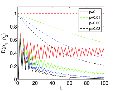
Figure 3 shows the time evolution of the trace distance both for the whole density matrices and for the corresponding reduced density matrices associated with the pair of states giving the maximum trace distance (see below). If one starts from a different pair of states, the curves look qualitatively similar, although the overall scale is smaller.

We have considered various values of the decoherence parameter $p$, the case $p=0$ corresponding to the absence of decoherence. Without decoherence, the QW evolves unitarily, so that the trace distance between two total states is preserved. If $p>0$, the evolution for the total state is clearly Markovian, as indicated by a monotonous decrease in the trace distance (this happens of course for any possible pair of initial states). The reduced density matrices, however, show a completely different behavior. Considering first the case $p=0$, we observe the presence of oscillations, implying that the trace distance increases during some time intervals, giving a positive value of $\sigma$ in Eq. (110). As discussed in Ref. Breuer2009 , this feature is a clear signature of a non-Markovian process. We notice that the amplitude of these oscillations decreases with $t$. For values $p>0$, we also observe the presence of such oscillations. In fact, the curves look similar during the first time steps. However, as $t$ increases the oscillations are more strongly damped than in the decoherence-free case. This effect is even more pronounced for larger values of $p$. In addition to these features, we also notice that the trace distance goes asymptotically to zero, consistently with our results in Sect. IV for the asymptotic limit.

Figure 4: Contribution to the non-Markovianity measure, as a function of the number of time steps, evaluated for the pair of initial states $\rho_{1}(0)$ and $\rho_{2}(0)$ that maximizes the integral in Eq. (111). Different values of the decoherence parameter $p$ have been considered.

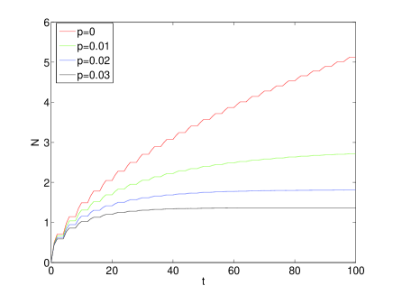
To obtain a quantitative idea about the degree of the non-Markovianity observed in the previous plots, the authors in Ref. Breuer2009 suggest, as a figure of merit, the accumulated area of the trace distance variation for those time intervals where the trace distance is increasing, which amounts to calculating

$$N_{max}=\max_{\rho_{1},\rho_{2}}\int_{\sigma>0}\sigma(\tau,\rho_{1,2}(0))d\tau.$$ (111)

The maximization is performed over all the possible pairs of initial states $\rho_{1}(0)$ and $\rho_{2}(0)$. In our case, due to the fact that we are dealing with a two-level system (the coin), we can restrict our investigation to pairs of orthogonal pure states. Even though, a maximization procedure that takes into account a large time interval is computationally hard. We have checked numerically that the pair of states that maximizes Eq. (111), at least within the time interval $[0,50]$ is the same as in the free case, i.e. the North and South poles of the Bloch sphere. Given its simplicity, we assume that this result holds even for larger time intervals. We have therefore plotted in Fig. 4 the value

$$N(t)=\int_{\sigma>0;\tau\in[0,t]}\sigma(\tau,\rho_{1,2}(0))d\tau,$$ (112)

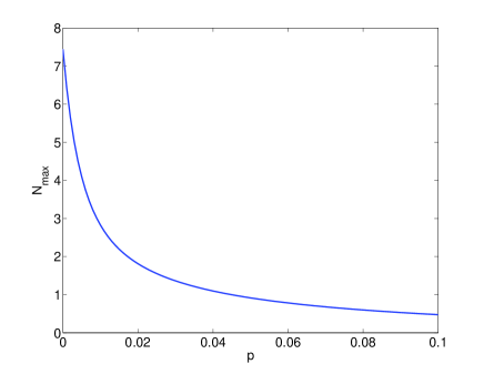
evaluated for this pair of initial states. $N(t)$ can be seen as the contribution to the non-Markovianity measure in the time window $[0,t]$. Even if in the time window allowed by our computational power it is not possible to evaluate (if any) the asymptotic value of $N(t)$ for $t\rightarrow\infty$ (i.e. the non-Markovianity measure $N_{max}$) in the decoherence-free case, the results reported in Fig. 4 give already a very precise picture of how the decoherence affects the degree of non-Markovianity of the coin evolution. This non-Markovianity is stronger as the magnitude of decoherence decreases, with the largest value of its measure corresponding to the decoherence-free case. Fig. 5 shows clearly this feature, where we have plotted the non-Markovianity parameter $N_{max}$ calculated for the time interval $[0,200]$ as a function of $p$, for the North-South pair of states. The curve plotted on this figure can be approximated by the fitting formula $N_{max}(p)\simeq\frac{7.32}{1+150\,p}$.

Figure 5: The non-Markovianity measure, as defined by Eq. (111), calculated for the time interval $[0,200]$ as a function of $p$, for the pair of states that maximizes the final trace distance.

VI Conclusions

In this work we have analyzed both the short-time behavior and the asymptotic limit of the reduced (or chiral) density matrix (i.e. when the spatial degree of freedom is traced out) for the discrete time QW on a one-dimensional lattice. We have found that this reduced system shows clear features which can be associated to a non-Markovian evolution. First, we considered the case where the QW proceeds without decoherence. We observed that the chiral density matrix possesses a well-defined asymptotic limit in time. This allows us to calculate the limiting value of the trace distance for pairs of different initial states.

We have studied the effect of decoherence, modeled as the random presence of broken links on the lattice. The case with decoherence possesses a trivial asymptotic limit, since all states converge to the identity, so that the trace distance between pairs of them always tends to zero.

The short-time behavior of the reduced system features quite interesting results. One observes the presence of oscillations in the trace distance for reduced matrices that correspond to two different initial states, a phenomenon that clearly indicates a non-Markovian time evolution. These oscillations appear even when the system does not suffer from decoherence, and they are damped as the number of time steps increases, thus allowing for a convergence of the trace distance, in accordance with our previous observations. As the level of noise becomes larger, the amplitude of the oscillations is also reduced, for a given number of time steps. In addition, the trace distance approaches asymptotically zero, as already predicted from our long-time analysis. The contribution to the non-Markovianity measure reported in Eq. (111), as a function of the number of time steps, then tends to a value that decreases as the level of decoherence increases.

To conclude, we have found and characterized a non-Markovian behavior for a relatively simple and yet non-trivial system as the coin in a QW on a line. The results that we have presented for the particular model of decoherence chosen here can also be found for other models, as the one investigated in Ref. alejo2013a . They provide a step forward in our understanding of phenomena like the transition from unitary to diffusive processes and of the thermalization of quantum systems, and clearly deserve further attention.