Abstract

We study the quantum properties at one-loop of the Yang-Baxter $\sigma$-models introduced by Klimčík[1, 2]. The proof of the one-loop renormalizability is given, the one-loop renormalization flow is investigated and the quantum equivalence is studied.

Yang-Baxter $\sigma$ model: Quantum aspects

1 Introduction

The Yang-Baxter $\sigma$-models were first introduced by Klimčík [1, 2] as a special case, at the classical level, of a non-linear $\sigma$-model with Poisson-Lie symmetry[3, 4]. Recall that the Poisson-Lie symmetry appears to be the natural generalization of the so-called Abelian $T$-duality[5] and non-Abelian $T$-duality [6, 7, 8] of non-linear $\sigma$-models. In particular, two dynamically equivalent $\sigma$-models can be obtained at the classical level providing that Poisson-Lie symmetry condition holds. That condition takes a very elegant formulation in the case where the target space is a compact semi-simple Lie group which naturally leads to the concept of the Drinfeld double[9]. The Drinfeld double is the $2n$-dimensional linear space where both dynamically equivalent theories live. For the Poisson-Lie $\sigma$-models, a proof of the one-loop renormalizability and quantum equivalence was given in [10, 11, 12, 13].
We are interested by a special class of classical Poisson-Lie $\sigma$-models, the Yang-Baxter $\sigma$-models. Those classical models exhibit the special feature to be both Poisson-Lie symmetric with respect to the right action of the group on itself and left invariant. Thus, using the right Poisson-Lie symmetry or the left group action leads to two different dual theories. Those two dynamically equivalent dual pair of models live in two non-isomorphic Drinfeld doubles, the cotangent bundle of the Lie group for the left action, and the complexified of the Lie group for the right Poisson-Lie symmetry. Classical properties were investigated in the past and it has been showed that Yang-Baxter $\sigma$-models are integrable [1]. More recently, based on the previous work of Refs.[14, 15, 16], authors of Ref.[17] proved that they belong to a more general class of integrable $\sigma$-models. In particular, they showed that the $\varepsilon$-deformation parameter of the Poisson-Lie symmetry can be re-interpreted as a classical $q$-deformation of the Poisson-Hopf algebra.

If classical properties are well investigated, very little is known about the quantum version of the Yang-Baxter $\sigma$-models. In the case where the Lie group is $SU(2)$, the Yang-Baxter $\sigma$-model coincides with the anisotropic principal model which is known to be one-loop renormalizable. This low dimensional result can let us hope a generalization for any Yang-Baxter $\sigma$-models. However, contrary to the anisotropic principal model, the Yang-Baxter $\sigma$-models contain a non-vanishing torsion which could potentially gives rise to some difficulties. On the other hand, another generalization of the anisotropic chiral model, the squashed group models are one-loop renormalizable for a special choice of torsion [22].
Furthermore, the one-loop renormalizability of the Poisson-Lie $\sigma$-model cannot provide any help here since the proof was established for a theory containing $n^{2}$ parameters when the Yang-Baxter $\sigma$-models contain only two: the $\varepsilon$ deformation and the coupling constant $t$. At the quantum level, the Yang-Baxter $\sigma$-models are no more a special case of the Poisson-Lie $\sigma$ models. The main result of this article consists in proving the one-loop renormalizability of Yang-Baxter $\sigma$-models.

The plan of the article is as follows. In Section 2 we introduced the Yang-Baxter $\sigma$-models on a Lie group and all algebraic tools needed. In section 3, the counter-term of the Yang-Baxter $\sigma$-models, i.e. the Ricci tensor, is calculated. Section 4 is dedicated to the proof of the one-loop renormalizability, and the computation of the renormalization flow is done in Section 5. In Section 6, we study the quantum equivalence and we express the Yang-Baxter $\sigma$-action in terms of the usual one of the Poisson-Lie $\sigma$-models. Outlooks take place in Section 7.

2 Yang-Baxter $\sigma$-models

2.1 The complexified double

We considered the case of the Yang-Baxter models studied in Ref.[1]. In that case the Drinfeld double $D$ can be the complexification of a simple compact and simply-connected Lie group $G$, i.e. $D=G^{\mathbb{C}}$, or the cotangent bundle $T^{*}G$. Let us consider the case of the complexified Drinfeld double, it turns out that $D=G^{\mathbb{C}}$ admits the so-called Iwasawa decomposition

$$G^{\mathbb{C}}=GAN=ANG.$$ (1)

In particular, if $D=SL(n,\mathbb{C})$, then the group $AN$ can be identified with the group of upper triangular matrices of determinant $1$ and with positive numbers on the diagonal and $G=SU(n)$.
Furthermore, the Lie algebra ${\cal D}$ turns out to be the complex Lie algebra ${\cal G}^{\mathbb{C}}$, which suggests to use the roots space decomposition of ${\cal G}^{\mathbb{C}}$:

$${\cal G}^{\mathbb{C}}={\cal H}^{\mathbb{C}}\bigoplus(\oplus_{\alpha\in\Delta}\mathbb{C}E_{\alpha}),$$ (2)

where $\Delta$ is the space of all roots. Consider the Killing-Cartan form $\kappa$ on ${\cal G}^{\mathbb{C}}$, and let us take an orthonormal basis $H_{i}$ in the $r$-dimensional Cartan sub-algebra ${\cal H}^{\mathbb{C}}$ of ${\cal G}^{\mathbb{C}}$ with respect to the bilinear form $\kappa$ on ${\cal G}^{\mathbb{C}}$, i.e:

$$\kappa(H_{i},H_{j})\equiv\delta_{ij}$$ (3)

This permits to define a canonical bilinear form on ${\cal H}^{*}$, and more specifically endows the roots space $\Delta\subset{\cal H}^{*}$ with an Euclidean metric, i.e.

$$(\alpha,\beta)=\delta^{ij}\alpha_{i}\beta_{i},\quad\alpha_{i}=\alpha(H_{i}).$$

Moreover, the inner product on the roots space part of ${\cal G}^{\mathbb{C}}$ is chosen such as:

$$\kappa(E_{\alpha},E_{-\alpha})\equiv 1,$$ (4)

and to fix the normalization, we impose the following non-linear condition $E_{\alpha}=E_{-\alpha}^{\dagger}$. With all those conventions, the generators of ${\cal G}^{\mathbb{C}}$ verify:

$$[H_{i},E_{\alpha}]=\alpha_{i}E_{\alpha}\quad [E_{\alpha},E_{-\alpha}]=\displaystyle\alpha^{i}H_{i}$$ (5)

$$[H_{i},H_{j}]=0\quad [E_{\alpha},E_{\beta}]=N_{\alpha,\beta}E_{\alpha+\beta},\;\alpha+\beta\in\Delta.$$

The structure constants $N_{\alpha,\beta}$ vanish if $\alpha+\beta$ is not a root.
Since ${\cal G}^{\mathbb{C}}$ is a Lie algebra, the structure constants verify the Jacobi identity which leads on one hand to:

$$N_{\alpha,\beta}=N_{\beta,-\alpha-\beta}=N_{-\alpha-\beta,\alpha},$$ (6)

and on the other hand to:

$$N_{\alpha,\beta+(k-1)\alpha}N_{\beta+k\alpha,-\alpha}+N_{-\alpha,\beta+(k+1)\alpha}N_{\alpha,\beta+k\alpha}=-(\alpha,\beta+k\alpha).$$ (7)

In the non-vanishing case, the structure constants $N_{\alpha,\beta}$ can be calculated from the last relation

$$N_{\alpha,\beta}^{2}=n(m+1)(\alpha,\alpha),$$ (8)

with $(n,m)\in\mathbb{N}$ such that $\beta+n\alpha$ and $\beta-m\alpha$ are the last roots of the chain containing $\beta$ (see Ref.[21] for more details).
Since $H_{i}$ is an orthonormal basis in ${\cal H}^{\mathbb{C}}$, we obtain the relations:

$$\sum\limits_{\alpha\in\Delta}\alpha_{i}\alpha_{j}=\delta_{ij},\text{ and}\quad\displaystyle\sum\limits_{\alpha\in\Delta}(\alpha,\alpha)=r.$$ (9)

A basis of the compact Lie real form ${\cal G}$ of ${\cal G}^{\mathbb{C}}$ can be obtained by the following transformations:

$$T_{i}=iH_{i},\quad B_{\alpha}=\frac{i}{\sqrt{2}}(E_{\alpha}+E_{-\alpha})\quad C_{\bar{\alpha}}=\frac{1}{\sqrt{2}}(E_{\alpha}-E_{-\alpha}),$$ (10)

with $\alpha\in\Delta^{+}$ (positive roots). With our choice of normalization, the vectors of the basis verify $\kappa(T_{i},T_{j})\equiv\kappa_{ij}=-\delta_{ij}$, $\kappa(B_{\alpha},B_{\beta})\equiv\kappa_{\alpha\beta}=-\delta_{\alpha\beta}$, $\kappa(C_{\bar{\alpha}},C_{\bar{\beta}})\equiv\kappa_{{\bar{\alpha}}{\bar{\beta}}}=-\delta_{\alpha\beta}$ and all others are zero.
Let us define now a $\mathbb{R}$-linear operator $R:{\cal G}\to{\cal G}$ such that:

$$RT_{i}=0,\quad RB_{\alpha}=C_{\bar{\alpha}},\quad RC_{\bar{\alpha}}=-B_{\alpha},$$ (11)

this operator $R$ is the so-called the Yang-Baxter operator [2] which satisfies the following modified Yang-Baxter equation:

$$[RA,RB]=R\big{(}[RA,B]+[A,RB]\big{)}+[A,B],\quad(A,B)\in{\cal G}.$$ (12)

Let us define the skew-symmetric bracket:

$$[A,B]_{R}=[RA,B]+[A,RB],\quad(A,B)\in{\cal G},$$ (13)

which fulfills the Jacobi identity, and defines a new Lie algebra $({\cal G},[.,.]_{R})$. It turns out that this new algebra is nothing but the Lie algebra of the $AN$ group of the Iwasawa decomposition of $G^{\mathbb{C}}$ and will be denoted ${\cal G}_{\mathbb{R}}$ the dual algebra.

2.2 The Yang-Baxter action

We shall now consider the action of the Yang-Baxter $\sigma$-models[2] expressed on the Lie group $G$, which takes the expression:

$${\cal S}(g)=-\frac{1}{2t}\int\kappa\big{(}g^{-1}\partial_{+}g,(\mathbbm{1}-\varepsilon R)^{-1}g^{-1}\partial_{-}g\big{)}d\xi^{+}d\xi^{-},\quad g\in G$$ (14)

where $\partial_{+}=\partial_{\tau}+\partial_{\sigma}$ and $\partial_{-}=\partial_{\tau}-\partial_{\sigma}$, $\mathbbm{1}$ is the identity map on ${\cal G}$, $t$ is the coupling constant and $\epsilon$ is the deformation parameter.
We can immediately check that the Yang-Baxter models (14) are left action invariant, $G$ acting on himself. Concerning the right Poisson-Lie symmetry, it is well known that such $\sigma$-models have to fulfill a zero curvature condition to be Poisson-Lie invariant. Indeed, if we take the following ${\cal G}^{*}$-valued Noether current 1-form $J(g)$:

$$J(g)=-(\mathbbm{1}+\varepsilon R)^{-1}g^{-1}\partial_{+}gd\xi^{+}+(\mathbbm{1}-\varepsilon R)^{-1}g^{-1}\partial_{-}gd\xi^{-},$$ (15)

we can easily verify that the fields equations of (14) are equivalent to the following zero curvature condition:

$$\partial_{+}J_{-}(g)-\partial_{-}J_{+}(g)+\varepsilon[J_{-}(g),J_{+}(g)]_{R}=0.$$ (16)

We remark that if the deformation $\varepsilon$ vanishes then the action of the group $G$ is an isometry, since the Noether current are closed 1-forms on the world-sheets and the action (14) coincides with that of the principal chiral $\sigma$-model.
The operator $(\mathbbm{1}-\varepsilon R)^{-1}$ on ${\cal G}$ can be decomposed in a symmetric part interpreted as a metric $g$ on $G$ and a skew-symmetric part interpreted as a torsion potential $h$ on $G$. An attentive study of the action (14) gives the following expressions for $g$ and $h$:

$$g = \kappa_{ij}(g^{-1}dg)^{i}(g^{-1}dg)^{j}$$ (17)

$$+\frac{1}{1+\varepsilon^{2}}\bigg{(}\kappa_{\alpha\beta}(g^{-1}dg)^{\alpha}(g^{-1}dg)^{\beta}+\kappa_{{\bar{\alpha}}{\bar{\beta}}}(g^{-1}dg)^{\bar{\alpha}}(g^{-1}dg)^{\bar{\beta}}\bigg{)},$$

$$h = -\frac{\varepsilon}{1+\varepsilon^{2}}(g^{-1}dg)^{\alpha}\wedge(g^{-1}dg)^{\bar{\alpha}}\kappa_{\alpha\alpha}.$$ (18)

In order to prove the one-loop renormalizability, we need to calculate the Ricci tensor associated to the manifold $(G,g,h)$.

3 Counter-term of the Yang-Baxter $\sigma$-models

In this paper, for the calculus of the counter-term, we choose the standard approach[18] based on the Ricci tensor. This choice provides a clear and an elegant expression of the counter-term in terms of the roots of $G^{\mathbb{C}}$. However the calculus could have been done by using our formula of [12] for the counter-term in an equivalent way.

3.1 Geometry with torsion on a Lie group $G$

Let us consider a pseudo-Riemannian manifold $(G,g)$ as the base of its frame bundle, where $G$ is a compact semi-simple Lie group and $g$ a non-degenerated metric. Moreover, we choose the left Maurer-Cartan form $g^{-1}dg,\;g\in G$ as the basis of 1-forms on $G$, and in that basis the metric coefficients $g_{ab}$ and the torsion components $T_{abc}$ are all constant.
On that frame bundle we define a metric connection $\Omega$ with its covariant derivative $D$ such that $Dg=0$. Furthermore, if we define by $d^{D}$ the exterior covariant derivative, the torsion can be written $T=d^{D}(g^{-1}dg)$. From these definitions we will obtain the expression of the connection $\Omega$.
Metric connection.
By using the relation $Dg=0$ we obtain:

$$\Omega_{\phantom{a}ac}^{s}g_{sb}+\Omega^{s}_{\phantom{b}bc}g_{as}=0.$$ (19)

With $g_{ab}$ constant and if we denote $\Omega_{abc}=g_{as}\Omega^{s}_{\phantom{a}bc}$, the previous relation becomes:

$$\Omega_{abc}=-\Omega_{bac}$$ (20)

Thus the two first indices of the connection $\Omega$ are skew-symmetric.
The torsion.
We said that the torsion verifies $T=d^{D}(g^{-1}dg)$ or in terms of components:

$$T^{a}=\Omega^{a}_{\phantom{a}b}\wedge(g^{-1}dg)^{b}+d(g^{-1}dg)^{a}.$$ (21)

Since $g^{-1}dg$ is the left Maurer-Cartan form on ${\cal G}$, we get:

$$d(g^{-1}dg)=-(g^{-1}dg)\wedge(g^{-1}dg),$$

on the other hand $T^{a}$ is the 2-form torsion, i.e. we can write it as:

$$T^{a}=\frac{1}{2}T^{a}_{\phantom{b}bc}(g^{-1}dg)^{b}\wedge(g^{-1}dg)^{c}.$$

Consequently, the components of the torsion are related to the skew-symmetric part of the connection as:

$$T^{a}_{\phantom{a}bc}=\Omega^{a}_{\phantom{b}cb}-\Omega^{a}_{\phantom{b}bc}-f^{\phantom{bc}a}_{bc},$$ (22)

with $f^{\phantom{bc}a}_{bc}$ the structure constants of the Lie algebra ${\cal G}$.
Note that in the case of the non-linear $\sigma$-models the torsion is defined by $T=dh$ where $h$ is the 2-form potential torsion, we will exploit that a little further to express the connection for the Yang-Baxter $\sigma$-models.
The connection.
From the relations (20)(22), we can find the components of the connection:

$$2\Omega_{abc}=(-T_{abc}-T_{bca}+T_{cab})+(f_{abc}-f_{cab}-f_{bca}),$$ (23)

with the conventions $\Omega_{abc}=g_{as}\Omega^{s}_{\phantom{b}bc}$, $T_{abc}=g_{as}T^{s}_{\phantom{a}bc}$ and $f_{bca}=f^{\phantom{ab}s}_{bc}g_{sa}$.
Let us introduce the Levi-Civita connection $L$ which is in fact the second term of the r.h.s in Eq.(23), and rewrite the connection $\Omega$ for a totally skew-symmetric torsion:

$$\Omega_{abc}=L_{abc}-\frac{1}{2}T_{abc}.$$ (24)

The curvature and the Ricci.
By definition the 2-form curvature $F$ fulfills $F=d^{D}\Omega$, i.e.

$$F^{a}_{\phantom{a}b}=d\Omega^{a}_{\phantom{a}b}+\Omega^{a}_{\phantom{a}s}\wedge\Omega^{s}_{\phantom{a}b}.$$ (25)

Moreover, since $\Omega^{a}_{\phantom{a}b}$ is a 1-form of $G$, $\Omega^{a}_{\phantom{a}b}=\Omega^{a}_{\phantom{a}bc}(g^{-1}dg)^{c}$, we obtain the general expression for the curvature:

$$F^{a}_{\phantom{a}bcd}=\Omega^{a}_{\phantom{a}sc}\Omega^{s}_{\phantom{a}bd}-\Omega^{a}_{\phantom{a}sd}\Omega^{s}_{\phantom{a}bc}-\Omega^{a}_{\phantom{a}bs}f^{s}_{cd}.$$ (26)

The Ricci tensor is such that $Ric_{ab}=F^{s}_{\phantom{a}asb}$ and can be written as:

$$Ric_{ab}=-\Omega^{s}_{\phantom{ab}ar}(\Omega^{r}_{\phantom{ab}bs}+f^{r}_{\phantom{ab}bs}).$$ (27)

We are now able to decompose the symmetric and skew-symmetric parts of the Ricci tensor in terms of the torsion-less Ricci tensor $Ric^{L}$ and the torsion $T$ as:

$$Ric_{(ab)}=Ric_{(ab)}^{L}+\frac{1}{4}T^{r}_{\phantom{a}as}T^{s}_{\phantom{a}br}$$ (28)

$$Ric_{[ab]}=\frac{1}{2}f_{at}^{\phantom{ab}s}T^{t}_{\phantom{a}bs}-\frac{1}{2}g_{at}f_{sr}^{\phantom{ab}t}g^{ru}T^{s}_{\phantom{a}bu}+\frac{1}{2}g_{st}f_{ar}^{\phantom{ab}t}g^{ru}T^{s}_{\phantom{a}bu}-(a\leftrightarrow b).$$ (29)

3.2 Application to Yang-Baxter

Ricci symmetric part

:
Recall that in the case of the Yang-Baxter $\sigma$-models and with our normalization choice, the metric is given by:

$$g_{ij}=-\delta_{ij},\quad g_{\alpha\beta}=-\frac{1}{1+\varepsilon^{2}}\delta_{\alpha\beta},\quad g_{{\bar{\alpha}}{\bar{\beta}}}=-\frac{1}{1+\varepsilon^{2}}\delta_{\alpha\beta}.$$ (30)

Let us introduce the bi-invariant connection $\Gamma$ on the Lie group $G$, it corresponds to the Levi-Civita connection in the case of a vanishing deformation, i.e. $\Gamma=L(\varepsilon=0)$. From the equations (23) we can obtain the Levi-Civita coefficients:

$$L^{\alpha}_{\phantom{a}{\bar{\alpha}}i}=-L^{\bar{\alpha}}_{\phantom{a}\alpha i}=(1-\varepsilon^{2})\Gamma^{\alpha}_{\phantom{a}{\bar{\alpha}}i}$$ (31)

$$L^{\alpha}_{\phantom{a}i{\bar{\alpha}}}=-L^{\bar{\alpha}}_{\phantom{a}i\alpha}=(1+\varepsilon^{2})\Gamma^{\alpha}_{\phantom{a}i{\bar{\alpha}}},$$ (32)

where we keep the convention for the indices $i\in{\cal H}$ and $\alpha\in\Delta^{+}$. All others Levi-Civita coefficients are equal to those of the bi-invariant connection $\Gamma$.
We can now express the torsion-less Ricci tensor $Ric^{L}$ as a deformation of the usual Ricci tensor $Ric^{\Gamma}$ of the bi-invariant connection on Lie group, i.e.

$$Ric^{L}_{\phantom{a}\alpha\beta} = Ric^{\Gamma}_{\alpha\beta}-\frac{\varepsilon^{2}}{2}(\alpha,\alpha)\delta_{\alpha\beta}$$ (33)

$$Ric^{L}_{\phantom{a}{\bar{\alpha}}{\bar{\beta}}} = Ric^{\Gamma}_{{\bar{\alpha}}{\bar{\beta}}}-\frac{\varepsilon^{2}}{2}(\alpha,\alpha)\delta_{\alpha\beta}$$ (34)

$$Ric_{\phantom{a}ij}^{L} = (1+\varepsilon^{2})^{2}Ric^{\Gamma}_{\phantom{a}ij}$$ (35)

It is well-known that for the Riemannian bi-invariant structure the Ricci tensor takes the expression:

$$Ric^{\Gamma}_{ab}=-\frac{1}{4}\kappa_{ab},\quad(a,b)\in G,$$ (36)

therefore, the components of $Ric^{L}$ are the following:

$$Ric^{L}_{\phantom{a}\alpha\beta} = Ric^{L}_{\phantom{a}{\bar{\alpha}}{\bar{\beta}}}=-\frac{1}{4}\kappa_{\alpha\beta}-\frac{\varepsilon^{2}}{2}(\alpha,\alpha)\delta_{\alpha\beta}$$ (37)

$$Ric_{\phantom{a}ij}^{L} = -\frac{1}{4}\kappa_{ij}(1+\varepsilon^{2})^{2}$$ (38)

Concerning the contribution of the Torsion to the symmetric part of the Ricci tensor, we have to express the Torsion in terms of the constant structures of $G$. For a non-linear $\sigma$-model the Torsion $3$-form is calculated from the potential torsion $2$-form such $T=dh$, which implies that:

$$T_{abc}=-3f^{\phantom{ab}s}_{[ab}h_{c]s},\quad(a,b,c,s)\in G.$$ (39)

Moreover, since the torsion potential involves only root indices

$$h=-\frac{\varepsilon}{1+\varepsilon^{2}}(g^{-1}dg)^{\alpha}\wedge(g^{-1}dg)^{\bar{\alpha}}\kappa_{\alpha\alpha},$$

the torsion components vanish for the Cartan sub-algebra indices ($T_{ibc}=0$).
We can now calculate the torsion contribution, and we obtain for the non-vanishing coefficients:

$$\frac{1}{4}T^{r}_{\phantom{a}\alpha s}T^{s}_{\phantom{a}\alpha r}=\frac{1}{4}T^{r}_{\phantom{a}{\bar{\alpha}}s}T^{s}_{\phantom{a}{\bar{\alpha}}r}=\frac{\varepsilon^{2}}{2}\big{(}\frac{1}{2}\kappa_{\alpha\alpha}+(\alpha,\alpha)\big{)}.$$ (40)

In the calculus we used the fact that the Killing $\kappa$ can be expressed in terms of the root $\alpha$ and the constant structures $N_{\alpha,\beta}$ such as:

$$-\frac{1}{2}\kappa_{\alpha\alpha}=\alpha^{i}\alpha_{i}+\frac{1}{2}\sum_{\beta\in\Delta^{+}}(N_{\alpha,\beta})^{2}+(N_{\alpha,-\beta})^{2}.$$ (41)

Adding both contributions to the Ricci tensor and using our normalization, we obtain the final expression of the symmetric part:

$$Ric_{\alpha\beta}=Ric_{{\bar{\alpha}}{\bar{\beta}}}=-\frac{\kappa_{\alpha\beta}}{4}(1-\varepsilon^{2})=\frac{1}{4}(1-\varepsilon^{2})\delta_{\alpha\beta}$$ (42)

$$Ric_{ij}=-\frac{\kappa_{ij}}{4}(1+\varepsilon^{2})^{2}=\frac{\delta_{ij}}{4}(1+\varepsilon^{2})^{2}.$$ (43)

We observe that, in the case of the Yang-Baxter model, the torsion induced by the Poisson-Lie symmetry is precisely that which avoids the dependence of the Ricci tensor in the root length $(\alpha,\alpha)$.

Ricci skew-symmetric part

:
Using the fact the $T_{iab}=0$, the only non-vanishing non-diagonal components of the Ricci tensor can be written:

$$Ric_{\alpha{\bar{\alpha}}}=2f_{\alpha{\bar{\beta}}\gamma}T_{{\bar{\alpha}}{\bar{\beta}}\gamma}\kappa^{\gamma\gamma}\kappa^{{\bar{\beta}}{\bar{\beta}}}-f_{{\bar{\alpha}}\beta\gamma}T_{\alpha\beta\gamma}\kappa^{\gamma\gamma}\kappa^{\beta\beta}-f_{{\bar{\alpha}}{\bar{\beta}}{\bar{\gamma}}}T_{\alpha{\bar{\beta}}{\bar{\gamma}}}\kappa^{{\bar{\gamma}}{\bar{\gamma}}}\kappa^{{\bar{\beta}}{\bar{\beta}}}.$$ (44)

The first r.h.s term can be expressed as a function of the structure constants, $N_{\alpha,\beta}$ such as:

$$2f_{\alpha{\bar{\beta}}\gamma}T_{{\bar{\alpha}}{\bar{\beta}}\gamma}\kappa^{\gamma\gamma}\kappa^{{\bar{\beta}}{\bar{\beta}}}=2\varepsilon\sum_{\beta\in\Delta^{+}}(N_{\alpha,\beta})^{2}-(N_{\alpha,-\beta})^{2}.$$ (45)

The two other terms are nothing but the contribution of the roots space (see Eq.(41)) to the component $\kappa_{{\bar{\alpha}}{\bar{\alpha}}}$ of the Killing form, i.e.:

$$-f_{{\bar{\alpha}}\beta\gamma}T_{\alpha\beta\gamma}\kappa^{\gamma\gamma}\kappa^{\beta\beta}-f_{{\bar{\alpha}}{\bar{\beta}}{\bar{\gamma}}}T_{\alpha{\bar{\beta}}{\bar{\gamma}}}\kappa^{{\bar{\gamma}}{\bar{\gamma}}}\kappa^{{\bar{\beta}}{\bar{\beta}}}=-\frac{\varepsilon}{2}\bigg{(}\kappa_{{\bar{\alpha}}{\bar{\alpha}}}+2(\alpha,\alpha)\bigg{)}.$$ (46)

By summing the Bianchi relations (7) on positive roots, we obtain that:

$$\sum_{\beta\in\Delta^{+}}(N_{\alpha,\beta})^{2}-(N_{\alpha,-\beta})^{2}=-2(\rho,\alpha)+(\alpha,\alpha),$$ (47)

with

$$\rho=\frac{1}{2}\sum_{\alpha\in\Delta^{+}}\alpha$$

the Weyl vector.
Finally, the skew-symmetric part of the Ricci tensor is given by:

$$Ric_{\alpha{\bar{\alpha}}}=-Ric_{{\bar{\alpha}}\alpha}=-\varepsilon\bigg{(}2(\alpha,\rho)+\frac{1}{2}\kappa_{\alpha\alpha}\bigg{)}.$$ (48)

4 One-loop renormalizability

At one-loop the counter-terms for a non-linear $\sigma$-model[18] on $G$ are given by:

$$\frac{1}{4\pi\epsilon}\int Ric_{ab}(g^{-1}\partial_{-}g)^{a}(g^{-1}\partial_{+}g)^{b},\quad\epsilon=2-d.$$ (49)

We require, for the renormalizability, that all divergences have to be absorbed by fields-independent deformations of the parameters $(t,\varepsilon)$ and a possible non-linear fields renormalization of the fields $(g^{-1}\partial_{\pm}g)^{a}$. Thus, if we suppose that all parameters are the independent coupling constants of the theory, the Ricci tensor in our frame has to verify the relations:

$$Ric_{ab}=-\chi_{0}(\mathbbm{1}-\varepsilon R)^{-1}_{ab}+\chi_{\varepsilon}\frac{\partial}{\partial\varepsilon}(\mathbbm{1}-\varepsilon R)^{-1}_{ab}+D_{b}u_{a},$$ (50)

with $u$ a vector that contributes to the fields renormalization, $\chi_{0}$ and $\chi_{\varepsilon}$ are coordinates-independent. Decomposing into symmetric and skew-symmetric parts, the previous relation for the Yang-Baxter $\sigma$-models becomes:

$$Ric_{ij} = -\chi_{0}g_{ij}$$ (51)

$$Ric_{\alpha\alpha} = -\chi_{0}g_{\alpha\alpha}-\chi_{\varepsilon}\frac{2\varepsilon}{1+\varepsilon^{2}}g_{\alpha\alpha}$$ (52)

$$Ric_{\alpha{\bar{\alpha}}} = -\chi_{0}h_{\alpha{\bar{\alpha}}}+\chi_{\varepsilon}\frac{1-\varepsilon^{2}}{\varepsilon(1+\varepsilon^{2})}h_{\alpha{\bar{\alpha}}}+D_{{\bar{\alpha}}}u_{\alpha}.$$ (53)

From the equations (51) and (52), we extract immediately:

$$\chi_{0}=\frac{1}{4}(1+\varepsilon^{2})^{2},\textrm{ and }\;\chi_{\varepsilon}=-\frac{1}{4}\varepsilon(1+\varepsilon^{2})^{2}.$$ (54)

Since $\chi_{0}$ and $\chi_{\varepsilon}$ are now fixed, they have to fulfill in the same time the relation (53), which gives the following constraint:

$$\varepsilon\bigg{(}-\frac{1}{2}+2(\rho,\alpha)\bigg{)}=-\frac{1}{2}\varepsilon+D_{{\bar{\alpha}}}u_{\alpha}.$$ (55)

Furthermore, the covariant derivative of $u$ can be easily calculated:

$$Du=-\frac{1}{2}\sum_{\alpha\in\Delta^{+}}(u,\alpha)(g^{-1}dg)^{\alpha}\wedge(g^{-1}dg)^{\bar{\alpha}}.$$ (56)

Let us define the vector $\varepsilon\bar{u}=u$, and insert (56) in the constraint (55) we obtain:

$$(4\rho-\bar{u},\alpha)=0.$$ (57)

Then, if we impose $\bar{u}=4\rho$ the constraint is fulfilled for any root $\alpha$ since $(.,.)$ is the canonical scalar product on ${\mathbb{R}}^{r}$ . We can conclude that the Yang-Baxter $\sigma$-models are one-loop renormalizable.
We note that it is quite elegant to find a field renormalization given by the Weyl vector.

5 Renormalization flow

Let us introduce the $\beta$-functions of the two parameters $(t,\varepsilon)$, they satisfy:

$$\beta_{t}=\frac{dt}{d\lambda}=-t^{2}\chi_{0},\quad\beta_{\varepsilon}=\frac{d\varepsilon}{d\lambda}=t\chi_{\varepsilon},$$ (58)

where $\lambda=\frac{1}{\pi}\ln\mu$, with $\mu$ the mass energy scale. We obtain the following system of differential equations:

$$\frac{dt}{d\lambda}+\frac{1}{4}(1+\varepsilon^{2})^{2}t^{2} = 0$$ (59)

$$\frac{d\varepsilon}{d\lambda}+\frac{1}{4}\varepsilon(1+\varepsilon^{2})^{2}t = 0.$$ (60)

The set of differential equations can be exactly solved, and solutions take the following general expressions:

$$t(\varepsilon)=A\varepsilon,\quad\hat{\lambda}(\varepsilon)=B\lambda(\varepsilon)=\frac{3}{2}\arctan\varepsilon+\frac{1+\frac{3}{2}\varepsilon^{2}}{\varepsilon(1+\varepsilon^{2})^{2}}+C,$$ (61)

with $(A,B,C)\in{\mathbb{R}}$ three integrative constants. We note that divergences occur for $\varepsilon$ and $t$ when the energy scale $\hat{\lambda}$ goes to $\pm\frac{3\pi}{4}+C$. On the other hand, for $\hat{\lambda}\to\infty$ the parameters $\varepsilon$ and $t$ are vanishing, leading to an asymptotic freedom. We can illustrate the situation with the following plot (Fig.1) of $\lambda$ as a function of $\varepsilon$ where we choose $B=1$ and $C=0$.

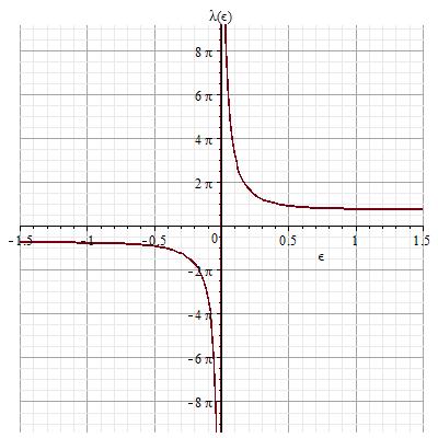
Figure 1: Energy scale $\lambda$ as a function of the deformation parameter $\varepsilon$

6 Poisson-Lie models and duality

Now we will express the Yang-Baxter $\sigma$-models in terms of the usual Poisson-Lie $\sigma$-models’ expression. Recall that general Right symmetric Poisson-Lie $\sigma$-models can be written:

$$\mathcal{S}(g)=\frac{1}{2\tilde{t}}\int(\partial_{-}gg^{-1})^{a}(M+\Pi_{R}(g))^{-1}_{ab}(\partial_{+}gg^{-1})^{b}.$$ (62)

Here $\Pi_{R}(g)$ is the so-called Right Poisson-Lie bi-vector and $M$ an $n^{2}$ real matrix.
Using the adjoint action of an element $g\in G$ we can rewrite the action (14) such as the previous (62), with

$$\Pi_{R}(g)=\mathrm{Ad}_{g}R\mathrm{Ad}_{g^{-1}}-R\textrm{ and }M=\frac{1}{\varepsilon}\mathbbm{1}-R.$$

Let us focus on the dual models, as evoked earlier there exists two non-isomorphic Drinfeld doubles for the action (62). Consequently, we have two different dual theories for one single initial theory on $G$, and all three are classically equivalent. We will consider each case and argue that they are all quantum-equivalent at one-loop.
We start by considering the Drinfeld double $D=G^{\mathbb{C}}$, in that case we saw that the dual group is the factor $AN$ in the Iwasawa decomposition. The corresponding algebra is the Lie algebra ${\cal G}_{\mathbb{R}}$ generated by the ${\mathbb{R}}$-linear operator $(R-i)$ on ${\cal G}$, whose its group is a non-compact real form of $G^{\mathbb{C}}$ (see [2, 20] for details). The dual action can be expressed as:

$$\mathcal{S}(\hat{g})=\frac{1}{2\varepsilon t}\int(\partial_{-}\hat{g}\hat{g}^{-1})_{a}\big{[}(M^{-1}+\hat{\Pi}_{R}(\hat{g}))^{-1}\big{]}^{ab}(\partial_{+}\hat{g}\hat{g}^{-1})_{b}.$$ (63)

K.Sfetsos and K.Siampos proved in [10] that for Right Poisson-Lie symmetric $\sigma$-models the quantum equivalence holds providing that the matrix $M$ is invertible. In the Yang-Baxter $\sigma$-models this condition is always satisfied and the inverse of $M$ is given by:

$$M^{-1}=\frac{\varepsilon^{2}}{1+\varepsilon^{2}}\left(\frac{1}{\varepsilon}\,\mathbbm{1}+R\right)$$

.
When we consider the dual model associated to the left action of $G$, the Drinfeld double is the cotangent bundle $T^{*}G=G\ltimes{\cal G}^{*}$. Then the dual group is the dual linear space ${\cal G}^{*}$ of ${\cal G}$, which is an Abelian group with the addition of vectors as the group law. The corresponding action is that of the non-Abelian $T$-dual $\sigma$-models [6, 7, 8] and has the well-known expression:

$$\mathcal{S}(\hat{g}=e^{s\chi})=\frac{1}{2\varepsilon t}\int d\xi^{+}d\xi^{-}\partial_{-}\chi_{a}\big{(}(M^{-1})_{ab}+f_{ab}^{c}\chi_{c}\big{)}^{-1}\partial_{+}\chi_{b},\;\chi\in{\cal G}^{*},\;s\in{\mathbb{R}}.$$ (64)

It has been showed in [19] that those models are one-loop renormalizable. Since the action (64) is Left Poisson-Lie symmetric, Sfetsos-Siampos condition [10] still holds (in their Left formulation) and implies again the quantum equivalence at one-loop.

7 Outlooks

Yang-Baxter $\sigma$-models are one case of non-trivial Poisson-Lie symmetric $\sigma$-models which keep the renormalizability and the quantum equivalence at the one-loop level, and are known to be classically integrable. Those models appear to be a semi-classical $q$-deformation of Poisson algebra, and can be a starting point in the quest for a quantum $q$-deformation fully renormalizable thanks to the relative simplicity of these models containing only two parameters .
Furthermore, for low dimensional compact Lie groups $G$ the geometry associated to the Yang-Baxter $\sigma$-models can be viewed as a torsionless Einstein-Weyl geometry. We plan in the future to study the Weyl connections with torsion on Einstein manifolds, with the hope to learn more about the geometric aspects of the Poisson-Lie $\sigma$-models.

I thank G.Valent for discussions and C.Carbone for proofreading.

References

• [1] C. Klimฤรญk, Yang-Baxter $\sigma$-models and dS/AdS T-duality, JHEP 0212 (2002) 051, hep-th/0210095
• [2] C. Klimฤรญk, On integrability of the Yang-Baxter $\sigma$-model, J.Math.Phys. 50:043508,2009, hep-th/08023518.
• [3] C. Klimฤรญk and P. ล evera, Dual Non-Abelian Duality and the Drinfeld Double, Phys.Lett.B351 (1995) 455-462, hep-th/9502122
• [4] C. Klimฤรญk and P. ล evera, Poisson-Lie T-duality and Loop Groups of Drinfeld Doubles, Phys.Lett. B372 (1996) 65-71, hep-th/9512040
• [5] K. Kikkawa, M. Yamasaki, Phys. Lett. B 149 (1984) 357;
N. Sakai, I. Senda, Prog. Theor. Phys. 75 (1986) 692.
• [6] X. de la Ossa and F. Quevedo, Nucl. Phys. B403 (1993) 377.
• [7] B.E. Fridling, A. Jevicki, Phys. Lett. B 134 (1984) 70.
• [8] E.S. Fradkin, A.A. Tseytlin, Ann. Phys. 162 (1985) 31.
• [9] V.G. Drinfeld, Quantum Groups, in Proc. ICM, MSRI, Berkeley (1986) p. 708;
F. Falceto, K. Gawศฉdzki, J. Geom. Phys. 11 (1993) 251;
A.Yu. Alekseev, A;Z. Malkin, Commun. Math. Phys. 162 (1994) 147.
• [10] Konstadinos Sfetsos, Konstadinos Siampos Quantum equivalence in Poisson-Lie T-duality , JHEP 0906 (2009) 082, hep-th/0904.4248.
• [11] K. Sfetsos, Phys. Lett. B 432 (1998) 365.
• [12] G. Valent, C. Klimฤรญk, R. Squellari, One loop renormalizability of the Poisson-Lie $\sigma$-models, Phys. Lett. B678 (2009) 143-148, hep-th/0902.1459.
• [13] K. Sfetsos, K. Siampos, Daniel C. Thompson, Renormalization of Lorentz non-invariant actions and manifest T-duality, Nucl.Phys.B827:545-564, 2010.
• [14] I. Kawaguchi and K. Yoshida, Hybrid classical integrability in squashed sigma models, Phys. Lett. B705 (2011) 251โ€“254, [arXiv:1107.3662].
• [15] I. Kawaguchi, T. Matsumoto, and K. Yoshida, On the classical equivalence of monodromy matrices in squashed sigma model, JHEP 1206 (2012) 082, [arXiv:1203.3400].
• [16] Io Kawaguchi, Takuya Matsumoto, Kentaroh Yoshida, The classical origin of quantum affine algebra in squashed sigma models, 10.1007/JHEP04(2012)115, hep-th/1201.3058
• [17] Francois Delduc, Marc Magro, Benoit Vicedo, On classical q-deformations of integrable sigma-models, hep-th/1308.3581. (2013)
• [18] B. E. Friedling and A. E. M. Van de Ven, Nucl. Phys. B 268 (1986) 719.
• [19] P. Y. Casteill, G. Valent Quantum structure of T-dualized models with symmetry breaking, Nucl.Phys. B591 (2000) 491-514 , hep-th/0006186.
• [20] C.Klimฤรญk, Quasitriangular WZW model, Rev. Math. Phys. 16 (2004) 679-808, hep-th/0103118.
• [21] Robert Gilmore, Lie Groups, Lie Algebras, and Some of Their Applications, ISBN 0-486-44529-1, 2006.
• [22] Dan Israรซl, Costas Kounnas, Domenico Orlando, and P. Marios Petropoulos Heterotic strings on homogeneous spaces Fortsch. Phys. 53 (2005) 1030-1071, hep-th/0412220.