Realization of quantum gates by Lyapunov control

Abstract

We propose a Lyapunov control design to achieve specific (or a family of) unitary time-evolution operators, i.e., quantum gates in the Schrödinger picture by tracking control. Two examples are presented. In the first, we illustrate how to realize the Hadamard gate in a single-qubit system, while in the second, the controlled-NOT (CNOT) gate is implemented in two-qubit systems with the Ising and Heisenberg interactions. Furthermore, we demonstrate that the control can drive the time-evolution operator into the local equivalence class of the CNOT gate and the operator keeps in this class forever with the existence of Ising coupling.

1 Introduction

Quantum information processing [1] has become an interdisciplinary research field covering the investigation of fundamental questions in quantum physics [2], metrology [3, 4] as well as the quest for a quantum computer. The Hadamard gate and the Controlled-NOT (CNOT) gate are the building blocks for quantum computing, which can be realized by quantum control [5, 6]. Various techniques have been developed for quantum control [7, 8, 9, 10, 11, 12, 13, 14], which can be divided into coherent and in-coherent ones. Quantum coherent optimal control is a powerful tool for designing control fields, although finding the control fields is a time-consuming task. Recently, it has found applications in many problems [7, 8, 15, 16, 17, 18, 19, 20, 21].

Quantum Lyapunov control was proposed as a good candidate for quantum state engineering. It has been well developed in both theory and applications in the last decades [14, 22, 23, 24, 25, 26, 27, 28, 29, 30, 31]. The authors in Ref. [22, 23, 24, 25, 30, 31] investigated different types of Lyapunov functions, schemes of field design and their convergence. In Ref. [26, 27, 28], Lyapunov control was applied to driving an open quantum system to its decoherence-free subspace, preparing entanglement states, and enforcing adiabatic evolutions.

In quantum Lyapunov control, the control fields are designed to make the Lyapunov function decrease monotonically, while the system is asymptotically steered to a desired state. The total Hamiltonian of the system under control takes the form $H_{0}+\sum_{n}f_{n}(t)H_{n}$, where $H_{0}$ is the free Hamiltonian which can usually not be turned off. $H_{n}$ stand for the external control Hamiltonians with $f_{n}(t)$ the corresponding control fields. Lyapunov control can be understood as a local optimization [32] with the control fields determined at every instant of time in feedback form. Similar to quantum coherent optimal control, Lyapunov control can be used to deal with different forms of Hamiltonian systems. However, the calculation of control fields for Lyapunov control is much easier since it does not need iteration. Another merit of Lyapunov control is that the shape of control fields is flexible [29].

Lyapunov control is mostly used to prepare quantum states. This method can be extended to produce unitary operators (quantum gates) in view of its advantages. Sklarz and Tannor studied the creation of quantum gates in the subspace of a direct sum or direct product Hilbert space by local-in-time control (Lyapunov control) working in the interaction picture with respect to $H_{0}$ [14]. However, in the presence of the free Hamiltonian $H_{0}$, the time-evolution operator can usually not reach a stationary one in the Schrödinger picture. Our goal in this letter is to prepare desired time-evolution operators in the Schrödinger picture by Lyapunov control such that quantum gates might be easier to realize in the laboratory frame. We use a tracking strategy for engineering time-evolution operators. The Lyapunov function is designed to be a distance between the time-evolution operator $U$ and $e^{-iH_{0}t}O$, where $O$ is the target quantum gate. In this way, the control fields can steer $U$ to the orbit (defined in Section 2) of $e^{-iH_{0}t}O$, such that the time-evolution operator might reach $O$ at particular instances of time, or stays in a desired family of operators forever. Note that tracking the time-dependent operator $e^{-iH_{0}t}O$ in the Schrödinger picture is equivalent to tracking $O$ in the interaction picture. However, if $U_{I}(t)\rightarrow O$ in the interaction frame, the evolution operator $U(t)$ in the Schrödinger picture is generally not $O$ and the gate time $t_{g}$ with $U(t_{g})=O$ is not clear. Therefore, it is more convenient to calculate the field in the Schrodinger picture.

The letter is organized as follows. We present in Section 2 the Lyapunov function and the design of control fields based on a tracking strategy. In Section 3.1, we demonstrate the implementation of the Hadamard gate with a typical single-qubit Hamiltonian. In Section 3.2, the CNOT gate is realized in two-spin systems with the Ising and Heisenberg interactions. We show further in Section 4 that the time-evolution operator can stay in the local equivalence class of the CNOT gate forever with the same control as in Section 3.2. This is the main difference between the present Lyapunov control and the other strategies discussed in the literature [8, 9, 18, 19, 20, 21] where the aimed quantum gate is obtained at a fixed time. Finally, we summarize our work in Section 5.

2 General theory

Our task is to design control fields to realize a target quantum gate (or a desired family of quantum gates) by Lyapunov control in a closed system. The dynamical equation for the time-evolution operator $U$ is

$$i\frac{dU}{dt}=(H_{0}+\sum_{n}f_{n}(t)H_{n})U,$$ (1)

where $H_{0}$ is the free Hamiltonian and $H_{n}$ $(n=1,2,3,...)$ are the control Hamiltonians with $f_{n}(t)$ the control fields. At the initial time, $U(0)=\text{I}$ where I is the identity operator. For simplicity, we set $\hbar=1$ throughout this letter. We restrict our discussion to finite dimensional quantum systems where all the operators can be represented by $N\times N$ matrices.

If the time-evolution operator $U$ is driven to $O$ (the target operator) with all the control fields being turned off, $U$ will evolve as $U(t)=e^{-iH_{0}t}O$ which is usually different from $O$ at a later time. To be specific, consider an $N$-dimensional system in the space spanned by the eigenstates of $H_{0}$ which is written as $H_{0}=diag\{\lambda_{1},\lambda_{2},...\lambda_{N}\}$. Then the time-evolution operator $U(0)=O$ governed by $H_{0}$ evolves as

$$U(t) = e^{-iH_{0}t}O$$

$$= \left(\begin{array}[]{cccc}e^{-i\lambda_{1}t}O_{11}&e^{-i\lambda_{1}t}O_{12}&\cdots&e^{-i\lambda_{1}t}O_{1N}\\ e^{-i\lambda_{2}t}O_{21}&e^{-i\lambda_{2}t}O_{12}&\cdots&e^{-i\lambda_{2}t}O_{2N}\\ &&\cdots&\\ e^{-i\lambda_{N}t}O_{N1}&e^{-i\lambda_{N}t}O_{N2}&\cdots&e^{-i\lambda_{N}t}O_{NN}\\ \end{array}\right),$$

where $O_{ij}$ $(i,j=1,2\cdots N)$ are the elements of the unitary operator $O$. Clearly $U(t)$ evolves under $H_{0}$ except the trivial case, $\lambda_{1}=\lambda_{2}=...=\lambda_{N}$. Therefore, one can not asymptotically steer the system to a target operator $O$ as $t\rightarrow\infty$. Instead, we use a tracking strategy to steer the time-evolution operator $U$ to track the evolving operator

$$\tilde{O}(t)=e^{-iH_{0}t}O.$$ (7)

Once $U\rightarrow\tilde{O}(t)$ or evolves into the orbit of $\tilde{O}(t)$, $U$ is expected to reach $O$ at later times. Here, the orbit of $\tilde{O}(t)$ is defined as a set of operators, $S=\{U|U=e^{-iH_{0}T}\tilde{O}(t),T\in\mathbf{R}\}=\{U|U=e^{-iH_{0}T}O,T\in\mathbf{R}\}$. It is evident that the orbit of $\tilde{O}(t)$ is also the orbit of $O$.

The Lyapunov function here is based on the fidelity of two unitary matrices

$$F=\frac{|\text{Tr}(U_{1}^{{\dagger}}U_{2})|}{N},$$ (8)

where $N=\text{Tr}(U_{1}^{{\dagger}}U_{1})$ is the dimension of the system. The fidelity is often used to measure the difference between two unitary operators [8, 33, 34]. If $F=1$, $U_{1}$ and $U_{2}$ are equal up to a non-physical global phase. With these notations, we define the Lyapunov function as

$$V=1-\frac{1}{N^{2}}|\text{Tr}(\tilde{O}^{{\dagger}}(t)U)|^{2},$$ (9)

which can be understood as a distance between $U$ and $\tilde{O}(t)$ [35]. The function satisfies $0\leq V\leq 1$. If $U=e^{i\theta}\tilde{O}(t)$ $(\theta\in\mathbf{R})$, then $V=0$.

In order to determine the control fields, we calculate the time derivative of $V$,

$$\dot{V} = -\frac{1}{N^{2}}\frac{d}{dt}\{\text{Tr}(O^{{\dagger}}e^{iH_{0}t}U)[\text{Tr}(O^{{\dagger}}e^{iH_{0}t}U)]^{*}\}$$ (10)

$$= -\frac{1}{N^{2}}\{\frac{d}{dt}\text{Tr}(O^{{\dagger}}e^{iH_{0}t}U)\ [\text{Tr}(O^{{\dagger}}e^{iH_{0}t}U)]^{*}$$

$$+\text{Tr}(O^{{\dagger}}e^{iH_{0}t}U)\frac{d}{dt}[\text{Tr}(O^{{\dagger}}e^{iH_{0}t}U)]^{*}\}$$

$$= -\frac{2}{N^{2}}\sum_{n}f_{n}(t)\Re\{\text{Tr}(-iO^{\dagger}e^{iH_{0}t}H_{n}U)$$

$$\cdot [\text{Tr}(O^{\dagger}e^{iH_{0}t}U)]^{*}\},$$

where $\Re(...)$ denotes the real part of $(...)$. If we choose

$$f_{n}(t) = K\Re\{\text{Tr}(-iO^{\dagger}e^{iH_{0}t}H_{n}U)\ [\text{Tr}(O^{\dagger}e^{iH_{0}t}U)]^{*}\}$$ (11)

$$= {K\Re\{\text{Tr}(-i\tilde{O}^{\dagger}(t)H_{n}U)[\text{Tr}(\tilde{O}^{\dagger}(t)U)]^{*}}\},$$

where $K$ is a real positive number characterizing the strength of control fields, we have $\dot{V}\propto-\sum_{n}f_{n}^{2}(t)\leq 0$, enforcing a monotonic decrease of the Lyapunov function. A time-dependent $K$ could be used as an envelope function to modulate the amplitude of the control fields. For example, $K$ can be designed to avoid non-zero field at $t=0$ in order to be experimentally feasible. Constant $K$ is adopted in this letter for simplicity.

Tracking control can be classified by its goals into two categories: trajectory tracking and orbit tracking [25]. We wish to steer the time-evolution operator $U$ into $\tilde{O}(t)$ or into the orbit of $\tilde{O}(t)$ in order to reach the target $O$. Our Lyapunov function is formally designed in the same way as in the trajectory tracking, i.e, $U\rightarrow\tilde{O}(t)$ with $V\rightarrow 0$. However, it is interesting that even if $V$ does not decrease to $0$, such a design is still possible to steer $U$ to the orbit of $\tilde{O}(t)$. To show this point, we define $U^{\prime}=e^{-iH_{0}t^{\prime}}O$, which means $U^{\prime}$ and $\tilde{O}(t)$ share the same orbit. The Lyapunov function yields,

$$V = 1-\frac{1}{N^{2}}|\text{Tr}[\tilde{O}^{{\dagger}}(t)U^{\prime}]|^{2}$$ (12)

$$= 1-\frac{1}{N^{2}}|\text{Tr}(O^{{\dagger}}e^{iH_{0}t}e^{-iH_{0}t^{\prime}}O)|^{2}$$

$$= 1-\frac{1}{N^{2}}|\text{Tr}(e^{iH_{0}\Delta t})|^{2}$$

$$= 1-\frac{1}{N^{2}}|\sum_{n=1}^{N}{e^{i\lambda_{n}\Delta t}}|^{2}$$

$$\geq 1-\frac{1}{N^{2}}\left(\sum_{n=1}^{N}{|e^{i\lambda_{n}\Delta t}|}\right)^{2}=0$$

where $\lambda_{i}$ is one of the eigenvalues of $H_{0}$ and $\Delta t=t-t^{\prime}.$ Note that $\lambda_{n}$ is real since $H_{0}$ is Hermitian, so $|e^{i\lambda_{n}\Delta t}|=1$. This means even $V$ does not decrease to $0$, it is still possible to produce the target unitary time-evolution operator. The Lyapunov function might also be defined as the minimum distance between $U$ and $S$ (the orbit of $\tilde{O}(t)$). In this way, when $U$ is driven to $S$, $V\rightarrow 0$. However, this design will require more complicated calculations due to the minimization of the distance. We’ll show in the following sections that the Lyapunov function Eq.(9) is effective to produce quantum gates.

We then explain how the target operator is obtained. With $\tilde{O}(0)=O$ in mind, when $\tilde{O}(t)$ has a good recurrence property, it is clear that $U$ will reach $O$ precisely at some finite times if $U$ is driven into the orbit of $\tilde{O}(t)$. In the case of nonrecurrent $\tilde{O}(t)$, assume $U$ is driven to the orbit of $\tilde{O}(t)$ at $t$. Then, $U(t)$ can be expressed as $U(t)=\tilde{O}(t-t^{\prime})$ because the Lyapunov function (distance of $U$ and $\tilde{O}(t)$) does not need to be zero. If $t-t^{\prime}=s<0$, we are sure that after a finite time $-s$, $U(t+(-s))=\tilde{O}(0)=O$, the desired operator can still be reached precisely. In addition, it is worth mentioning that the tracked operator $\tilde{O}(t)$ is not unique in the sense that all operators in the form of $\tilde{O}(t+\tau)$ ($\tau$ is a real constant) are equivalent to $\tilde{O}(t)$. The parameter $\tau$ can be chosen freely (positive or negative) making it easier to drive $U$ to $\tilde{O}(s)$ $(s<0)$ such that the desired gate can be reached precisely. It is easy to see that the orbit of $\tilde{O}(t+\tau)$ is also $S$ according to our definition.

3 Quantum gates by Lyapunov control

In the circuit model of quantum computation, a quantum gate (or quantum logic gate) is a basic quantum circuit operating on a small number of qubits. It is the building block of a quantum computer, like the classical logic gate for contemporary computers. It is proved that any unitary transformation can be decomposed into single-qubit and two-qubit gates [1]. Thus the two kinds of gate play a fundamental role in quantum computation. In the following, we demonstrate how to use the Lyapunov method to achieve the single-qubit Hadamard gate and the two-qubit CNOT gate.

3.1 Single-qubit gates

The Hadamard gate acts on a single qubit. It maps the basis state $|0\rangle$ to $1/\sqrt{2}(|0\rangle+|1\rangle)$ and $|1\rangle$ to $1/\sqrt{2}(|0\rangle-|1\rangle).$ This operation can be represented by the following matrix,

$$O_{H}=\frac{1}{\sqrt{2}}\left(\begin{array}[]{cc}1&1\\ 1&-1\\ \end{array}\right).$$ (15)

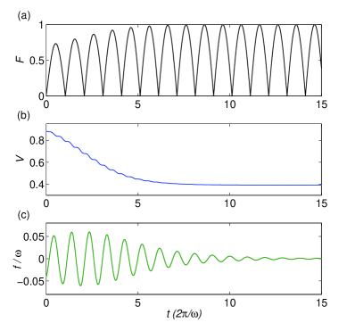
Figure 1: (Color online) Time evolution of (a) the fidelity $F$, (b) the Lyapunov function $V$ and (c) the control field $f(t)$ for the Hadamard gate. The operator $U$ is driven to $O_{H}$ with $F\approx 0.999$ at $t=9.62$. As the Lyapunov function decrease monotonically, fidelity larger than $0.999$ can be achieved at times later than $t=9.62$ . $K=0.05\omega$ and $\tau=1/\omega$ is chosen in this figure.

The Hamiltonian for a controlled single-qubit system can be expressed as

$$H=H_{0}+f(t)H_{1}$$ (16)

where $H_{0}=\frac{\omega}{2}\sigma_{z}$ is the free Hamiltonian and $H_{1}=\sigma_{x}$ represents the control Hamiltonian with $f(t)$ the control field. Within the time scale where decoherence is ignorable, the time-evolution operator $U$ is governed by

$$i\frac{dU}{dt}=(H_{0}+f(t)H_{1})U.$$ (17)

We now show how to realize the Hadamard gate $O_{H}$ by the Lyapunov control. According to our theory, we can choose the Lyapunov function as $V=1-\frac{1}{N^{2}}|\text{Tr}[\tilde{O}_{H}^{{\dagger}}(t)U]|^{2}$, where $N=2$ and $\tilde{O}_{H}(t)=e^{-iH_{0}t}O_{H}$. However, this Lyapunov function leads to $f(t)=0$ at the beginning of the control, an initial short non-zero control field is thus required to trigger the control. Alternatively, this problem can be solved by adopting $\tilde{O}^{{\dagger}}(t+\tau)$ instead of $\tilde{O}^{{\dagger}}(t)$ in the Lyapunov function as addressed in Section 2, i.e.,

$${V=1-\frac{1}{N^{2}}|\text{Tr}[\tilde{O}_{H}^{{\dagger}}(t+\tau)U]|^{2}}.$$ (18)

From this Lyapunov function the control field follows,

$$f(t)=K\Re\{\text{Tr}(-i\tilde{O}^{\dagger}_{H}(t\!+\!\tau)H_{1}U)[\text{Tr}(\tilde{O}^{\dagger}_{H}(t\!+\!\tau)U)]^{*}\}.$$ (19)

Numerical simulation results are shown in Fig.1, where we plot the fidelity between $U$ and $O_{H}$ (defined by Eq.(8)), the Lyapunov function and the control field as a function of time. The time-evolution operator $U$ reaches $O_{H}$ with fidelity $F\approx 0.999$ at $t=9.62$, see Fig.1 (a). Although the Lyapunov function does not decrease to $0$ as shown in Fig.1 (b), the time-evolution operator $U$ is driven to the orbit of $\tilde{O}_{H}(t+\tau)$, and then arrives at $O_{H}$ periodically with time. In this model, the Hadamard gate with high fidelity ($F\rightarrow 1$) can be achieved for any value of $K$ and $\tau$ in a finite time (except a $\tau$ that leads to $f(t)=0$).

Any single-qubit rotation can be expressed as $U_{R}=e^{-i\frac{\theta}{2}\vec{n}\cdot\vec{\sigma}}$ where $\theta$ is the rotation angle around the axis $\vec{n}=(\sin\omega\cos\phi,\sin\omega\sin\phi,\cos\omega)$ in the Bloch sphere. We further simulate our model with a large number of different target quantum gate $U_{R}$. For each $U_{R}$ , $\omega$ (from $0$ to $\pi$), $\theta$ (from $0$ to $2\pi$) and $\phi$ (from $0$ to $2\pi$) are randomly chosen. The results suggest that the proposed technique can produce any single-qubit rotations. The control mechanism of implementing a single-qubit gate $U=\left(\begin{array}[]{cc}a_{0}&a_{1}\\ b_{0}&b_{1}\\ \end{array}\right)$ with the free Hamiltonian $H_{0}=\sigma_{z}$ is interpreted as follows. First, the Lyapunov control (plus $H_{0}$) tips the basis state $|0\rangle$($|1\rangle$) to the latitude on the Bloch sphere where $\left[\begin{array}[]{cc}a_{0}(a_{1})\\ b_{0}(b_{1})\\ \end{array}\right]$ belongs. Then, free evolution (z-rotation) will drive the states to reach $\left[\begin{array}[]{cc}a_{0}(a_{1})\\ b_{0}(b_{1})\\ \end{array}\right]$ periodically.

3.2 Two-qubit gates

The controlled-NOT (CNOT) gate is widely used in quantum information processing, which flips the target qubit if and only if the controlled qubit is in state $|1\rangle$. It together with arbitrary single-qubit gates composes a set of universal quantum gates, namely, any operation possible on a quantum computer can be reduced as a finite sequence of gates from the universal gates [1]. The matrix representation for this gate in the bases $|00\rangle,|01\rangle,|10\rangle,|11\rangle$ is,

$$O_{C}=\left(\begin{array}[]{cccc}1&0&0&0\\ 0&1&0&0\\ 0&0&0&1\\ 0&0&1&0\\ \end{array}\right),$$ (24)

where the first qubit is the control qubit and the second is the target qubit.

Consider an NMR system with two spins coupled via Ising interaction, the Hamiltonian of such a system reads,

$$H_{0}=\frac{\omega_{1}}{2}\sigma_{z}^{(1)}+\frac{\omega_{2}}{2}\sigma_{z}^{(2)}+\frac{J}{4}\sigma_{z}^{(1)}\otimes\sigma_{z}^{(2)},$$ (25)

where $\omega_{1}$ and $\omega_{2}$ are the precession frequencies of the two spins and $J$ represents the coupling strength. We show that the CNOT gate can be realized by shinning a magnetic field on the second spin (qubit) via the control Hamiltonian,

$$H_{1}=\sigma_{x}^{(2)}.$$ (26)

The time-evolution operator $U$ satisfies,

$$i\frac{dU}{dt}=(H_{0}+f(t)H_{1})U.$$ (27)

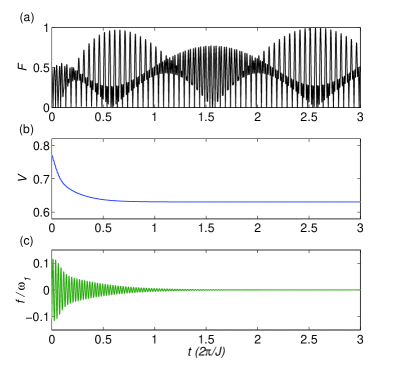
Figure 2: (Color online) The implementation of the CNOT gate with Ising coupling. The figure shows the (a) fidelity, (b) Lyapunov function and (c) control field versus time $t$. The time-evolution operator $U$ is driven to $O$ with $F\approx 0.9999$ at $t=2.56$ while the Lyapunov function decrease monotonically, although not convergent to 0. The parameters are, $\omega_{2}=2\omega_{1}$, $J=0.05\omega_{1}$, $K=0.1\omega_{1}$ and $\tau=0.3/\omega_{1}$

where the control field $f(t)$ can be realized by a time-dependent magnetic field. In this example, we still use $\tilde{O}(t+\tau)$ to define the Lyapunov function where different $\tau$ may lead to different fidelity. This is different from last example where a high fidelity (very close to 1) can be achieved for any $\tau$.

Now we go to the details. The Lyapunov function is defined as,

$$V=1-\frac{1}{N^{2}}|\text{Tr}(\tilde{O}^{{\dagger}}_{C}(t+\tau)U)|^{2},$$ (28)

where $\tilde{O}_{C}(t+\tau)=e^{-iH_{0}(t+\tau)}{O}_{C}$ and $N=4$. The control fields are given by,

$$f(t)=K\Re\{\text{Tr}(-i\tilde{O}^{\dagger}_{C}(t\!+\!\tau)H_{1}U)[\text{Tr}(\tilde{O}^{\dagger}_{C}(t\!+\!\tau)U)]^{*}\}.$$ (29)

We numerically simulate the model and plot the fidelity $F=\frac{|\text{Tr}(O_{C}^{{\dagger}}U)|}{4}$, the Lyapunov function $V$ and the control field $f(t)$ as as a function of time in Fig.2. We find that the fidelity reaches about $0.9999$ at $t=2.56$ as shown in Fig.2 (a). The parameter $\tau$ can be found numerically for a better performance. For example, we plot the evolution of fidelity with different $\tau$ in Fig.3. Such a figure shows appropriate $\tau$ as well as the time $t$ to achieve the CNOT gate. It is shown that the fidelity oscillates with $t$ which originates from the free Hamiltonian and can not be eliminated in the Schrodinger picture. Thus the gate time $t_{g}$ needs to be precisely chosen for high fidelity. Since $f(t)\rightarrow 0$ before $t_{g}$, in this sense, the fidelity is robust against the switching time of $f(t)$. For a given gate time $t$, the fidelity also depends on $\tau$ and may change dramatically at certain values of $\tau$ (we call these values $\tau^{\prime}$) as seen in Fig.3. However, when implementing a quantum gate, $\tau$ and $f(t)$ are known in advance by computer simulation. So the robustness against $\tau$ need not be considered in experiments. The reason for the sudden change of fidelity is that when $\tau=\tau^{\prime}$, the tracked operator $\tilde{O}_{C}(t+\tau^{\prime})$ is ineffective which leads to $f(0)=0$ and $f(t)\approx 0$ when $t$ is small. Then, $\tau_{1}=\tau^{\prime}+\varepsilon$ and $\tau_{2}=\tau^{\prime}-\varepsilon$ ($\varepsilon$ is infinitesimal) will generate significantly different control fields as well as fidelities although $\tau_{1}\approx\tau_{2}$. See that a typical $\tau^{\prime}$ is $0$.

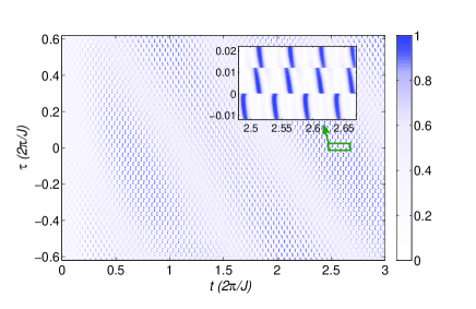
Figure 3: (Color online) Fidelity versus $t$ and $\tau$. The parameters chosen are the same as in Fig.2. The characteristic time scale of $\tilde{O}(t+\tau)$ is $1/\omega_{1}$ and $1/J$ ($1/J\geq 1/\omega_{1}$), thus the range of $\tau$ is chosen with a scale of $1/J$ and both positive and negative $\tau$ is considered. With the help of this figure, we can choose optimal $\tau$ and $t$ with both high fidelity and short time for implementing the CNOT gate.

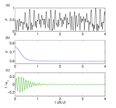
Figure 4: (Color online) The implementation of the CNOT gate with Heisenberg coupling. The figure shows (a) the fidelity, (b) the Lyapunov function and (c) the control field as a function of $t$. Parameters are set as $\omega_{2}=2\omega_{1}$, $J=0.2\omega_{1}$, $K=0.2\omega_{1}$ and $\tau=0.2/\omega_{1}$. Note that despite $\omega_{2}-\omega_{1}=5J$, and $\omega_{2}=2\omega_{1}=10J$, the Heisenberg interaction can not be approximated by the Ising interaction, this can be found by calculating the distance between the two time-evolution operators, corresponding to the two interaction, respectively.

The Ising coupling favors the implementation of the CNOT gate since the time-evolution operator governed by $H=J\sigma_{z}\otimes\sigma_{z}$ is equivalent to a CNOT gate up to one-qubit rotations [36]. In contrast, more operations are needed to realize the CNOT gate with the Heisenberg coupling [36]. Fortunately, the Heisenberg coupling may be reduced to the Ising coupling when the condition $|\omega_{1}-\omega_{2}|\gg J$ is satisfied [37, 38]. We now show that the CNOT gate can also be realized in a two-qubit system with Heisenberg coupling in a similar manner as in the case of Ising coupling.

Consider a two-qubit system with Heisenberg coupling, the free Hamiltonian takes,

$$H_{0}=\frac{1}{2}\omega_{1}\sigma_{z}^{(1)}+\frac{1}{2}\omega_{2}\sigma_{z}^{(2)}+\frac{1}{4}J\vec{\sigma}^{(1)}\cdot\vec{\sigma}^{(2)},$$ (30)

where $\vec{\sigma}^{(j)}=(\sigma_{x}^{(j)},\sigma_{y}^{(j)},\sigma_{z}^{(j)}),j=1,2$. With the same Lyapunov function Eq.(28), control Hamiltonian Eq.(26) and design of control field Eq.(29), we simulate the model and plot the fidelity , Lyapunov function and control field as a function of time in Fig.4. In this simulation, a stronger coupling constant $J$ is used such that the Heisenberg interaction can not be approximated by the Ising one. A fidelity about $0.994$ is obtained at $t=3.58$. Further numerical simulations show that for the Heisenberg Hamiltonian Eq.(30) with strong couplings, say $J\sim\omega_{i},i=1,2$, the implementation of the CNOT gate may have lower fidelity.

In this section, we use a single control field designed by the Lyapunov method to realize the CNOT gate in two-qubit quantum systems, different types of inter-qubit coupling are considered. It is worth noting that in these examples, the control is also effective if the control Hamiltonian Eq.(26) is replaced by $H_{1}=\sigma_{x}^{(1)}+\sigma_{x}^{(2)}$, this indicates that our proposal applies to homonuclear systems where two spins are coupled simultaneously to a single RF field, and the precession frequencies $\omega_{1}$ and $\omega_{2}$ in spins are replaced by the chemical shifts in the rotating frame [15]. This method can also be used to in NMR systems for other purposes to reduce the steps of operations. For example, in a homonuclear two-spin system with coupling, a shaped non-selective hard pulse acting on both spins can perform a local quantum gate on spin 1 while freezing spin 2 without refocusing technology [1, 37, 38].

4 Local equivalence operators

In the last section, we have shown that the Hadamard gate and the CNOT gate can be implemented by Lyapunov control. The fidelity reaches almost $100\%$ at specific times, but it would change after the gate time. In this section, we will show that by our method, the time-evolution operator for the models in Section 3.2 can be steered into a target class of operators (the local equivalence class of the CNOT gate) and stays in this class forever when the control fields are turned off.

Two two-qubit unitary operators $U_{1}$ and $U_{2}$ are called locally equivalent if they can be connected by local operations, i.e., $U_{1}=L_{1}U_{2}L_{2}$, where $L_{1},L_{2}\in SU(2)\otimes SU(2)$ are the combinations of single-qubit operations. Here we denote the local equivalence class of a unitary operator $O$ as $[O]$. Usually the realization of two-qubit gates are more costly (e.g., taking longer time, requiring more operations and so on) than that of single-qubit gates, hence a difficultly implemented two-qubit operation can be realized through its equivalent gate. On the other hand, any entangling two-qubit gate with single-qubit gates forms a universal set of quantum gates for quantum computing. Therefore, it is interesting to study how to realize the local equivalence gate for some particular two-qubit gates [21] such as the CNOT gate.

Makhlin proposed three local invariants [39] to characterize the non-local property of a two-qubit gate $U\in U(4)$, they are $d_{1}=\text{Re}G_{1},d_{2}=\text{Im}G_{1},$ and $d_{3}=G_{2}$, where $G_{1}=\text{Tr}^{2}m_{U}\det U^{{\dagger}}/16$ is complex and $G_{2}=(\text{Tr}^{2}m_{U}-\text{Tr}m_{U}^{2})\det{U^{{\dagger}}/4}$ is real. $m_{U}$ is defined as $m_{U}=Q^{T}U^{T}Q^{*}Q^{{\dagger}}UQ$ with

$$Q=\frac{1}{\sqrt{2}}\left(\begin{array}[]{cccc}1&0&0&i\\ 0&i&1&0\\ 0&i&-1&0\\ 1&0&0&-i\\ \end{array}\right).$$ (35)

Two two-qubit unitary gates are locally equivalent if they have the same $d_{i}$ $(i=1,2,3)$. In order to quantify the distance between a unitary operator $U$ and the equivalence set of the CNOT gate $[O_{C}]$, we define $D=\sqrt{(d_{1}-d^{\prime}_{1})^{2}+(d_{2}-d^{\prime}_{2})^{2}+(d_{3}-d^{\prime}_{3})^{2}}$ as a measure, where $d_{i}$ and $d^{\prime}_{i}$ are the invariants of $U$ and $O_{C}$, respectively.

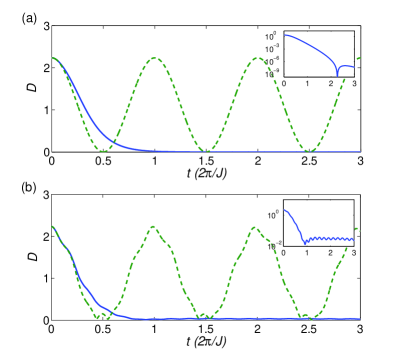
Figure 5: (Color online) Driving the time-evolution operator to local equivalence class of CNOT gate with (a) the Ising interaction and (b) the Heisenberg interaction. Blue solid lines represent time-dependence of $D$ under control (insets shows $D$ on a logarithmic scale). Green dashed lines correspond to $D$ without control ($f(t)=0$). The parameters used for (a) and (b) are the same as that in Fig. 2 and Fig.4, respectively.

For the Ising model Eq.(25), we find that once the time evolution operator is driven to the orbit of $\tilde{O}_{C}(t+\tau)$, it would stay in $[O_{C}]$ forever, even if the control fields are turned off. Now we show this point in detail. For the Ising model without control, the time-evolution operator in the orbit of $\tilde{O}_{C}(t+\tau)$ satisfies $U=e^{i\theta}e^{-iH_{0}t^{\prime}}O_{C}$, where $\theta$ and $t^{\prime}$ are real numbers. $U$ can be decomposed as $U=e^{i\theta}U_{a}U_{b}O_{C}$, where $U_{a}=e^{-i(\frac{\omega_{1}}{2}\sigma^{(1)}_{z}+\frac{\omega_{2}}{2}\sigma^{(2)}_{z})t^{\prime}}$ (local operation) and $U_{b}=e^{-i\frac{J}{4}\sigma^{(1)}_{z}\otimes\sigma^{(2)}_{z}t^{\prime}}$. If the distance $D$ between $M=e^{i\theta}U_{b}O_{C}$ and $O_{C}$ is zero, then $M$ and $O_{C}$ are locally equivalent. To calculate the distance, we need $m_{M}$ that takes,

$$m_{M}=Q^{T}M^{T}Q^{*}Q^{{\dagger}}MQ\quad\quad\quad\quad\quad$$

$$=e^{i2\theta}\!\left(\begin{array}[]{cccc}0\quad\ \ \ \sin(\frac{Jt^{\prime}}{2})\quad-\cos(\frac{Jt^{\prime}}{2})\quad\quad 0\\ \sin(\frac{Jt^{\prime}}{2})\quad\ \ \ \ 0\quad\quad 0\quad\ \ -\cos(\frac{Jt^{\prime}}{2})\\ -\cos(\frac{Jt^{\prime}}{2})\quad\ 0\quad\quad 0\quad\ \ -\sin(\frac{Jt^{\prime}}{2})\\ \ 0\quad-\cos(\frac{Jt^{\prime}}{2})\quad-\sin(\frac{Jt^{\prime}}{2})\quad\quad 0\\ \end{array}\right).$$ (40)

With the definition of local invariants, we have $d_{1}=\Re G_{1}=0,d_{2}=\Im G_{1}=0$ and $d_{3}=G_{2}=1.$ which are also the local invariants of $O_{C}$ regardless of $t^{\prime}$, $J$ and $\theta$. Therefore, $U$ and $O_{C}$ are locally equivalent. This fact can be exploited to create the CNOT gate at a more flexible time. Note that when the coupling $\sigma_{z}^{(1)}\sigma_{z}^{(2)}$ can not be switched off, the CNOT gate can be achieved only at specific times with the help of local operations [36]. However, if the evolution operator keeps in $[O_{C}]$, the CNOT gate can be obtained at any time with the help of local operations.

Next, we numerically simulate Eq.(27) with the same parameters ($\omega_{1,2},J,K$ and $\tau$ ) as in Fig.2 and calculate the distance between the time-evolution operator $U$ and $[O_{C}]$. The result is plotted with blue solid line in Fig.5 (a). We find that the time-evolution operator is driven to $[O_{C}]$ with high precision and stays in $[O_{C}]$ forever. Note that without the Lyapunov controls, the local invariants of $U(t)$ (obtained by setting $H_{1}=0$ in Eq.(27) with initial condition $U(0)=I$) evolve as $d_{1}=\cos^{2}(\frac{J}{2}t),d_{2}=0,d_{3}=2+\cos(Jt)$. The distance between $U(t)$ and $[O_{C}]$ is $D=\sqrt{5}\cos^{2}(\frac{J}{2}t)$, which reaches zero only when $t=(2n+1)\pi/J$ shown by the green-dashed line in Fig.5(a). Simulations with different $\omega_{1}$, $\omega_{2}$ and $J$ suggest that the time-evolution operator can be driven to $[O_{C}]$ for a wide range of parameters.

For the two-spin model with the Heisenberg interaction Eq.(30), the time-evolution operator $U=e^{i\theta}e^{-iH_{0}t^{\prime}}O_{C}$ can not stay in $[O_{C}]$. Nevertheless, it is still possible to drive the time-evolution operator approximately to $[O_{C}]$ when the two spins are weakly coupled and have a large difference at the precession frequency. To illustrate this, we simulate the Heisenberg model with the same parameters as in Fig.4 and plot the distance $D$ between $U$ and $[O_{C}]$ in Fig.5(b) (blue solid line). We find that the time-evolution operator can be driven to $[O_{C}]$, but the performance is not as perfect as that with the Ising interaction. Large difference at the precession frequencies and weaker coupling between the spins can improve the performance.

5 Summary

We present a Lyapunov control design to produce a quantum gate (or a class of quantum gates) in the Schrödinger picture. Considering that a unitary operator is usually not stationary under free evolution, a tracking strategy is adopted to steer the time-evolution operator to the orbit of target operator so as to reach the target. We introduce an adjustable parameter $\tau$ into the tracked operator such that the time-evolution operator can be easily driven to the target operator with high precision. We apply the proposal to the implementation of the Hadamard gate and the CNOT gate at some instance of time. Besides, we find that with the Ising interaction, the time-evolution operator can be driven into the local equivalence class of the CNOT gate and stay in that class forever. The advantages of the traditional Lyapunov control, e.g., easy and flexible design of control fields, no measurement induced decoherence, will contribute to the implementation of quantum gates. Meanwhile, there are some limitations to be improved in our method. First, the gate time $t_{g}$ is determined after the simulation which may be inconvenient when the control is applied. Second, our method may not be effective in general to implement other quantum gates or realize quantum gates in other (complex) Hamiltonian systems. At last, the fact that the evolution operator can be driven into the equivalence class of the CNOT gate may not be available with other coupling Hamiltonians.

6 Acknowledgements

This work is supported by the NSF of China under Grants Nos 61078011, 10935010 and 11175032.

7 References

References

- [1] M. A. Nielsen, I. L. Chuang, Quantum Computation and Quantum Information, Cambridge University Press, Cambridge, 2000.
- [2] J. Kofler, A. Zeilinger, European Review 18 (2010) 469.
- [3] P. O. Schmidt, T. Rosenband, C. Langer, W. M. Itano, J. C. Bergquist, D. J. Wineland, Science 309 (2005) 749.
- [4] C. F. Roos, M. Chwalla, K. Kim, M. Riebe, R. Blatt, Nature 443 (2006) 316.
- [5] D. D’Alessandro, Introduction to Quantum Control and Dynamics, Taylor and Francis Group, Boca Raton 2007.
- [6] D. Dong , I. R. Petersen, IET Control Theory Appl. 4 12 (2010) 2651.
- [7] A. Carlini, A. Hosoya, T. Koike, Y. Okudaira, Phys. Rev. Lett. 96 (2006) 060503.
- [8] J. P. Palao, R. Kosloff, Phys. Rev. Lett. 89 (2002) 18.
- [9] M. Lapert, J. Salomon, and D. Sugny, Phys. Rev. A 85 (2012) 033406.
- [10] S. G. Schirmer, A. D. Greentree, V. Ramakrishna, H. Rabitz, J. Phys. A: Math. Gen. 35 (2002) 8315.
- [11] D. Dong, I. R. Petersen, Automatica 48 (2012) 725.
- [12] H. M. Wiseman, G. J. Milburn, Phys. Rev. Lett. 70 (1993) 548.
- [13] F. Verstraete, M. M. Wolf, J. I. Cirac, Nat. Phys. 5 (2009) 633.
- [14] S. E. Sklarz, D. J. Tannor, Chem. Phys. 322 (2006) 87.
- [15] Z. Wu, J. Li, W. Zheng, J. Luo, M. Feng, X. Peng, Phys. Rev. A 84 (2011) 042312.
- [16] X. Wang, S. Vinjanampathy, F. W. Strauch, K. Jacobs, Phys. Rev. Lett. 107 (2012) 177204.
- [17] B. Rowland, J. A. Jones, Phil. Trans. R. Soc. A 370 (2012) 4636.
- [18] N. Khaneja, T. Reiss, C. Kehlet, T. Schulet-Herbrüggen, S. J. Glaser, J. Magn. Reson. 172 (2005) 296.
- [19] N. Khaneja, S. J. Glaser, R. Brockett, Phys. Rev. A 65 (2002) 032301.
- [20] P. de Fouquieres, Phys. Rev. Lett. 108 (2012) 110504.
- [21] M. M. Müller, D. M. Reich, M. Murphy, H. Yuan, J. Vala, K. B. Whaley, T. Calarco, C. P. Koch, Phys. Rev. A 84 (2011) 042315.
- [22] S. Grivopoulos, B. Bamieh, Proceedings of the 42nd IEEE Conference on Decision and Control, Maui, Hawaii (2003).
- [23] M. Mirrahimi, P. Rouchou, G. Turinici, Automatica 41 (2005) 1987.
- [24] S. Kuang, S. Cong, Automatica 44 (2008) 98.
- [25] X. Wang, S. G. Schirmer, IEEE Transactions on Automatic Control 55 (2010) 10.
- [26] W. Wang, L. C. Wang, X. X. Yi, Phys. Rev. A 82 (2007) 034308.
- [27] X. Wang, S. G. Schirmer, Phys. Rev. A 80 (2009) 042305.
- [28] W. Wang, S. C. Hou, X. X. Yi, Ann. Phys. 327 (2012) 1293.
- [29] S. C. Hou, M. A. Khan, X. X. Yi, D. Dong, I. R. Petersen, Phys. Rev. A 86 (2012) 022321.
- [30] J. Sharifi, H. Momeni, Phys. Lett. A 375 (2011) 522.
- [31] W. Yang, J. Sun, Phys. Lett. A 377 (2013) 851.
- [32] M. Sugawara, J. Chem. Phys. 118 (2003) 6784.
- [33] S. Ashhab, P. C. de Groot, F. Nori, Phys. Rev. A 85 (2012) 052327.
- [34] J. T. Thomas, M. Lababidi, M. Tian, Phys. Rev. A 84 (2011) 042335.
- [35] G. Wang, Phys. Rev. A 84 (2011) 052328.
- [36] N. Schuch, J. Siewert, Phys. Rev. A 67 (2003) 032301.
- [37] L. M. K. Vandersypen, I. L. Chuang, Rev. Mod. Phys. 76 (2004) 4.
- [38] Z. Zhang, G. Chen, Z. Diao, P. R. Hemmer, Advances in Mechanics and Mathematics 17 (2009) 465.
- [39] Y. Makhlin, Quantum Inf. Process. 1 (2002) 243.