Demixing and symmetry breaking in binary dipolar Bose-Einstein condensate solitons

Abstract

We demonstrate fully demixed (separated) robust and stable bright binary dipolar Bose-Einstein condensate soliton in a quasi-one-dimensional setting formed due to dipolar interactions for repulsive contact interactions. For large repulsive interspecies contact interaction the first species may spatially separate from the second species thus forming a demixed configuration, which can be spatially-symmetric or symmetry-broken. In the spatially-symmetric case, one of the the species occupies the central region, whereas the other species separates into two equal parts and stay predominantly out of this central region. In the symmetry-broken case, the two species stay side by side. Stability phase diagrams for the binary solitons are obtained. The results are illustrated with realistic values of parameters in the binary ¹⁶⁴Dy-¹⁶⁸Er and ¹⁶⁴Dy-¹⁶²Dy mixtures. The demixed solitons are really soliton molecules formed of two types of atoms. A proposal for creating dipolar solitons in experiments is also presented.

I Introduction

Quasi-one-dimensional (quasi-1D) bright soliton and soliton train were created and investigated experimentally in Bose-Einstein condensate (BEC) of ⁷Li 1 and ⁸⁵Rb atoms 3 . These quasi-1D solitons appear for attractive contact interaction in an axially-free BEC under radial harmonic trap 4 . However, due to collapse instability, in three dimensions (3D), such solitons are fragile and can accommodate only a small number of atoms.

Recent observation of BECs of ¹⁶⁴Dy ExpDy ; dy , ¹⁶⁸Er ExpEr and ⁵²Cr cr ; saddle atoms with large magnetic dipole moments has opened new directions of research in BEC solitons. In dipolar BECs, in addition to the quasi-1D solitons 1D ; 1Da , one could also have quasi-two-dimensional (quasi-2D) solitons 2D and vortex solitons ol2D . Moreover, dipolar BEC solitons can be stabilized when the harmonic trap(s) is (are) replaced by periodic optical-lattice trap(s) in quasi-1D ol1D and quasi-2D ol2D configurations. More interestingly, one can have dipolar BEC solitons for fully repulsive contact interaction 1D . Hence these solitons stabilized solely by long-range dipolar interaction are less vulnerable to collapse in 3D for a large number of atoms due to the repulsive contact interaction. This creates a new scenario for robust solitons of large number of atoms stabilized by short-range repulsion and long-range inter- and intraspecies dipolar attraction. One can study the interplay between the long-range anisotropic dipolar interactions and variable contact interactions using a Feshbach resonance fesh in a binary dipolar BEC soliton.

In a quasi-1D binary dipolar mixture mfb2 ; mfb3 free to move along the polarization $z$ direction, for large repulsive interspecies contact interaction, we demonstrate fully demixed (separated) bright dipolar binary solitons with a minimum of spatial overlap between the two species stabilized by long-range dipolar interactions for repulsive intraspecies contact interactions. The demixed binary soliton could be spatially symmetric while one of the species occupies the central region ($|z|<z_{0}$) and the other species stays symmetrically in both peripheral regions ($|z|>z_{0}$). For the same set of parameters (number of atoms and dipolar and contact interactions), the binary soliton could also stay in a stable but symmetry-broken spatially asymmetric shape where the two species lie side by side along the $z$ direction.

The demixed quasi-1D dipolar binary solitons are really soliton molecules. The binding between two (spatial-symmetry-broken) or three (spatially symmetric) solitons formed of two types of dipolar atoms is provided by the long-range interspecies dipolar interaction, which is attractive along the axial polarization direction. Previous consideration of dipolar soliton molecules was limited to two component solitons of the same species of atoms 1D .

We consider the numerical solution of a three-dimensional mean-field model mfb2 ; mfb3 of bright binary dipolar BEC solitons. We illustrate our findings using realistic values of inter- and intraspecies contact and dipolar interactions in the binary dipolar ¹⁶⁴Dy-¹⁶⁸Er and ¹⁶⁴Dy-¹⁶²Dy mixtures. The repulsive interspecies contact interaction plays a crucial role for the appearance of the demixed binary dipolar solitons. The domain of demixed solitons is illustrated in phase diagrams involving critical number of atoms and the interspecies scattering length. The profiles of the binary soliton are displayed in 3D isodensity plots of the two components. The stability of the solitons is demonstrated by considering a time evolution of the binary soliton when the inter- or intraspecies contact interaction is perturbed with a small time-dependent oscillating part. A steady propagation of the binary soliton under such a perturbation over a long period of time establishes the stability.

As these solitons are stable and robust, they can be created and studied in laboratory and we suggest a way of achieving this goal. First, a highly cigar-shaped dipolar BEC with appropriate number of atoms has to be created. Then the axial trap is to be removed slowly and linearly is a small interval of time while the axially trapped quasi-1D dipolar BEC will turn into an axially free quasi-1D dipolar BEC soliton. The viability of this procedure is demonstrated by real-time simulation of the mean-field model. As the dipolar soliton is an eigenstate of the mean-field model a very slow turn-off of the axial trap will always lead to a stable soliton. However, a reasonably quick turn-off is found to lead to a stable soliton as demonstrated in this paper. A nondipolar soliton is highly fragile and cannot be created in this fashion.

In Sec. II the time-dependent 3D mean-field model for the binary dipolar BEC soliton is presented. The results of numerical calculation are shown in Sec. III. The domain of a stable binary soliton is illustrated in stability phase diagrams showing the maximum number of atoms versus interspecies scattering length for fixed values of inter- and intraspecies dipolar interactions and intraspecies scattering lengths. The domain of mixed and demixed binary solitons are identified and the demixed solitons are further classified by spatially-symmetric and symmetry-broken types. The 3D isodensity profiles of the symmetric and symmetry-broken binary solitons are contrasted for the same set of parameters. The viability of preparing these solitons experimentally by relaxing the axial trap on a quasi-1D binary mixture is demonstrated by real-time simulation of the mean-field model. A similar demonstration for a single-component dipolar quasi-1D soliton was also made. Finally, in Sec. IV a brief summary of our findings is presented.

II Mean-field model for binary mixture

The extension of the mean-field Gross-Pitaevskii (GP) equation to a binary dipolar boson-boson mfb2 ; mfb3 and boson-fermion skabf mixtures are well established, and, for the sake of completeness, we make a brief summary of the same appropriate for this study. We consider a bright binary dipolar BEC soliton, with the mass, number of atoms, magnetic dipole moment, and scattering length for the two species $i=1,2,$ given by $m_{i},N_{i},\mu_{i},a_{i},$ respectively. The intra- ($V_{i}$) and interspecies ($V_{12}$) interactions for two atoms at $\bf r$ and $\bf r^{\prime}$ are

$$V_{i}({\bf R})=\frac{\mu_{0}\mu_{i}^{2}}{4\pi}\frac{1-3\cos^{2}\theta}{|{\bf R}|^{3}}+\frac{4\pi\hbar^{2}a_{i}}{m_{i}}\delta({\bf R}),$$ (1)

$$V_{12}({\bf R})=\frac{\mu_{0}\mu_{1}\mu_{2}}{4\pi}\frac{1-3\cos^{2}\theta}{|{\bf R}|^{3}}+\frac{2\pi\hbar^{2}a_{12}}{m_{R}}\delta({\bf R}),$$ (2)

respectively, where $a_{12}$ is the intraspecies scattering length, $\mu_{0}$ is the permeability of free space, $\theta$ is the angle made by the vector ${\bf R}$ with the polarization $z$ direction, $\bf R=r-r^{\prime},$ and $m_{R}=m_{1}m_{2}/(m_{1}+m_{2})$ is the reduced mass. With these interactions, the coupled GP equations for the binary dipolar BEC can be written as mfb ; mfb2 ; mfb3

$$\,{\mbox{i}}\hbar\frac{\partial\phi_{1}({\bf r},t)}{\partial t}={\Big{[}}-\frac{\hbar^{2}}{2m_{1}}\nabla^{2}+\frac{1}{2}m_{1}\omega_{1}^{2}\rho^{2}$$

$$+\frac{4\pi\hbar^{2}}{m_{1}}{a}_{1}N_{1}|\phi_{1}({\bf r},t)|^{2}+\frac{2\pi\hbar^{2}}{m_{R}}{a}_{12}N_{2}|\phi_{2}({\bf r},t)|^{2}$$

$$+N_{1}\frac{\mu_{0}\ {\mu}^{2}_{1}}{4\pi}\int V_{\mathrm{dd}}({\mathbf{R}})|\phi_{1}({\mathbf{r}^{\prime}},t)|^{2}d{\mathbf{r}}^{\prime}$$

$$+N_{2}\frac{\mu_{0}\ {\mu}_{1}\mu_{2}}{4\pi}\int V_{\mathrm{dd}}({\mathbf{R}})|\phi_{2}({\mathbf{r}^{\prime}},t)|^{2}d{\mathbf{r}}^{\prime}{\Big{]}}\phi_{1}({\bf r},t),$$ (3)

$${\mbox{i}}\hbar\frac{\partial\phi_{2}({\bf r},t)}{\partial t}={\Big{[}}-\frac{\hbar^{2}}{2m_{2}}\nabla^{2}+\frac{1}{2}m_{2}\omega_{2}^{2}\rho^{2}$$

$$+\frac{4\pi\hbar^{2}}{m_{2}}{a}_{2}N_{2}|\phi_{2}({\bf r},t)|^{2}+\frac{2\pi\hbar^{2}}{m_{R}}{a}_{12}N_{1}|\phi_{1}({\bf r},t)|^{2}$$

$$+N_{2}\frac{\mu_{0}\ {\mu}^{2}_{2}}{4\pi}\int V_{\mathrm{dd}}({\mathbf{R}})|\phi_{2}({\mathbf{r}^{\prime}},t)|^{2}d{\mathbf{r}}^{\prime}$$

$$+N_{1}\frac{\mu_{0}\ {\mu}_{1}\mu_{2}}{4\pi}\int V_{\mathrm{dd}}({\mathbf{R}})|\phi_{1}({\mathbf{r}^{\prime}},t)|^{2}d{\mathbf{r}}^{\prime}\Big{]}\phi_{2}({\bf r},t),$$ (4)

$$V_{\mathrm{dd}}({\mathbf{R}})=\frac{1-3\cos^{2}\theta}{{\mathbf{R}}^{3}},\quad\rho^{2}=x^{2}+y^{2},\quad{\mbox{i}}=\sqrt{-1},$$ (5)

with normalization $\int d{\bf r}|\phi_{i}({\bf r},t)|^{2}=1$. Here $\omega_{i}$ are the angular frequencies of the traps acting on the two species in the transverse $\rho$ direction. The binary soliton is free to move in the axial $z$ direction.

The intra- and interspecies dipolar interactions are usually expressed in terms of the dipolar lengths $a_{\mathrm{dd}}^{(i)}$ and $a_{\mathrm{dd}}^{(12)}$, defined by

$$a_{\mathrm{dd}}^{(i)}=\frac{\mu_{0}\mu_{i}^{2}m_{i}}{12\pi\hbar^{2}},\quad a_{\mathrm{dd}}^{(12)}=\frac{\mu_{0}\mu_{1}\mu_{2}m_{R}}{6\pi\hbar^{2}}.$$ (6)

We express the strengths of the dipolar interactions by these lengths and transform Eqs. (3) and (II) into the following dimensionless form mfb2

$$\,{\mbox{i}}\frac{\partial\phi_{1}({\bf r},t)}{\partial t}={\Big{[}}-\frac{\nabla^{2}}{2}+\frac{1}{2}\rho^{2}$$

$$\,+g_{1}|\phi_{1}|^{2}+g_{12}|\phi_{2}|^{2}+g_{\mathrm{dd}}^{(1)}\int V_{\mathrm{dd}}({\mathbf{R}})|\phi_{1}({\mathbf{r}^{\prime}},t)|^{2}d{\mathbf{r}}^{\prime}$$

$$\,+g_{\mathrm{dd}}^{(12)}\int V_{\mathrm{dd}}({\mathbf{R}})|\phi_{2}({\mathbf{r}^{\prime}},t)|^{2}d{\mathbf{r}}^{\prime}{\Big{]}}\phi_{1}({\bf r},t),$$ (7)

$$\,{\mbox{i}}\frac{\partial\phi_{2}({\bf r},t)}{\partial t}={\Big{[}}-m_{12}\frac{\nabla^{2}}{2}+\frac{1}{2}m_{\omega}\rho^{2}$$

$$\,+g_{2}|\phi_{2}|^{2}+g_{21}|\phi_{1}|^{2}+g_{\mathrm{dd}}^{(2)}\int V_{\mathrm{dd}}({\mathbf{R}})|\phi_{2}({\mathbf{r}^{\prime}},t)|^{2}d{\mathbf{r}}^{\prime}$$

$$\,+g_{\mathrm{dd}}^{(21)}\int V_{\mathrm{dd}}({\mathbf{R}})|\phi_{1}({\mathbf{r}^{\prime}},t)|^{2}d{\mathbf{r}}^{\prime}{\Big{]}}\phi_{2}({\bf r},t),$$ (8)

where $m_{\omega}=\omega_{2}^{2}/(m_{12}\omega_{1}^{2}),$ $m_{12}={m_{1}}/{m_{2}},$ $g_{1}=4\pi a_{1}N_{1},$ $g_{2}=4\pi a_{2}N_{2}m_{12},$ $g_{12}={2\pi m_{1}}a_{12}N_{2}/m_{R},$ $g_{21}={2\pi m_{1}}a_{12}N_{1}/m_{R},$ $g_{\mathrm{dd}}^{(2)}=3N_{2}a_{\mathrm{dd}}^{(2)}m_{12},$ $g_{\mathrm{dd}}^{(1)}=3N_{1}a_{\mathrm{dd}}^{(1)},$ $g_{\mathrm{dd}}^{(12)}=3N_{2}a_{\mathrm{dd}}^{(12)}m_{1}/(2m_{R}),$ $g_{\mathrm{dd}}^{(21)}=3N_{1}a_{\mathrm{dd}}^{(12)}m_{1}/(2m_{R}).$ In Eqs. (7) and (8), length is expressed in units of oscillator length $l_{0}=\sqrt{\hbar/(m_{1}\omega_{1})}$, energy in units of oscillator energy $\hbar\omega_{1}$, probability density $|\phi_{i}|^{2}$ in units of $l_{0}^{-3}$, and time in units of $t_{0}=1/\omega_{1}$.

The dimensionless GP equation for a single-component dipolar quasi-1D soliton is 1D

$$\,{\mbox{i}}\frac{\partial\phi({\bf r},t)}{\partial t}={\Big{[}}-\frac{\nabla^{2}}{2}+\frac{1}{2}\rho^{2}+4\pi aN|\phi({\mathbf{r}},t)|^{2}$$

$$\,+3a_{\mathrm{dd}}N\int V_{\mathrm{dd}}({\mathbf{R}})|\phi({\mathbf{r}^{\prime}},t)|^{2}d{\mathbf{r}}^{\prime}{\Big{]}}\phi({\bf r},t),$$ (9)

where $N$ is the number of atoms, $a$ is the scattering length, $a_{\mathrm{dd}}$ the dipolar length.

III Numerical Results

We demonstrate stable demixed spatially-symmetric and asymmetric binary dipolar solitons for realistic values of atom numbers and interaction parameters in the ¹⁶⁴Dy-¹⁶⁸Er and ¹⁶⁴Dy-¹⁶²Dy mixtures. The ¹⁶⁴Dy and ¹⁶⁸Er atoms have the largest magnetic moments of all the dipolar atoms used in BEC experiments. For the ¹⁶⁴Dy-¹⁶⁸Er mixture, the ¹⁶⁴Dy atoms are labeled $i=1$ and the ¹⁶⁸Er atoms are labeled $i=2$. The magnetic moment of a ¹⁶⁴Dy atom is $\mu_{1}=10\mu_{B}$ ExpDy and of a ¹⁶⁸Er atom is $\mu_{2}=7\mu_{B}$ ExpEr with $\mu_{B}$ the Bohr magneton leading to the dipolar lengths $a_{\mathrm{dd}}^{(1)}\equiv\mu_{0}\mu_{1}^{2}m_{1}/(12\pi\hbar^{2})\approx 132.7a_{0}$, $a_{\mathrm{dd}}^{(2)}\equiv\mu_{0}\mu_{2}^{2}m_{2}/(12\pi\hbar^{2})\approx 66.6a_{0}$, and $a_{\mathrm{dd}}^{(12)}\equiv\mu_{0}\mu_{1}\mu_{2}m_{R}/(6\pi\hbar^{2})\approx 94.0a_{0}$, with $a_{0}$ the Bohr radius. For the ¹⁶⁴Dy-¹⁶²Dy mixture, the ¹⁶⁴Dy atoms are labeled $i=1$ and the ¹⁶²Dy atoms are labeled $i=2$. The magmetic moment of a ¹⁶²Dy atom is $\mu_{2}=10\mu_{B}$. Consequently the dipolar lengths are: $a_{\mathrm{dd}}^{(1)}\approx 132.7a_{0}$, $a_{\mathrm{dd}}^{(2)}\approx 131.0a_{0}$, and $a_{\mathrm{dd}}^{(12)}\approx 131.9a_{0}$. The fundamental constants used in the evaluation of these dipolar lengths are: $\mu_{B}=9.27401\times 10^{-24}$ Am², $a_{0}=5.292\times 10^{-11}$ m, $\mu_{0}=4\pi\times 10^{-7}$ N/A${}^{2},$ $\hbar=1.05457\times 10^{-34}$ m²kg/s, 1 amu = $1.66054\times 10^{-27}$ kg. The dipolar interaction in ¹⁶⁴Dy atoms is roughly double of that in ¹⁶⁸Er atoms and about eight times larger than that in ⁵²Cr atoms with a dipolar length $a_{\mathrm{dd}}\approx 15a_{0}$ cr . We consider the trap frequencies $\omega_{1}=\omega_{2}=2\pi\times 61.6$ Hz, so that the length scale $l_{0}\equiv\sqrt{\hbar/m_{1}\omega_{1}}\approx 1$ $\mu$m, and time scale $t_{0}\equiv\omega_{1}^{-1}\approx 2.6$ ms.

To the best of our knowledge the experimental values of none of the scattering lengths considered in this paper are known, except for the intraspecies scattering length of ¹⁶⁸Er atoms, where preliminary cross-dimensional thermalization measurements point to a scattering length between $150a_{0}$ and $200a_{0}$ ExpEr . Nevertheless, scattering lengths can be adjusted experimentally using a Feshbach resonance fesh .

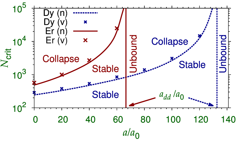
Figure 1: (Color online) Stability phase diagram illustrating the critical number of atoms in a single-component quasi-1D dipolar BEC soliton of ¹⁶⁴Dy or ¹⁶⁸Er atoms from numerical calculation (n) and variational approximation (v). The system is repulsive and unbound for $a\gtrsim a_{\mathrm{dd}}$. Stable quasi-1D solitons appear for $a\lesssim a_{\mathrm{dd}}$ and the number of atoms $N$ below a critical number $N_{\mathrm{crit}}$. The oscillator length $l_{0}=1$ $\mu$m.

We solve the 3D Eqs. (7) and (8) by the split-step Crank-Nicolson discretization scheme using both real- and imaginary-time propagation in 3D Cartesian coordinates independent of the underlying trap symmetry using a space step of 0.1 $\sim$ 0.2 and a time step of 0.001 $\sim$ 0.005 CPC . The dipolar potential term is treated by Fourier transformation in momentum space using a convolution theorem in usual fashion Santos01 .

We study demixing in binary solitons supported by long-range dipolar interactions for repulsive interspecies and intraspecies contact interactions. The repulsive contact interactions make the dipolar solitons less vulnerable to collapse for a larger number of atoms compared to the nondipolar solitons. However, to have a net attraction in the system, atoms with large magnetic dipole moments, such as ¹⁶⁴Dy and ¹⁶⁸Er are considered. In the quasi-1D shape, with radial harmonic trap, the dipolar interaction is attractive in the axial $z$ direction. The net repulsion in the transverse direction is balanced by the external harmonic trap.

III.1 Single component ¹⁶⁴Dy and ¹⁶⁸Er solitons

To have a feeling about the maximum number of atoms in a single-component quasi-1D dipolar soliton, first we solve Eq. (9) for different values of the scattering length $a$. We find that for interaction parameters of ¹⁶⁴Dy and ¹⁶⁸Er atoms the solitons are stable up to a critical maximum number of atoms, beyond which the system collapses. In Fig. 1 we plot this critical number $N_{\mathrm{crit}}$ versus $a$ from numerical simulation using Eq. (9) and from a Gaussian variational approximation to it as developed in Ref. 1D . The variational approximation leads to overbinding and hence can accommodate a larger number of atoms in a stable soliton as can be seen in Fig. 1. We find that a stable soliton is possible for $a\lesssim a_{\mathrm{dd}}$ and for a number of atoms below this critical number. The critical number of atoms increases with the increase of contact repulsion as $a\to a_{\mathrm{dd}}$, which is counterintuitive. The solitons are bound by long-range dipolar interaction and increase of contact repulsion gives more stability against collapse for a fixed dipolar interaction strength. In this phase diagram three regions are shown: stable, collapse and unbound. In the unbound region ($a\gtrsim a_{\mathrm{dd}}$) contact repulsion dominates over dipolar attraction and the soliton cannot be bound. In the collapse region, the opposite happens and the soliton collapses due to excess of attractive dipolar interaction along the axial $z$ direction. In the stable region there is a balance between attraction and repulsion and a stable soliton can be formed. So in our study of binary solitons we shall take $a\lesssim a_{\mathrm{dd}}.$ In this fashion, a binary soliton of large number of atoms could be created and this would be of greater experimental interest. In this study we take for the ¹⁶⁴Dy atoms $a_{1}=120a_{0}$, and for the ¹⁶⁸Er atoms $a_{2}=60a_{0}$. From Fig. 1 we see that for these values of scattering length a stable bright soliton can accommodate a large number of atoms of the two species.

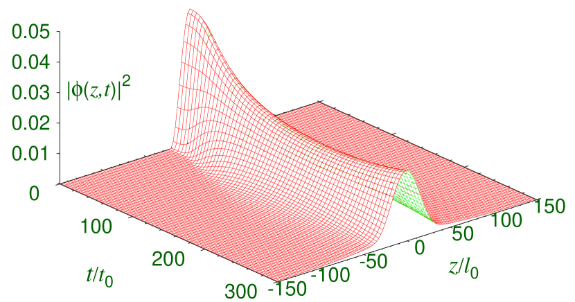
Figure 2: (Color online) Integrated 1D density $|\phi(z,t)|^{2}=\int dx\int dy|\phi({\bf r},t)|^{2}$ of ¹⁶⁴Dy atoms during real-time propagation when the axial trap of angular frequency $\omega=2\pi\times 2$ Hz on a quasi-1D dipolar BEC of 8000 ¹⁶⁴Dy atoms is removed linearly for $20>t/t_{0}>0$ and the resultant axially-free soliton is propagated. Parameters used in simulation: $a_{\mathrm{dd}}=132.7a_{0},a=120a_{0},\omega_{\rho}=2\pi\times 61$ Hz, $l_{0}=1$ $\mu$m.

As the dipolar solitons are stable and robust, it is relatively easy to make these solitons of a large number of atoms. The nondipolar solitons are usually tiny and fragile containing a small number of atoms 1 ; 3 . We illustrate a method for creating a dipolar soliton of 8000 ¹⁶⁴Dy atoms by real-time simulation of the GP equation (9) with the scattering length $a=120a_{0}$. By imaginary-time propagation we create a bound quasi-1D BEC in the trap $V({\bf r})=(\rho^{2}+\lambda^{2}z^{2})/2$ with $\lambda=0.03$. This corresponds to taking a weak axial trap along $z$ axis of angular frequency $\omega_{z}\approx 2\pi\times 2$ Hz compared to the strong radial trap in the $x-y$ plane of angular frequency $\omega_{\rho}=2\pi\times 61$ Hz. The 3D profile of the BEC as obtained in imaginary-time propagation is used as the initial state in the real-time routine. During real-time propagation, from $t/t_{0}=0$ to 20 the axial trap $\lambda^{2}z^{2}/2$ is gradually (linearly) reduced to zero, so that for $t/t_{0}>20$ the axially free quasi-1D soliton condition is realized. We continue the real-time propagation for $t/t_{0}>20$ for a reasonably large interval of time. Long sustained propagation of the central peak establishes the soliton nature of the axially-free dipolar BEC. The result of this simulation is presented in Fig. 2, where we show the integrated 1D density $|\phi(z,t)|^{2}=\int dx\int dy|\phi({\bf r},t)|^{2}$ during real-time propagation. Upon the relaxation of the axial trap reasonably quickly the soliton expands a little in the beginning before attaining the final shape, as can be seen in Fig. 2. We note that the solitonic nature of the axially free dipolar BEC is evident in Fig. 2. This approach can be used in a laboratory to create dipolar solitons. Fragile nondipolar solitons supported by contact attraction only cannot be easily prepared in this fashion.

III.2 Binary ¹⁶⁴Dy-¹⁶⁸Er soliton

Scattering lengths play important roles in the preparation of binary solitons and can be experimentally controlled independently by magnetic fesh and optical opfesh Feshbach resonance techniques. For ¹⁶⁴Dy atoms we take $a_{1}=120a_{0}$, and for ¹⁶⁸Er atoms we take $a_{2}=60a_{0}$. However, the interspecies scattering length $a_{12}$ plays a crucial role in demixing in binary solitons and will be considered as a variable. After some experimentation in numerical simulation we realized that a reasonably large interspecies scattering length $a_{12}$ ($\gtrsim 70a_{0}$) and the number of atoms of the species below a critical value is needed for the creation of a demixed binary dipolar soliton. For much larger values of the interspecies scattering length ($a_{12}\gtrsim 120a_{0}$), the repulsion could be sufficiently strong, so that solitons of the two species could not be bound to form a stable binary dipolar soliton. For larger values of the number of atoms, the system collapses due to a strong net dipolar interaction even for repulsive intraspecies interaction. The demixing takes place due to interspecies contact repulsion. For smaller values of interspecies scattering length, the repulsion is not sufficient for demixing and a mixed or overlapping configuration of binary dipolar BEC soliton is realized mfb3 .

A spatially-symmetric binary soliton is obtained by solving Eqs. (7) and (8) with imaginary-time propagation with the following spatially-symmetric Gaussian input for both the functions $\phi_{i}$:

$$\phi_{i}({\bf r})=\frac{\pi^{-3/4}}{w_{\rho}\sqrt{w}_{z}}\exp\left[-\frac{\rho^{2}}{2w_{\rho}^{2}}-\frac{z^{2}}{2w_{z}^{2}}\right],$$ (10)

where $w$’s are the respective widths. An initial guess of widths close to their final converged values facilitates convergence. The input (10) and the final binary soliton are spatially-symmetric around $z=0$. To obtain a symmetry-broken binary soliton, a symmetry-broken initial input is needed.

Now we display the typical profile of a spatially-symmetric demixed binary dipolar BEC soliton in Fig. 3 for 2000 ¹⁶⁴Dy atoms and 5000 ¹⁶⁸Er atoms for the interspecies scattering length $a_{12}=a($Dy-Er$)=90a_{0}$ and for large intraspecies scattering lengths: $a_{1}=a$(Dy) $=120a_{0}$, $a_{2}=a$(Er) = 60$a_{0}$. The species containing the larger number of atoms (¹⁶⁸Er) stay at the center and the species containing the smaller number of atoms (¹⁶⁴Dy) breaks into two equal parts, leave the central region occupied by ¹⁶⁸Er atoms and stays symmetrically on two sides of the ¹⁶⁸Er soliton with a minimum of interspecies overlap. Note that the “3D densities” plotted in this paper are the norms of the respective wave functions $|\phi_{i}|^{2}$, whereas the atom densities are $N_{i}|\phi_{i}|^{2}$.

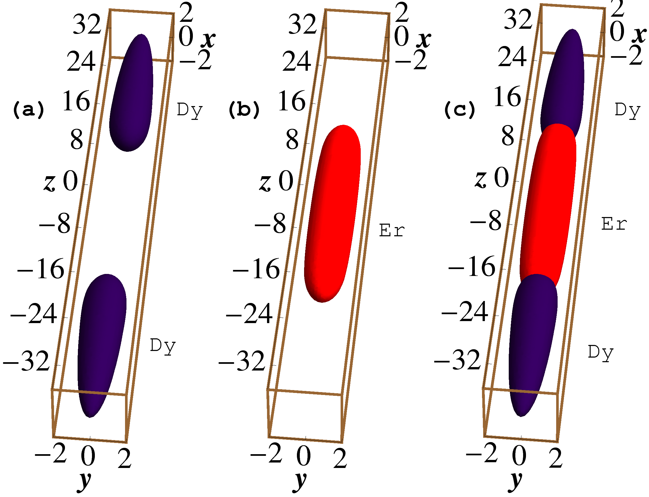
Figure 3: (Color online) 3D isodensity contour (a) $|\phi_{1}|^{2}$ of ¹⁶⁴Dy, (b) $|\phi_{2}|^{2}$ of ¹⁶⁸Er, and (c) $(|\phi_{1}|^{2}+|\phi_{2}|^{2})$ of the ¹⁶⁴Dy-¹⁶⁸Er mixture for the binary soliton of 2000 ¹⁶⁴Dy and 5000 ¹⁶⁸Er atoms with $a($Dy$)=120a_{0},a($Er$)=60a_{0},a($Dy-Er$)=90a_{0}$. The dimensionless lengths $x,y,$ and $z$ are in units of $l_{0}(\equiv 1$ $\mu$m). The density on contour is 0.002.

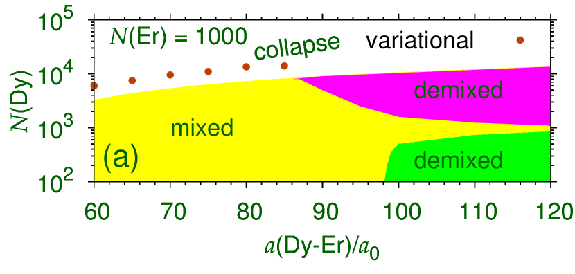
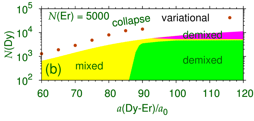
Figure 4: (Color online) Stability phase diagram for a binary ¹⁶⁴Dy-¹⁶⁸Er soliton for $N$(Er) = (a) 1000 and (b) 5000 atoms. The variational mixed-collapse border is shown by solid circles. The oscillator length $l_{0}=1$ $\mu$m, $a$(Dy)$=120a_{0},a$(Er)$=60a_{0}.$ Stable demixed binary soliton is observed in the darker (pink and green) region to the right while stable mixed binary soliton appears in the lighter (yellow) region to the left. For a spatially-symmetric demixed binary soliton, in the upper darker (pink) region the ¹⁶⁸Er atoms stay out and in the lower darker (green) region the ¹⁶⁴Dy atoms stay out of the central region ($z=0$).

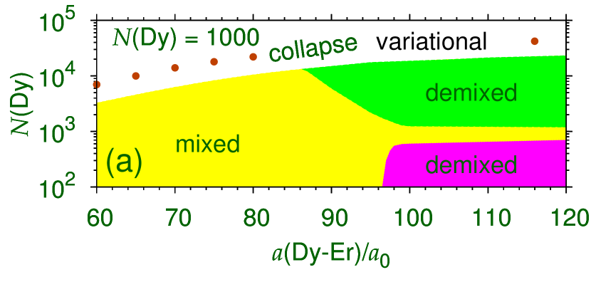
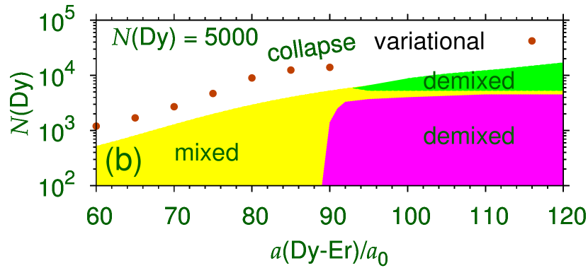
Figure 5: (Color online) Same as in Fig. 4 for (a) $N$(Dy) = 1000 and (b) 5000 atoms.

Next we show the stability phase diagrams for the appearance of the demixed binary dipolar soliton in the ¹⁶⁴Dy-¹⁶⁸Er mixture for different number of atoms and variable interspecies scattering length $a_{12}$. In Figs. 4 (a) and (b) we show the critical number of ¹⁶⁴Dy atoms $N_{1}=N$(Dy) versus $a_{12}$ for the numbers of ¹⁶⁸Er atoms $N_{2}=N$(Er) $=1000,5000$, respectively. The binary system collapses for $N$(Dy) larger than these critical values. For small values of $a_{12}$ the binary soliton is mixed and it gets demixed for large values of $a_{12}$ due to strong interspecies contact repulsion. A Gaussian variational approximation to Eqs. (7) and (8) was developed in Ref. mfb3 for a mixed binary soliton. This approximation using a mixed configuration of the two solitons can be used to calculate the mixed-collapse boundary. The variational results for this boundary are also shown in Figs. 4. As the variational approximation overbinds the binary soliton, it shows a larger stable region than the full numerical solution. For $a_{12}\lesssim 80a_{0}$ the binary solitons are spatially-symmetric and mixed and the two species of atoms lie on top of each other. However, for larger $a_{12}$ the contact repulsion between the two species of atoms increases and the system gets demixed. There are two ways this demixing takes place. The demixed binary soliton can either be spatially-symmetric around $z=0$, or it can be spatially asymmetric around $z=0$. The two configurations are possible for identical parameters of the binary system, e.g., number of atoms of the two components, and all dipolar and contact interaction strengths. However, there is a region around $N_{1}\approx N_{2}$ for these larger values of $a_{12}$, where the solitons continue in a mixed configuration. On both sides of this region demixing can take place. In the spatially-symmetric configuration, one of the components (the one containing the larger number of atoms) continues in the spatially-symmetric state at $z=0.$ The other component (the one containing the smaller number of atoms) divides into two equal pieces, separates from each other, leaves the central region occupied by the first component around $z=0$, moves in opposite directions and stays for $|z|>z_{0}$ in a spatially-symmetric configuration as shown in Fig. 3. In the spatial-symmetry-broken configuration, both components remain as single pieces and move away from each other and eventually lie on both sides of $z=0$ in a spatially-asymmetric configuration. In Figs. 5 (a) and (b) we show the critical number of ¹⁶⁸Er atoms $N_{2}=N$(Er) versus $a_{12}$ for the numbers of ¹⁶⁴Dy atoms $N_{1}=N$(Dy) $=1000,5000$, respectively. A similar scenario emerges in Figs. 5 as in Figs. 4.

In Fig. 3 we presented a spatially-symmetric demixed binary dipolar soliton with 2000 ¹⁶⁴Dy and 5000 ¹⁶⁸Er atoms. In this case, ¹⁶⁸Er atoms lie in the central region whereas ¹⁶⁴Dy atoms move away from the central region. The situation changes with a larger number of ¹⁶⁴Dy atoms. This is illustrated Fig. 6 with 5000 ¹⁶⁴Dy atoms and 1000 ¹⁶⁸Er atoms. In this case, in the isodensity contour of the binary soliton the roles of ¹⁶⁴Dy and ¹⁶⁸Er atoms are changed compared to that in Fig. 3. Now, contrary to that in Fig. 3, the ¹⁶⁴Dy atoms occupy the central region and the ¹⁶⁸Er atoms occupy the peripheral region. In Figs. 4 and 5 in the darker pink region in the spatially-symmetric configuration the ¹⁶⁴Dy atoms stay at the center and ¹⁶⁸Er atoms stay in the outer region and the opposite happens in the darker green region. The binary soliton of Fig. 3 lies in the darker green area of Fig. 4 (b), and the binary soliton of Fig. 6 lies in the darker pink area of Fig. 5 (b).

Figure 6: (Color online) 3D isodensity contour (a) $|\phi_{2}|^{2}$ of ¹⁶⁸Er, (b) $|\phi_{1}|^{2}$ of ¹⁶⁴Dy, and (c) $(|\phi_{1}|^{2}+|\phi_{2}|^{2})$ of the ¹⁶⁴Dy-¹⁶⁸Er mixture for the binary soliton of 5000 ¹⁶⁴Dy and 1000 ¹⁶⁸Er atoms with $a($Dy$)=120a_{0},a($Er$)=60a_{0},a($Dy-Er$)=90a_{0}$. The dimensionless lengths $x,y,$ and $z$ are in units of $l_{0}(\equiv 1$ $\mu$m). The density on contour is 0.002.

It is important to establish the stability of these spatially-symmetric solitons under small variation of the parameters of the initial state. To achieve this, we consider the final state of the spatially-symmetric binary soliton as obtained from the imaginary-time routine and use it as the initial state in the real-time program. First, we perform the numerical simulation with the binary soliton of Fig. 3 with the time-dependent interspecies scattering length $a_{12}=90a_{0}+10a_{0}\cos(t/t_{0})$, while the initial state was obtained with $a_{12}=90a_{0}$. All other contact and dipolar interaction strengths are maintained at their initial values. This perturbation should be sufficient to destroy an unstable soliton. The system executes small oscillation around the stable position. Otherwise, no noticeable change is observed after 100 units of real-time propagation. Our results are illustrated in Figs. 7 and 8. In Fig. 7 we illustrate the contour plot of integrated 1D density $|\phi_{i}(z,t)|^{2}=\int\int dxdy|\phi(x,y,z,t)|^{2}$ during real-time propagation. The visual profile of the solitons in Fig. 7 maintain a constant width and do not show a sign of instability. To have a more quantitative view, in Fig. 8 we plot the initial and final 1D densities $|\phi_{i}(z,t)|^{2}$ at times $t/t_{0}=0$ and 100 during real-time propagation. This clearly demonstrates the stability of the binary dipolar soliton under small oscillation.

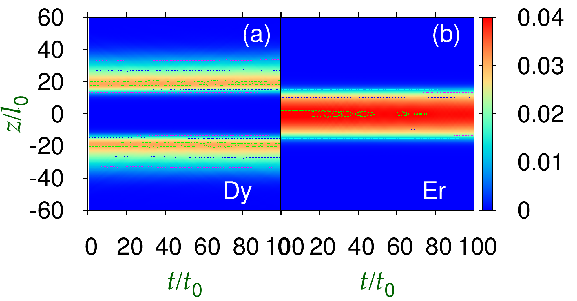
Figure 7: (Color online) Contour plot of integrated 1D densities $|\phi_{i}(z,t)|^{2}=\int dx\int dy|\phi({\bf r},t)|^{2}$ of ¹⁶⁴Dy and ¹⁶⁸Er atoms when the binary soliton of Fig. 3 is propagated with the time-dependent interspecies scattering length $a($Dy-Er$)=90a_{0}+10a_{0}\cos(t/t_{0})$ with all other parameters maintained at their time-independent initial values.

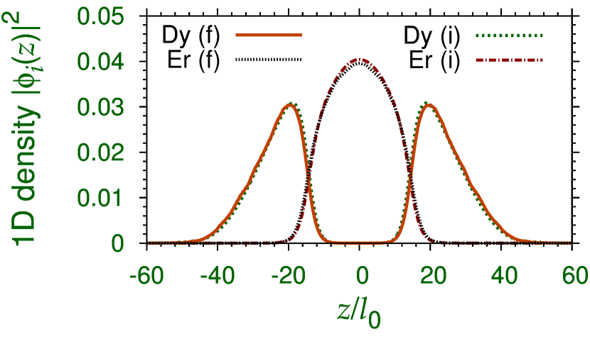
Figure 8: (Color online) Initial (i) at $t=0$ and final (f) at $t=100$ values of integrated 1D densities $|\phi_{i}(z)|^{2}=\int dx\int dy|\phi({\bf r})|^{2}$ of ¹⁶⁴Dy and ¹⁶⁸Er atoms in the binary ¹⁶⁴Dy-¹⁶⁸Er soliton of Fig. 3 during real-time propagation of Fig. 7.

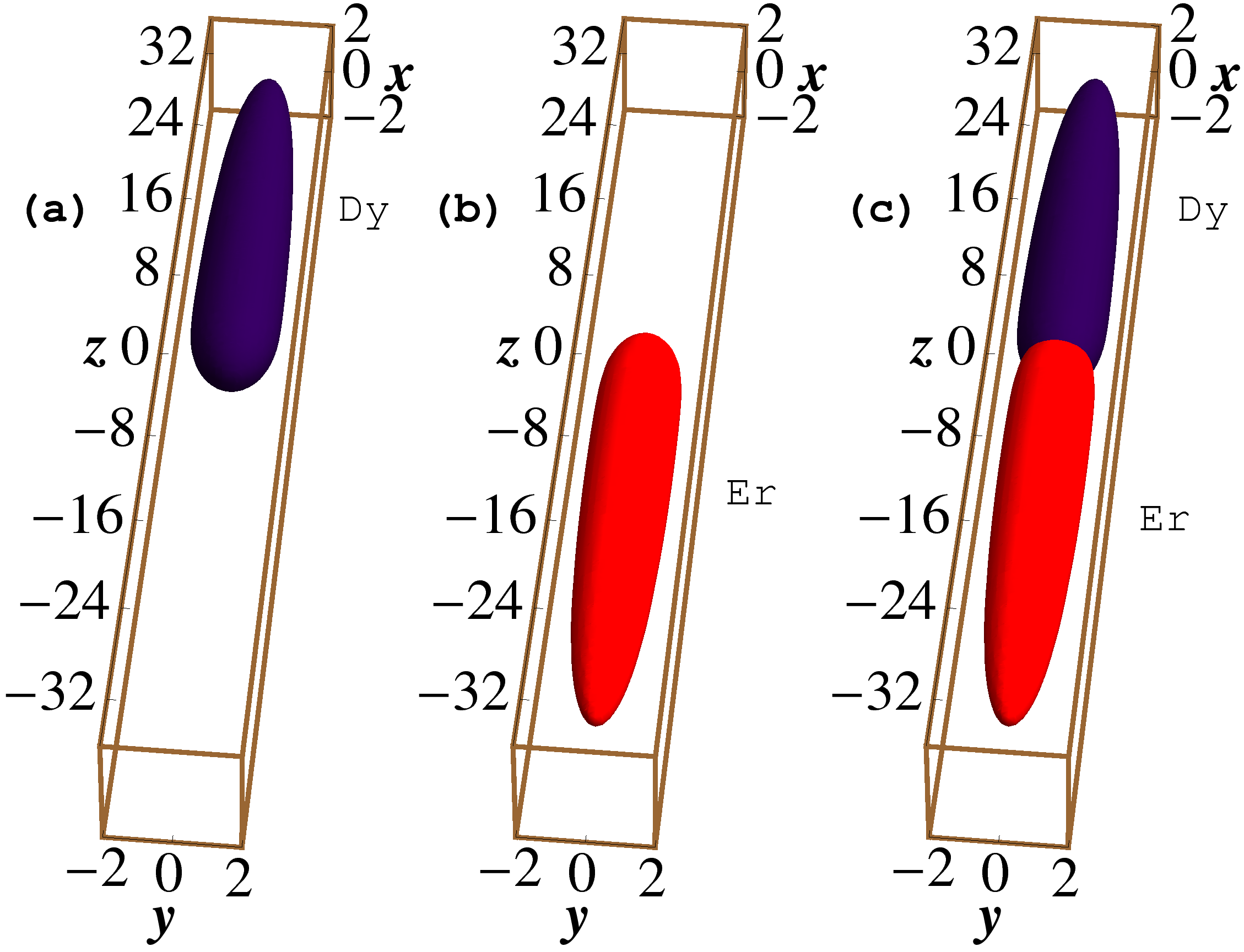
Figure 9: (Color online) Same as in Fig. 3 for the symmetry-broken binary soliton of 2000 ¹⁶⁴Dy and 5000 ¹⁶⁸Er atoms.

The binary dipolar solitons studied above were spatially-symmetric. One can also have symmetry-broken spatially-asymmetric binary solitons for the same parameters used as in the case of spatially-symmetric binary solitons. However, to generate these solitons by imaginary-time propagation one should consider spatially-asymmetric initial states. In particular we consider the following spatial-symmetry broken (asymmetric around $z=0$) initial states with a spatial displacement between the two profiles in imaginary-time propagation:

$$\phi_{1}({\bf r})=\frac{\pi^{-3/4}}{w_{\rho}\sqrt{w}_{z}}\exp\left[-\frac{\rho^{2}}{2w_{\rho}^{2}}-\frac{(z-z_{0})^{2}}{2w_{z}^{2}}\right]$$ (11)

$$\phi_{2}({\bf r})=\frac{\pi^{-3/4}}{w_{\rho}\sqrt{w}_{z}}\exp\left[-\frac{\rho^{2}}{2w_{\rho}^{2}}-\frac{(z+z_{0})^{2}}{2w_{z}^{2}}\right]$$ (12)

in place of the initial states (10). It is important to mention that the imaginary-time propagation converges to the lowest-energy state maintaining the symmetry of the initial state. For example, in the 1D harmonic oscillator problem the imaginary-time propagation with a spatially-symmetric initial state will converge to the ground state of the problem, whereas with a spatially-antisymmetric initial state it will converge to the spatially-antisymmetric first excited state. With the initial states (11) and (12), we obtain the symmetry-broken spatially-asymmetric binary solitons with the same parameters as used in the spatially-symmetric binary solitons. We tried some other forms of symmetry-broken initial state and found that the solution converges always to the same final state. After some experimentation, we could locate for the same set of parameters of the problem only two definite demixed final states: (a) the symmetric states of Figs. 3 and 6 and (b) the symmetry broken states to be presented next.

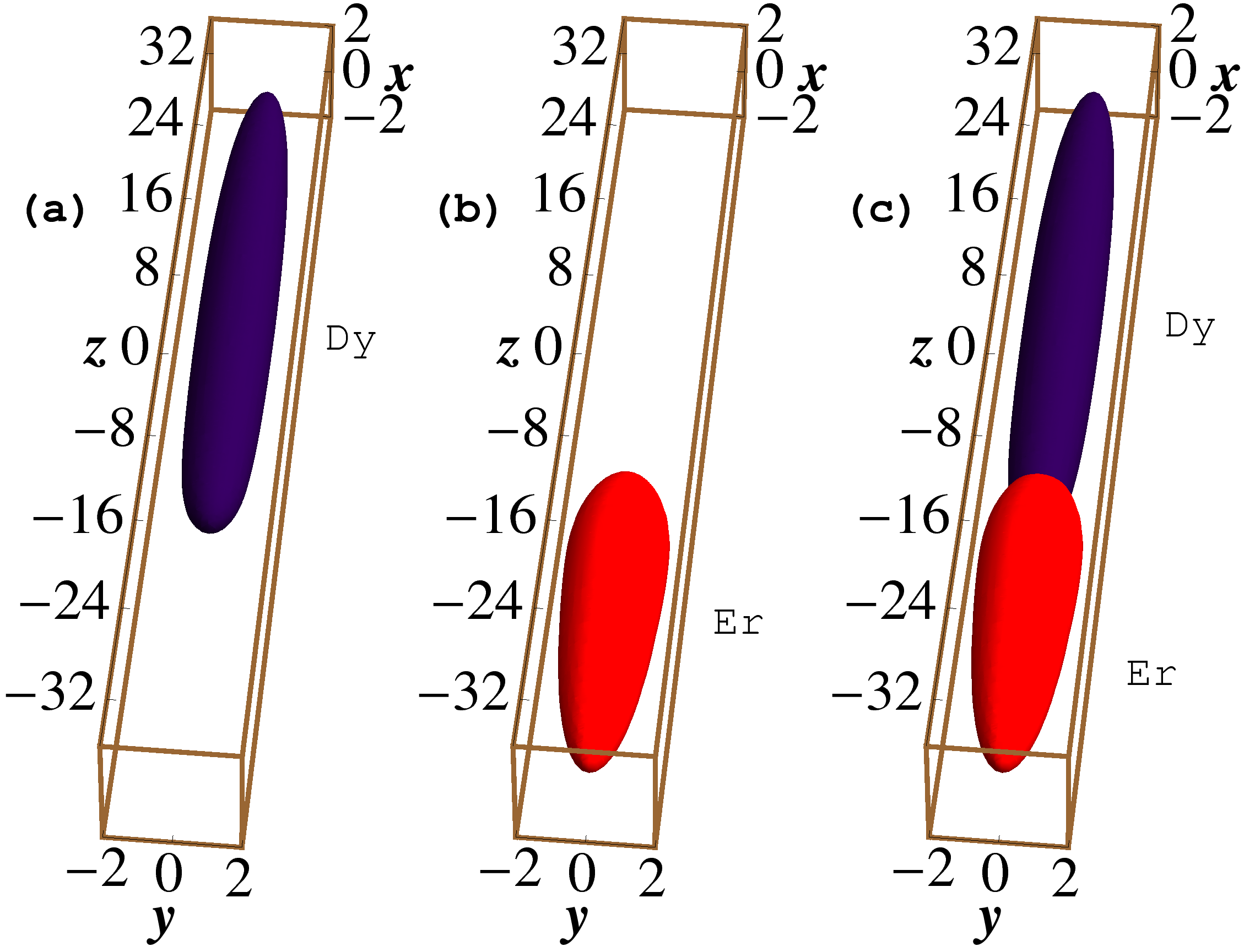
Figure 10: (Color online) Same as in Fig. 3 for the symmetry-broken binary soliton of 5000 ¹⁶⁴Dy and 1000 ¹⁶⁸Er atoms.

We perform imaginary-time propagation with the initial states (11) and (12) using the same parameters as in Fig. 3. The result was insensitive to the value of the parameter $z_{0}$ in Eqs. (11) and (12) and we take $z_{0}=10$ in this study. The 3D isodensity contours of the resultant soliton profiles in this case for 2000 ¹⁶⁴Dy and 5000 ¹⁶⁸Er atoms are shown in Fig. 9. The converged binary dipolar soliton is clearly spatially-asymmetric. The second species with a larger number of ¹⁶⁸Er atoms has a longer spatial extension than the ¹⁶⁴Dy atoms. Then we consider imaginary-time propagation using the same parameters as in Fig. 6. The 3D isodensity contours of the converged state are shown in Fig. 10. In this case with 5000 ¹⁶⁴Dy and 1000 ¹⁶⁸Er atoms the ¹⁶⁴Dy BEC clearly occupies a larger region of space than the ¹⁶⁸Er atoms.

In case of demixed solitons, it is interesting to ask which of the two configurations $-$ symmetric or asymmetric $-$ has the lower energy and hence will be experimentally favorable. To this end we calculated numerically the respective energies in several cases and found that consistently the spatially asymmetric configuration has slightly lower energy. However, this will not be of phenomenological interest as the energy difference is very small, being of the order of 0.1$\%$ of the total energy of either state.

Now we investigate the stability of these symmetry-broken binary dipolar solitons. To this end we consider the converged solutions of the imaginary-time routine and use these as the initial states in real-time routine with the oscillating interspecies scattering length $a_{12}=a($Dy-Er$)=90a_{0}+10a_{0}\cos(t/t_{0})$ as in the case of oscillation presented in Fig. 7. During real-time propagation the system executes small oscillation and the contour plot of the integrated 1D densities is illustrated in Fig. 11. There is no visible change in the widths of the condensates during real-time propagation confirming stability. We also compared the 1D and 3D profiles of the initial and final states (not presented here) and found that they are practically identical.

The demixed binary solitons as presented in Figs. 3, 6, 9, e 10 are ideal examples of soliton molecules of different species where the participating solitons maintain their identities with a minimum of overlap. The binding between the two solitons come from the long-range dipolar interaction. In nondipolar systems such binding can only come from short-range interspecies attraction and a composite soliton molecule can appear possibly only with complete overlap between participating solitons mfb3 ; solmol .

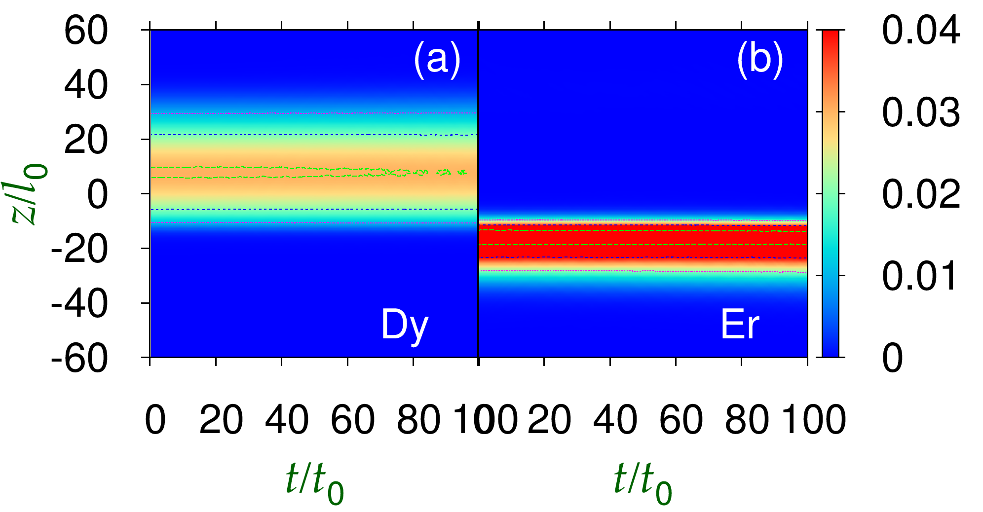
Figure 11: (Color online) Same as in Fig. 7 for the symmetry-broken binary soliton of Fig. 10.

The demixed binary dipolar soliton or the binary soliton molecule can be prepared and observed experimentally. We illustrate the possibility of experimental realization of the soliton shown in Figs. 6 and 9 by realistic numerical simulation using the binary GP Eqs. (7) and (8). In case of the spatially-symmetric binary soliton of Fig. 6 we prepare a spatially-symmetric binary quasi-1D trapped dipolar BEC of 5000 ¹⁶⁴Dy and 1000 ¹⁶⁸Er atoms with the same parameters as in Fig. 6 by imaginary-time simulation but with traps $V({\bf r})=(\rho^{2}/2+\lambda^{2}z^{2}/2)$ and $V({\bf r})=m_{\omega}(\rho^{2}/2+\lambda^{2}z^{2}/2)$ with $\lambda=0.03$, respectively, on ¹⁶⁴Dy and ¹⁶⁸Er atoms, in place of the axially free traps $V({\bf r})=\rho^{2}/2$ and $V({\bf r})=m_{\omega}\rho^{2}/2$. For both ¹⁶⁴Dy and ¹⁶⁸Er atoms these traps correspond to one of axial angular frequency $\omega_{z}=2\pi\times 2$ Hz and of radial angular frequency $\omega_{\rho}=2\pi\times 61$ Hz. This binary bound dipolar BEC is then used as the initial state in the real-time program. During real-time propagation, from $t/t_{0}=0$ to 20 the axial traps $\lambda^{2}z^{2}/2$ are gradually (linearly) reduced to zero, so that for $t/t_{0}>20$ the axially free quasi-1D binary dipolar soliton emerges. The simulation is continued for a long interval of time and a steady propagation of the binary demixed dipolar soliton is established. The outcome of this simulation is shown in Fig. 12 (a), where we plot the integrated 1D density $|\phi_{i}(z,t)|^{2}$ of the two component solitons as obtained from real-time propagation. A similar simulation for the spatially-asymmetric binary soliton of Fig. 9 is shown in Fig. 12 (b). After being released from the axial trap for $t/t_{0}>20$, the solitons expand a little and then oscillate around their appropriate sizes. The stability of the demixed binary dipolar solitons is evident in the simulations illustrated in Figs. 12 (a) and (b).

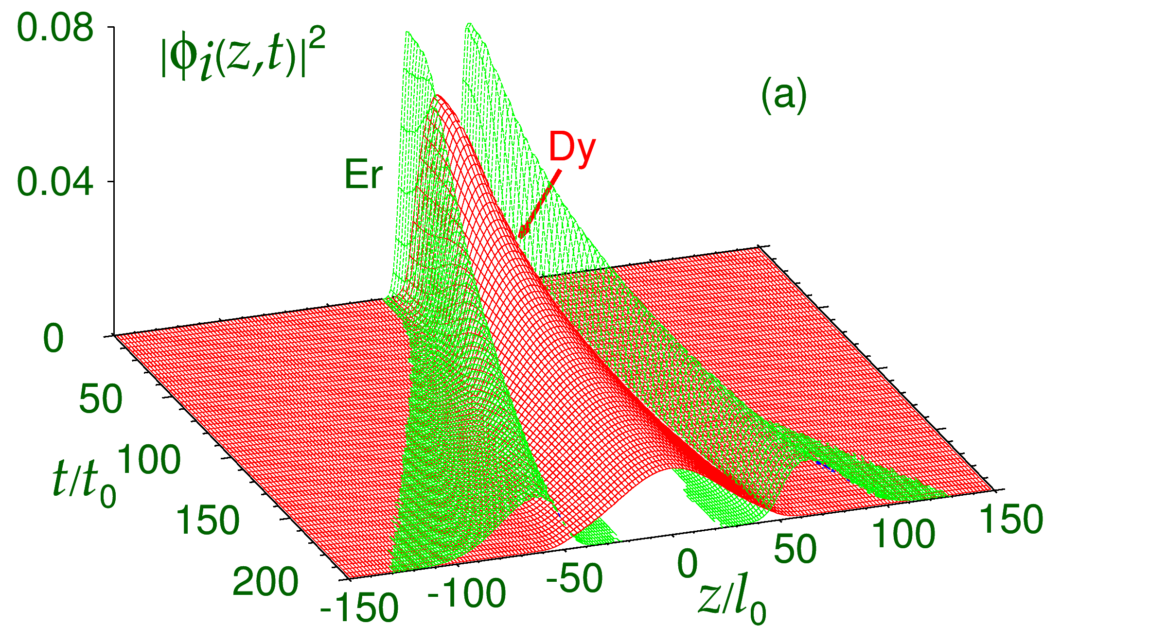
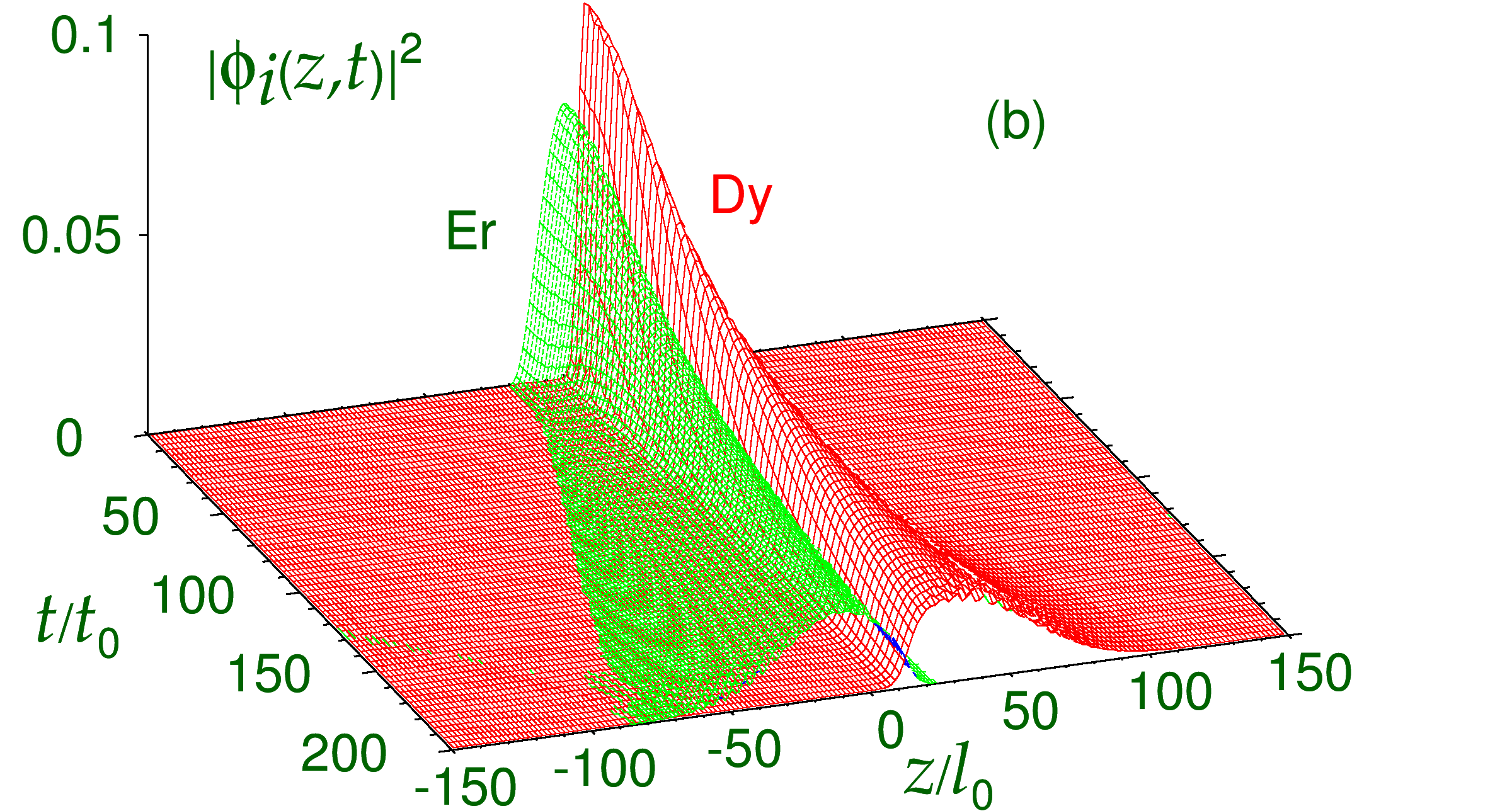
Figure 12: (Color online) Integrated 1D density $|\phi_{i}(z,t)|^{2}=\int dx\int dy|\phi_{i}({\bf r},t)|^{2}$ of ¹⁶⁴Dy (red) and ¹⁶⁸Er (green) atoms during real-time propagation when the axial trap of angular frequency $\omega_{z}=2\pi\times 2$ Hz on a (a) quasi-1D spatially-symmetric binary dipolar BEC of 5000 ¹⁶⁴Dy and 1000 ¹⁶⁸Er atoms and a (b) quasi-1D spatially-asymmetric binary dipolar BEC of 2000 ¹⁶⁴Dy and 5000 ¹⁶⁸Er atoms is removed linearly for $20>t/t_{0}>0$ and the resultant soliton is propagated. Parameters used in simulation: $a($Dy$)=120a_{0},a($Er$)=60a_{0},a($Dy-Er$)=90a_{0},\omega_{\rho}=2\pi\times 61$ Hz, $l_{0}=1$ $\mu$m.

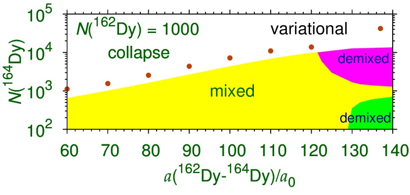
Figure 13: (Color online) Same as in Fig. 4 for a binary ¹⁶⁴Dy-¹⁶²Dy soliton for $N$(¹⁶²Dy) = 1000 atoms. The variational mixed-collapse boundary is indicated by solid circles. For a spatially-symmetric demixed binary soliton, in the upper darker (pink) region the ¹⁶²Dy atoms stay out and in the lower darker (green) region the ¹⁶⁴Dy atoms stay out of the central region. Parameters used: $l_{0}=1$ $\mu$m, $a(^{164}$Dy)= $a(^{164}$Dy)= 120$a_{0}$.

III.3 Binary ¹⁶⁴Dy-¹⁶²Dy soliton

Here we consider yet another type of binary dipolar soliton, e.g. the ¹⁶⁴Dy-¹⁶²Dy soliton. This is particularly interesting as Lev and his collaborators are studying this binary mixture in laboratory levb . In order to permit a large number of atoms in the solitons we consider a large value for the scattering lengths, e.g. $a(^{162}$Dy) = $a(^{164}$Dy) =120$a_{0}$, viz. Fig. 1. The interspecies scattering length is considered as a variable. First we consider the stability phase plot for this binary soliton. In Fig. 13 we show the number of ¹⁶⁴Dy atoms in the binary soliton for 1000 ¹⁶²Dy atoms. Again there appears mixed and demixed binary solitons. As the mass and dipolar lengths are almost the same for the two isotopes the binary plot is quasi symmetric. The plot for 1000 ¹⁶⁴Dy atoms in the binary soliton will lead to a practiaclly identical plot as that in Fig. 13 with the role of the two isotopes interchanged. This system is highly dipolar compared to the ¹⁶⁴Dy-¹⁶⁸Er mixture and hence can accommodate a smaller number of solitons as can be seen by comparing Fig. 13 with Figs. 4 and 5 with 1000 atoms of one of the components. Compared to the ¹⁶⁴Dy-¹⁶⁸Er mixture, demixed binary solitons in ¹⁶⁴Dy-¹⁶²Dy only appears for a larger value of interspecies scattering length to compensate for larger interspecies dipolar attraction. In Figs. 4 and 5 demixing appears for interspecies scattering length $a_{12}\lesssim 100a_{0}$, whereas in Fig. 13 demixing appears for $a_{12}\gtrsim 120a_{0}$.

In this case also one has mixed, spatially-symmetric demixed, and spatial symmetry-broken demixed binary solitons. Without repeating a detailed discussion of different types of solitons, in Fig. 14 we show the isodensity contour of a typical spatially-symmetric binary ¹⁶⁴Dy-¹⁶²Dy soliton for 1000 ¹⁶²Dy atoms and 5000 ¹⁶⁴Dy atoms for the interspecies scattering length $a(^{162}$Dy-¹⁶⁴Dy)=$130a_{0}$. The component ¹⁶²Dy with a smaller number of atoms stays out of the central region whereas the component ¹⁶⁴Dy with a larger number of atoms stays at the center.

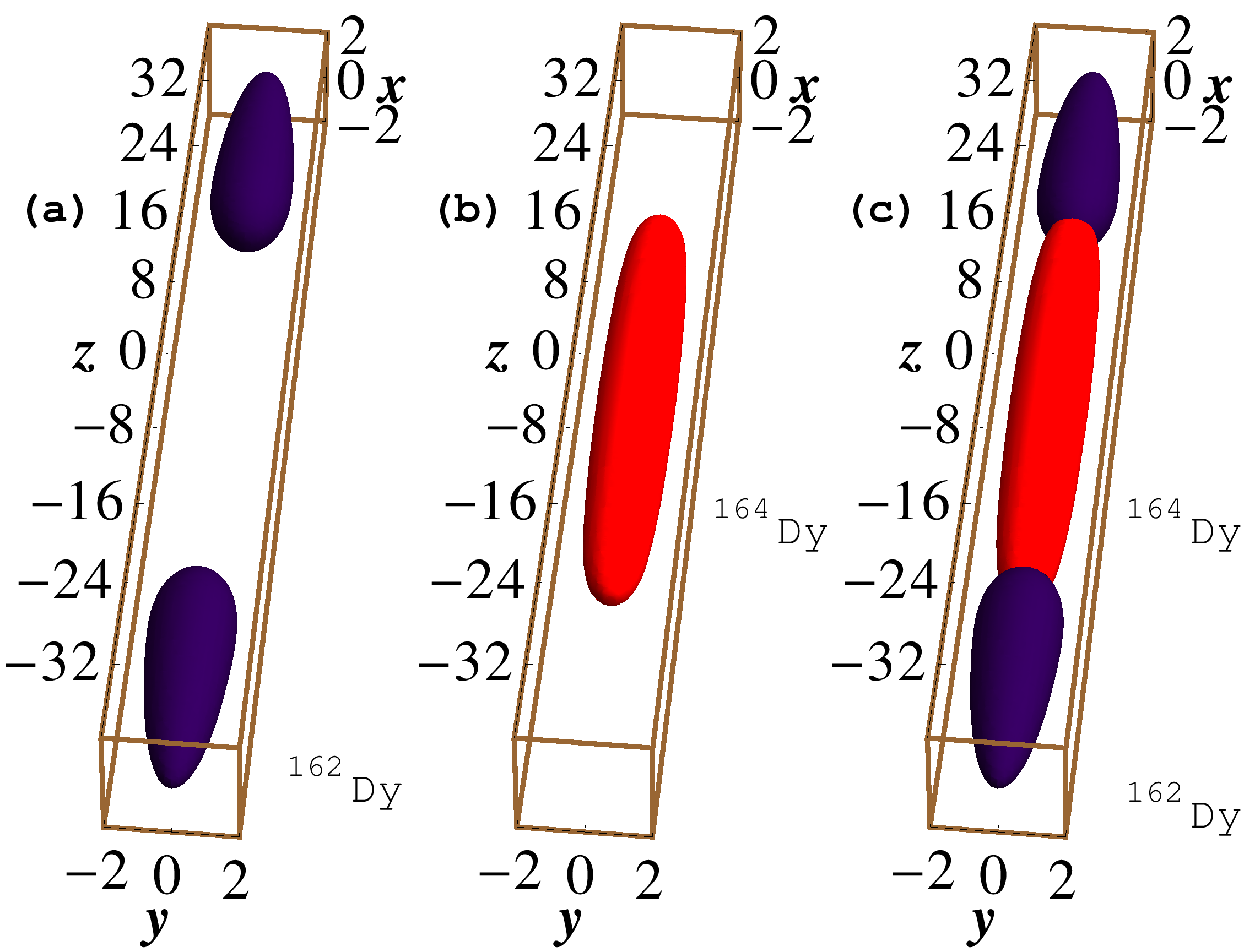
Figure 14: (Color online) 3D isodensity contour (a) $|\phi_{1}|^{2}$ of ¹⁶²Dy, (b) $|\phi_{2}|^{2}$ of ¹⁶⁴Dy, and (c) $(|\phi_{1}|^{2}+|\phi_{2}|^{2})$ of the ¹⁶⁴Dy-¹⁶²Dy mixture for the binary soliton of 1000 ¹⁶²Dy and 5000 ¹⁶⁴Dy atoms with $a(^{162}$Dy$)=a(^{164}$Dy$)=120a_{0},a(^{162}$Dy-¹⁶⁴Dy)=$130a_{0}$. The dimensionless lengths $x,y$ and $z$ are in units of $l_{0}(\equiv 1$ $\mu$m). The density on contour is 0.002.

IV Summary and Discussion

Using the numerical solution of a set of coupled 3D mean-field GP equations, we demonstrate the existence of demixed dipolar binary ¹⁶⁴Dy-¹⁶⁸Er and ¹⁶⁴Dy-¹⁶²Dy solitons stabilized by inter- and intraspecies dipolar interactions in the presence of repulsive inter- and intraspecies contact interactions. The domain of the appearance of the binary soliton is highlighted in stability diagrams of number of atoms in the two components and interspecies scattering length $a_{12}$ for fixed dipolar and intraspecies contact interactions. The binary soliton is stable for a maximum number of atoms beyond which it collapses. For small interspecies interaction $a_{12}$ the binary soliton is mixed and for large $a_{12}$ it is demixed. The mixed-collapse boundary was also calculated using a Gaussian variational approximation mfb3 and was found to be in reasonable agreement with the numerical result. We found two types of demixing in this case: (a) spatially-symmetric and (b) spatial-symmetry-broken demixed binary solitons. In the spatially-symmetric case the species with smaller number of atoms breaks up into two equal parts and the parts leave the central region occupied by the species with larger number of atoms and consolidate on both sides of the BEC component with larger number of atoms as shown in Figs. 3, 6 and 14. In the spatially-asymmetric case, the two solitons move away from each other and finally stabilize side by side as shown in Figs. 9 and 10. The two species of the demixed soliton have a minimum of overlap and are stabilized by dipolar interaction in the presence of reasonably strong contact interaction. Such demixed solitons are not possible in the absence of dipolar interaction. We also tested the stability of the demixed solitons by considering real-time propagation with oscillating scattering length with small amplitude. A stable binary soliton should then execute small oscillations. The converged solution of the binary soliton in imaginary-time propagation is used as the initial state of real-time propagation. The solitons are found to exhibit small oscillation over a long time thus establishing their stability.

The solitons considered in this paper are stabilized by long-range dipolar attraction and short-range contact repulsion. The dipolar interaction is attractive in the axial direction and the dipolar repulsion in the transverse direction is compensated by a harmonic trap. Hence unlike normal BEC solitons stabilized by short-range contact attraction, the present dipolar BECs will be more immune to collapse due to short-range repulsion and can easily accommodate 10000 atoms of the binary ¹⁶⁴Dy-¹⁶⁸Er mixture as can be seen from Figs. 4, 5 and 13. The dipolar ($Na_{\mathrm{dd}}$) and contact ($Na$) nonlinear strengths for such these solitons could be typically $\sim 50$ for 5000 ¹⁶⁴Dy atoms. A nondipolar soliton is created only by contact attraction without any repulsion and is fragile due to collapse instability. In a stable nondipolar soliton, the maximum contact interaction strength is $N|a|\sim 0.6$ 1 ; 3 ; 4 . Thus the dipolar soliton with larger interaction strengths can accommodate a much larger number of atoms than the nondipolar solitons and should be of great experimental interest. A way of experimentally realizing these demixed dipolar solitons is suggested and the viability of this scheme is demonstrated by real-time simulation. First, a quasi-1D demixed binary BEC is to be formed with a weak trap in the axial $z$ direction. Then the axial trap is to be removed linearly in a reasonably short time, while the demixed binary BEC turns into a demixed binary soliton. With the present experimental techniques, such binary dipolar BECs can be observed and the conclusions of this study verified.

- (1) K. E. Strecker, G. B. Partridge, A. G. Truscott, and R. G. Hulet, Nature (London) 417, 150 (2002); L. Khaykovich, F. Schreck, G. Ferrari, T. Bourdel, J. Cubizolles, L. D. Carr, Y. Castin, and C. Salomon, Science 256, 1290 (2002).
- (2) S. L. Cornish, S. T. Thompson, and C. E. Wieman, Phys. Rev. Lett. 96, 170401 (2006).
- (3) V. M. Perez-Garcia, H. Michinel, and H. Herrero, Phys. Rev. A 57, 3837 (1998).
- (4) M. Lu, S. H. Youn, and B. L. Lev, Phys. Rev. Lett. 104, 063001 (2010); J. J. McClelland and J. L. Hanssen, Phys. Rev. Lett. 96, 143005 (2006); S. H. Youn, M. W. Lu, U. Ray, and B. V. Lev, Phys. Rev. A 82, 043425 (2010).
- (5) M. Lu, N. Q. Burdick, Seo Ho Youn, and B. L. Lev, Phys. Rev. Lett. 107, 190401 (2011).
- (6) K. Aikawa et al., Phys. Rev. Lett. 108, 210401 (2012).
- (7) T. Lahaye et al., Nature (London) 448, 672 (2007); A. Griesmaier et al., Phys. Rev. Lett. 97, 250402 (2006).
- (8) J. Stuhler et al., Phys. Rev. Lett. 95, 150406 (2005); K. Goral, K. Rzazewski, and T. Pfau, Phys. Rev. A 61, 051601 (2000); T. Koch et al., Nature Phys. 4, 218 (2008); T. Lahaye et al., Rep. Prog. Phys. 72, 126401 (2009).
- (9) Luis E. Young-S., P. Muruganandam, and S. K. Adhikari, J. Phys. B 44, 101001 (2011).
- (10) S. Giovanazzi, D. O’Dell, and G. Kurizki, J. Phys. B 34, 4757 (2001).
- (11) R. Nath, P. Pedri, and L. Santos, Phys. Rev. Lett. 102, 050401 2009; P. Pedri and L. Santos, Phys. Rev. Lett. 95, 200404 (2005); I. I. Tikhonenkov, B. A. Malomed, and A. Vardi, Phys. Rev. Lett. 100, 090406 (2008); P. Köberle, D. Zajec, G. Wunner, and B. A. Malomed, Phys. Rev. A 85, 023630 (2012); R. Eichler, D. Zajec, P. Köberle, J. Main, and G. Wunner, Phys. Rev. A 86, 053611 (2012); R. Eichler, J. Main, and G. Wunner, Phys. Rev. A 83, 053604 (2011); Ai-Xia Zhang and Ju-Kui Xue, Phys. Rev. A 82, 013606 (2010); V. M. Lashkin, Phys. Rev. A 75, 043607 (2007).
- (12) S. K. Adhikari and P. Muruganandam, J. Phys. B 45, 045301 (2012); I. Tikhonenkov, B. A. Malomed, and A. Vardi, Phys. Rev. A 78, 043614 (2008).
- (13) S. K. Adhikari and P. Muruganandam, Phys. Lett. A 376, 2200 (2012).
- (14) S. Inouye et al., Nature (London) 392, 151 (1998).
- (15) Luis E. Young-S. and S. K. Adhikari, Phys. Rev. A86, 063611 (2012); Phys. Rev. A 87, 013618 (2013).
- (16) S. K. Adhikari and Luis E. Young-S., J. Phys. B 47, 015302 (2014).
- (17) S. K. Adhikari, Phys. Rev. A88, 043603 (2013).
- (18) R. M. Wilson, C. Ticknor, J. L. Bohn, and E. Timmermans, Phys. Rev. A 86, 033606 (2012); H. Saito, Y. Kawaguchi, and M. Ueda, Phys. Rev. Lett. 102, 230403 (2009).
- (19) P. Muruganandam and S. K. Adhikari, Comput. Phys. Commun. 180, 1888 (2009); D. Vudragovic, I. Vidanovic, A. Balaz, P. Muruganandam, and S. K. Adhikari, Comput. Phys. Commun. 183, 2021 (2012).
- (20) K. Goral and L. Santos, Phys. Rev. A. 66, 023613 (2002); S. Yi and L. You, Phys. Rev. A 63, 053607 (2001).
- (21) S. Blatt, T. L. Nicholson, B. J. Bloom, J. R. Williams, J.W. Thomsen, P. S. Julienne, and J. Ye, Phys. Rev. Lett. 107, 073202 (2011).
- (22) S. K. Adhikari, Phys. Lett. A 346, 179 (2005).
- (23) B. L. Lev, private communication, (2013).