Helioseismic and Magnetic Imager Multi-height Dopplergrams

Abstract

We study Doppler velocity measurements at multiple heights in the solar atmosphere using a set of six filtergrams obtained by the Helioseismic magnetic Imager on board the Solar Dynamics Observatory. There are clear and significant phase differences between core and wing Dopplergrams in the frequency range above the photospheric acoustic cutoff frequency, which indicates that these are really “multi-height” datasets.

1 Background

In recent helioseismology studies, photospheric Dopplergrams (i.e., maps of the line-of-sight velocity of the photosphere) obtained by the Helioseismic and Magnetic Imager (HMI; Schou et al. 2012) on board the Solar Dynamics Observatory (SDO; Pesnell et al. 2012) have been used to investigate the solar interior. Multi-height velocity information from observations would be very useful not only for helioseismology analyses (e.g., Nagashima et al. 2009), but also for other purposes, in particular for studies of the energy transport by waves in the solar atmosphere (e.g., Jefferies et al. 2006; Straus et al. 2008, 2009; Kneer & Bello González 2011; Bello González et al. 2010).

2 HMI observation datasets

HMI takes filtergrams at 6 wavelengths (+172.0 mÅ ($I_{0}$), +103.2 mÅ  ($I_{1}$), +34.4 mÅ ($I_{2}$), -34.4 mÅ  ($I_{3}$), -103.2 mÅ  ($I_{4}$), and -172.0 mÅ  ($I_{5}$) ) around the Fe i absorption line at 6173 Å. Standard Dopplergrams provided by the HMI pipeline (Couvidat et al. 2012) are derived from these six filtergrams. The formation height of the HMI Doppler signal is estimated to be about 100 km above the $\tau_{\mathrm{5000\AA}}=1$ surface (Fleck et al. 2011). In this study, instead, we try to create multi-height Dopplergrams from the HMI filtergrams.

The observed Fe i line profile shifts in wavelength because of the SDO orbital motion. Since SDO is in a geosynchronous orbit, the SDO orbital velocity toward the Sun is not constant and the absolute value of its line-of-sight (LOS) velocity towards the Sun reaches up to $\sim 3.5\ \mathrm{km\ s^{-1}}$ (Schou et al. 2012). Figure 1 shows some sample observed line profiles. To create these line profiles we averaged the intensity value at each wavelength over a field of view of $30\ \mathrm{degrees}$ square, and hence, the line shift is basically caused by the observer motion. The vertical dotted line indicates the line shift calculated from the observer LOS velocity in the data headers. We use this observer motion to calibrate the multi-height Dopplergrams.

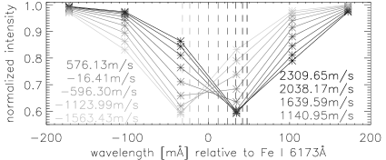
Figure 1.: Sample SDO/HMI observed line profiles. Different gray scales indicate different times, and the numbers on the panel are the observer LOS velocities at these times. The line shift is caused by the spacecraft velocity. The vertical dotted line indicates the line shift calculated from the observer LOS velocity in the data headers.

3 Multi-height Dopplergrams

We calculate three Doppler signals using the set of six filtergrams: $D_{\mathrm{core}}\equiv(I_{3}-I_{2})/(I_{3}+I_{2})$, $D_{\mathrm{wing}}\equiv(I_{4}-I_{1})/(I_{4}+I_{1})$, and $D_{\mathrm{far-wing}}\equiv(I_{5}-I_{0})/(I_{5}+I_{0})$, and convert them into the Doppler velocity, $V_{\mathrm{core}}=f_{\mathrm{core}}(D_{\mathrm{core}})$, $V_{\mathrm{wing}}=f_{\mathrm{wing}}(D_{\mathrm{wing}})$, $V_{\mathrm{far-wing}}=f_{\mathrm{far-wing}}(D_{\mathrm{far-wing}})$. To get the conversion formula, we use the spatial average Doppler signal over a 30-degree-square area near the disc center and the LOS component of SDO observer motion. The functions $f(D)$ are defined by 3rd-order polynomial fitting and the fitting parameters are calculated from three-day observation datasets as shown in Figure 2. Here we use six non-overlapping nine-hour datasets obtained between January 22 0UT and January 24 15UT, 2011, except that we exclude the period from January 22 18UT to January 23 3UT because it has a long data gap. We track 30-degree-square quiet-Sun regions at the Carrington rate for nine hours each using mtrack (Bogart et al. 2011). For each run, the central point of the field of view passes the disc center at the mid-point of the run.

This method to convert the Doppler signal $D$ into the Doppler velocity $V$ is limited within a certain velocity range for two reasons: 1) If the velocity is too large, the Doppler shift of the line is too big and the line center is outside of the blue and red pairs. For the core ($I_{2}$ and $I_{3}$) this limitation is severe; if the velocity exceeds 1.7 km  s^-1 the line center is outside the blue and red pair ($\pm 34.4$ mÅ). 2) Since the SDO motion is less than $\sim 3.5$ km  s ^-1, the fitting is limited within the range.

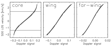
Figure 2.: Scatter plots of mean Doppler signal and the observer LOS velocity. The dotted curves are third-order polynomials and obtained by least-square fitting of the data points. For the core, if the velocity exceeds $1.4\ \mathrm{km\ s^{-1}}$ (solid horizontal lines) the data points are not used for the fitting.

4 Do these Doppler shifts really correspond to velocities at multiple heights?

Correlation coefficients between the Doppler velocities of one snapshot at the time of minimum SDO motion speed on January 23, 2011, are 0.95 ($V_{\mathrm{core}}$ and $V_{\mathrm{wing}}$), 0.83 ($V_{\mathrm{far-wing}}$ and $V_{\mathrm{wing}}$), and 0.76 ($V_{\mathrm{far-wing}}$ and $V_{\mathrm{core}}$). The phase differences between pairs of the Dopplergrams, however, show that $V_{\mathrm{core}}$, $V_{\mathrm{wing}}$, and $V_{\mathrm{far-wing}}$ have promise as multi-height Dopplergrams. Figure 3 shows the phase differences among the three Doppler velocities. Figure 3(c) shows clear phase differences between the wing and core in the frequency range above the photospheric acoustic cutoff frequency ($\sim 5.4$ mHz). The phases referred to the far-wing are noisier (panels (a) and (b)); this might be because the far-wing intensity level is very close to the continuum level, and small fluctuations of the intensity ($I_{0}$ or $I_{5}$) might cause large velocity differences. In the g-mode area (with low frequency and large wavenumber), the sign of the phase difference is opposite to what we have in the higher frequency range; this might be a signature of atmospheric gravity waves, which is consistent with e.g, Straus et al. (2008, 2009). This phase difference also indicates that the two velocities are formed in different heights in the atmosphere.

Mitra-Kraev et al. (2008) used photospheric and chromospheric intensity datasets, instead of Dopplergrams, obtained by the Solar Optical Telescope on board the Hinode satellite. The weak phase shifts above the acoustic cutoff frequency and strong phase shifts in the g-mode area shown in their Figure 1 are consistent with ours, while the strong phase difference along the p-mode ridges which they reported is not seen in our results. The interpretation of the intensity datasets, however, might not be straightforward because of radiation effects. Phase differences between two velocity datasets provide much clearer diagnostics, as they simply measure actual travel times between the two layers.

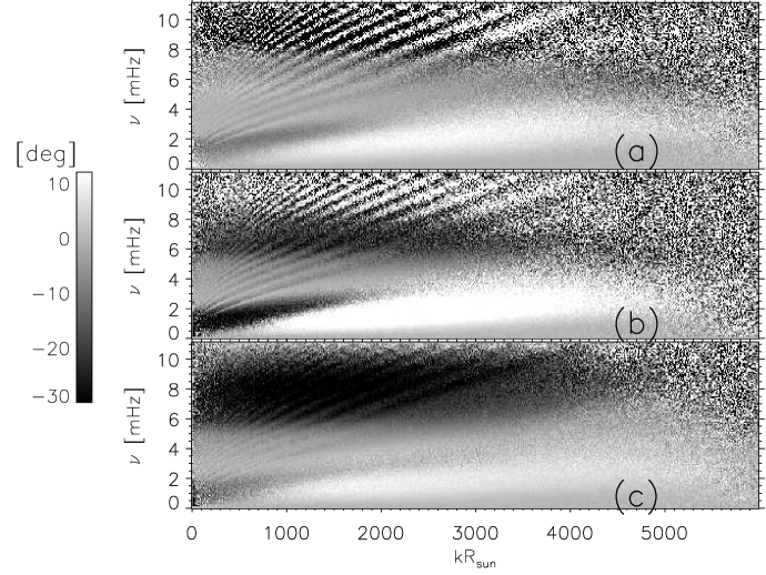
Figure 3.: Phase differences: (a)$\phi_{\mathrm{Far-wing}}-\phi_{\mathrm{Wing}}$, (b) $\phi_{\mathrm{Far-wing}}-\phi_{\mathrm{Core}}$, (c) $\phi_{\mathrm{Wing}}-\phi_{\mathrm{Core}}$. Clear phase differences in the frequency range above the acoustic cutoff frequency are seen in (c).

To estimate the heights of the contribution layers of the multi-height Dopplergrams we plan to use line synthesis calculations in a realistic solar atmospheric model (Nagashima et al. 2013).

Acknowledgments

The HMI data used are courtesy of NASA/SDO and the HMI science team. The German Data Center for SDO, funded by the German Aerospace Center (DLR), provided the IT infrastructure. This work was carried out using the data from the SDO HMI/AIA Joint Science Operations Center Data Record Management System and Storage Unit Management System (JSOC DRMS/SUMS).

References

- Bello González et al. (2010) Bello González, N., Franz, M., Martínez Pillet, V., et al. 2010, ApJ, 723, L134
- Bogart et al. (2011) Bogart, R. S., Baldner, C., Basu, S., Haber, D. A., & Rabello-Soares, M. C. 2011, Journal of Physics Conference Series, 271, 012008
- Couvidat et al. (2012) Couvidat, S., Rajaguru, S. P., Wachter, R., et al. 2012, Solar Phys., 278, 217
- Fleck et al. (2011) Fleck, B., Couvidat, S., & Straus, T. 2011, Solar Phys., 271, 27
- Jefferies et al. (2006) Jefferies, S. M., McIntosh, S. W., Armstrong, J. D., et al. 2006, ApJ, 648, L151
- Kneer & Bello González (2011) Kneer, F., & Bello González, N. 2011, A&A, 532, A111
- Mitra-Kraev et al. (2008) Mitra-Kraev, U., Kosovichev, A. G., & Sekii, T. 2008, A&A, 481, L1
- Nagashima et al. (2009) Nagashima, K., Sekii, T., Kosovichev, A. G., Zhao, J., & Tarbell, T. D. 2009, ApJ, 694, L115
- Nagashima et al. (2013) Nagashima, K., et al. 2013, in prep
- Pesnell et al. (2012) Pesnell, W. D., Thompson, B. J., & Chamberlin, P. C. 2012, Solar Phys., 275, 3
- Schou et al. (2012) Schou, J., Scherrer, P. H., Bush, R. I., et al. 2012, Solar Phys., 275, 229
- Straus et al. (2008) Straus, T., Fleck, B., Jefferies, S. M., et al. 2008, ApJ, 681, L125
- Straus et al. (2009) — 2009, in The Second Hinode Science Meeting: Beyond Discovery-Toward Understanding, edited by B. Lites, M. Cheung, T. Magara, J. Mariska, & K. Reeves, vol. 415 of Astronomical Society of the Pacific Conference Series, 95