Flux Phase as Possible Time-Reversal Symmetry Breaking Surface States of High-$T_{C}$ Cuprate Superconductors

Abstract

At a (110) surface of a $d_{x^{2}-y-2}$-wave superconductor, superconducting order is strongly suppressed. In such a situation, ordered states that are forbidden in the bulk may arise. This problem is studied for high-$T_{C}$ cuprate superconductors by treating the $t-J$ model with extended transfer integrals using the Bogoliubov de Gennes method. It is found that a flux phase with staggered currents along the surface, or an antiferromagnetic state can occur near the surface. Stability of the emergent surface states is different from system to system depending on the shapes of their Fermi surfaces. Possible relation to the experiments on the Kerr effect that suggest time-reversal symmetry breaking is discussed.

1 Introduction

In high-$T_{C}$ cuprate superconductors, the competition and coexistence of several kinds of ordered states are important issues to clarify the mechanism of superconductivity. In high-$T_{C}$ cuprates, superconducting (SC) and antiferromagnetic (AF) states can occur depending on the doping rate ($\delta$). Previously these two states were thought to be exclusive, but it has recently been found that, in multilayer cuprate systems (in this paper the term ”multilayer” will refer to three or more layers in a unit cell), they can coexist uniformly in the same CuO₂ plane.[1]

Whether ordered states other than the SC and AF states exist in high-$T_{C}$ cuprates is a subtle question concerning the pseudogap phase in the underdoped region. [2, 3] In principle, a state that has a free energy higher than other states cannot occur, but it may arise if the stable ordered state is suppressed due to some reason. For example, near a (110) surface of a $d_{x^{2}-y^{2}}$-wave superconductor, SC order is strongly suppressed. In such a case other states forbidden in the bulk, e.g. a flux phase may arise. The flux phase is a mean-field (MF) solution to the $t-J$ model on a square lattice that describes the low-energy electronic states of high-$T_{C}$ cuprates.[4, 5] In this state the staggered circulating currents flow and a flux $\phi$ penetrates the plaquette in a square lattice.[4] Near (away from) half filling $\phi=\pm\pi$ ($\phi\not=\pm\pi$) and the state is called the $\pi$-flux (staggered-flux) phase. (The $d$-density wave states, which have been introduced in a different context, have similar properties.[6])

Although the flux phase is only metastable except very near half-filling,[7, 8] it is energetically close to the SC state. Bejas et al. treated the $t-J$ model with a second-neighbor hopping term using $1/N$ expansion in the leading order. In this treatment, the SC and AF states are excluded, and they found that the flux phase is the leading instability even at high doping rates.[9] A mean-field (MF) calculation based on the slave-boson (SB) scheme[10, 11] for the $t-J$ model with second- and third- nearest-neighbor hopping terms (extended $t-J$ model) has been carried out to estimate the bare transition temperature of the flux phase, $T_{FL}$, assuming the absence of SC order.[12] It turned out that $T_{FL}$ may be finite even for a large doping rate ($\delta\lesssim 0.15$).

When the flux phase occurs near the (110) surface of the $d_{x^{2}-y^{2}}$-wave superconductor, the circulating current in the flux phase becomes a staggered current flowing along the surface with an amplitude decaying toward the bulk. This means that the time-reversal symmetry (${\cal T}$) is broken locally near the surface. Experimentally, nonzero Kerr rotations have been observed in high-$T_{C}$ cupates,[13, 14, 15] and it may be considered as the sign of the ${\cal T}$ violation. To explain these experiments, several theories have been proposed.[16, 17, 18, 19, 20] We will examine whether the Kerr effect experiments can be explained by the flux phase near the surface.

Another possible surface state at the (110) surface of the $d_{x^{2}-y^{2}}$-wave superconductor is the AF state. Relative stability of the flux phase and the AF state as the emergent surface state depends on the dimensionality of the system as well as the shapes of their Fermi surfaces (FSs). In purely two-dimensional systems, the AF state cannot occur, because rotational symmetry in spin space would be broken spontaneously in the AF state. (In contrast, only discrete symmetry is broken in the flux phase.) The AF state can be stabilized by a weak three dimensionality that is always present in real systems. In single or double layer cuprates, three dimensionality is so weak that the AF state appears only near half-filling. For a La_2-xSr_xCuO₄ (LSCO) system (single layer), the critical doping rate of the AF state is $\delta_{c}^{AF}\sim 0.02$,[21] and for a YBa₂Cu₃O_6+x (YBCO) system (bilayer) $\delta_{c}^{AF}\sim 0.05$.[22] On the other hand, in multilayer systems, the AF order survives up to a rather large doping region ($\delta_{c}^{AF}\sim 0.1$)[1] due to the relatively strong three dimensionality. This implies that, in single and bilayer cuprates, the flux phase may be favorable as the surface state. The surface AF order may be expected in multilayer cuprate systems for a doping range where only the SC order exists in the bulk. As we will see in the following, the shape of the FS is also responsible for the stability.

In this paper we study the states near (110) surfaces of $d_{x^{2}-y^{2}}$-wave superconductors that are described by the extended $t-J$ model. The spatial variations of the order parameters (OPs) are treated using the Bogoliubov de Gennes (BdG) method[23] based on the SBMA approximation. The long-range hopping terms are introduced to represent the different shapes of FSs for various high-$T_{C}$ cuprate superconductors. We will show that the flux phase or the AF state can occur as surface states, and their relative stability will be discussed.

This paper is organized as follows. In Sect. 2 the model is presented and the BdG equations are derived. Results of numerical calculations for the surface states are described in Sect. 3. In Sect 4 the local density of states is examined. Section 5 is devoted to summary and discussion.

2 Bogoliubov de Gennes Equations

We consider the $t-J$ model on a square lattice whose Hamiltonian is given as

$$\displaystyle H=-\sum_{jl\sigma}t_{jl}{\tilde{c}}^{\dagger}_{j\sigma}{\tilde{c}}_{l\sigma}+J\sum_{\langle j,l\rangle}{\bf S}_{j}\cdot{\bf S}_{l},$$ (1)

where the transfer integrals $t_{jl}$ are finite for the first- ($t$), second- ($t^{\prime}$), and third-nearest-neighbor bonds ($t^{{}^{\prime\prime}}$), or zero otherwise. $J(>0)$ is the antiferromagnetic superexchange interaction and $\langle j,l\rangle$ denotes the nearest-neighbor bonds. ${\tilde{c}}_{j\sigma}$ is the electron operator in Fock space without double occupancy, and we treat this condition using the SB method[10, 11] by writing ${\tilde{c}}_{j\sigma}=b_{j}^{\dagger}f_{j\sigma}$ under the local constraint $\sum_{\sigma}f_{j\,\sigma}^{\dagger}f_{j\,\sigma}+b_{j}^{\dagger}b_{j}=1$ at every $j$ site. Here $f_{j\sigma}$ ($b_{j}$) is a fermion (boson) operator that carries spin $\sigma$ (charge $e$); the fermions (bosons) are frequently referred to as spinons (holons). The spin operator is expressed as ${\bf S}_{j}=\frac{1}{2}\sum_{\alpha,\beta}f^{\dagger}_{j\alpha}{\bf\sigma}_{\alpha\beta}f_{j\beta}$.

We decouple the Hamiltonian Eq. (1) in the following manner.[24, 25, 26, 27, 28] The bond order parameters $\langle f^{\dagger}_{j\sigma}f_{l\sigma}\rangle$ and $\langle b^{\dagger}_{j}b_{l}\rangle$ are introduced, and we denote $\chi_{jl\sigma}\equiv\langle f^{\dagger}_{j\sigma}f_{l\sigma}\rangle$ for nearest-neighbor bonds. Although the bosons are not condensed in purely two-dimensional systems at finite temperature ($T$), they are almost condensed at low $T$ and for finite carrier doping ($\delta\gtrsim 0.05$). Since we are interested in the region $\delta\gtrsim 0.05$ and low temperatures, we will treat holons as Bose condensed. Hence we approximate $\langle b_{j}\rangle\sim\sqrt{\delta}$ and $\langle b^{\dagger}_{j}b_{l}\rangle\sim\delta$, and replace the local constraint with a global one, $\frac{1}{N}\sum_{j,\sigma}\langle f^{\dagger}_{j\sigma}f_{j\sigma}\rangle=1-\delta$, where $N$ is the total number of lattice sites. The spin-singlet resonating-valence-bond (RVB) OP on the bond $\langle j,l\rangle$ is given as $\Delta_{j,l}=\langle f_{j\uparrow}f_{l\downarrow}-f_{j\downarrow}f_{l\uparrow}\rangle/2$. Under the assumption of the Bose condensation of holons, $\Delta_{j,l}$ is equivalent to the SCOP. (Then the onset temperature of $\Delta$ is the SC transition temperature, $T_{C}$.) The magnetization is defined by $m_{j}=\langle n_{j\uparrow}-n_{j\downarrow}\rangle/2$ with $n_{j\sigma}=f^{\dagger}_{j\sigma}f_{j\sigma}$.

The phase diagram in the plane of $\delta$ and $T$, obtained within the SBMF approximation, can describe the SC and AF states qualitatively.[26, 27, 28] In a quantitative sense, however, the region of the AF state is overestimated. The discrepancy is due to the MF treatment, and it could be remedied by the inclusion of fluctuations. However, to treat the fluctuations within the BdG calculation is beyond the scope of this work, we introduce a phenomenological parameter $r$ ($0<r\leq 1$) to suppress the AF order:[29, 30] in the decoupling procedure of the $J$ term, $J\langle{\bf S}_{j}\rangle\cdot{\bf S}_{l}$ is replaced by $rJ\langle{\bf S}_{j}\rangle\cdot{\bf S}_{l}$.

When the SC and AF order coexists, the so-called $\pi$-triplet pairing can occur.[31, 32, 33, 34, 35] In this paper we neglect them for simplicity, because their amplitude is much smaller than that of the singlet SCOP.

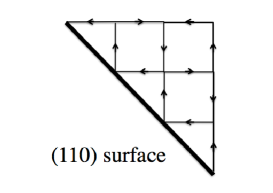
Figure 1: Schematic of a (110) surface. Arrows indicate directions of currents.

We treat a system with a (110) surface (Fig.1), and denote the direction perpendicular (parallel) to the (110) surface as $x$ ($y$). The $x$ coordinate is given as $x=j_{x}a$ where $a=a^{\prime}/\sqrt{2}$ with $a^{\prime}$ being the lattice constant of the square lattice. In order to describe the Flux phase and the $d$-wave SC state, $\chi^{(\pm)}_{j\sigma}\equiv\chi_{j,j+x\pm y,\sigma}$ and $\Delta^{(\pm)}_{j}\equiv\Delta_{j.j+x\pm y}$ are defined. We assume that the system is uniform along the $y$ direction, and consider the spatial variations of OPs only in the $x$ direction. By imposing the periodic boundary condition for the $y$ direction, the Fourier transformation for the $y$ coordinate is performed.[36, 37, 38, 39] (Hereafter we write $j_{x}$ simply as $j$.) Then the mean-field Hamiltonian is written as follows

$${\cal H}_{MF}=\sum_{k}\sum_{j,l}\Psi_{j}^{\dagger}(k){\hat{h}}_{jl}(k)\Psi_{l}(k),$$ (2)

with $\displaystyle\Psi_{j}^{\dagger}(k)=\big{(}f_{j\uparrow}^{\dagger}(k),f_{j\downarrow}(-k)\big{)}$, and $k$ is the wave number along the $y$ direction. The matrix ${\hat{h}}_{ij}(k)$ is given as

$${\hat{h}}_{jl}(k)=\left(\begin{array}[]{cc}\xi_{jl\uparrow}(k)&F_{jl}(k)\\ F_{lj}^{*}(k)&-\xi_{jl\downarrow}(k)\end{array}\right),$$ (3)

where

$$\begin{array}[]{rl}\xi_{jl\uparrow}(k)=&\displaystyle-\delta_{j,l}\big{[}\mu-rJ(m_{j-1}+m_{j+1})+2t^{\prime}\delta\cos 2ka\big{]}\\ &\displaystyle-\delta_{j,l-1}\big{[}2t\delta\cos ka+\frac{J}{2}[(\chi^{(+)}_{j\downarrow}+\frac{1}{2}\chi^{(+)}_{j\uparrow})e^{ik}\\ &\displaystyle+(\chi^{(-)}_{j\downarrow}+\frac{1}{2}\chi^{(-)}_{j\uparrow})e^{-ik}]\big{]}\\ &\displaystyle-\delta_{j,l+1}\big{[}2t\delta\cos ka+\frac{J}{2}[(\chi^{(+)}_{l\downarrow}+\frac{1}{2}\chi^{(+)}_{l\uparrow})^{*}e^{-ik}\\ &\displaystyle+(\chi^{(-)}_{l\downarrow}+\frac{1}{2}\chi^{(-)}_{l\uparrow})^{*}e^{ik}]\big{]}\\ &\displaystyle-(\delta_{j,l+2}+\delta_{j,l-2})(t^{\prime}\delta+2t^{\prime\prime}\delta\cos 2ka),\\ &\\ \xi_{jl\downarrow}(k)=&\displaystyle-\delta_{j,l}\big{[}\mu+rJ(m_{j-1}+m_{j+1})+2t^{\prime}\delta\cos 2ka\big{]}\\ &\displaystyle-\delta_{j,l-1}\big{[}2t\delta\cos ka+\frac{J}{2}[(\chi^{(+)}_{j\uparrow}+\frac{1}{2}\chi^{(+)}_{j\downarrow})^{*}e^{ik}\\ &\displaystyle+(\chi^{(-)}_{j\uparrow}+\frac{1}{2}\chi^{(-)}_{j\downarrow})^{*}e^{-ik}]\big{]}\\ &\displaystyle-\delta_{j,l+1}\big{[}2t\delta\cos ka+\frac{J}{2}[(\chi^{(+)}_{l\uparrow}+\frac{1}{2}\chi^{(+)}_{l\downarrow})e^{-ik}\\ &\displaystyle+(\chi^{(-)}_{l\uparrow}+\frac{1}{2}\chi^{(-)}_{l\downarrow})e^{ik}]\big{]}\\ &\displaystyle-(\delta_{j,l+2}+\delta_{j,l-2})(t^{\prime}\delta+2t^{\prime\prime}\delta\cos 2ka),\\ &\\ F_{jl}(k)=&\displaystyle\frac{3J}{4}\big{[}\delta_{j,l-1}(\Delta^{(+)}_{j}e^{ika}+\Delta^{(-)}_{j}e^{-ika})\\ +&\displaystyle\delta_{j,l+1}(\Delta^{(+)}_{l}e^{-ika}+\Delta^{(-)}_{l}e^{ika})\big{]},\end{array}$$ (4)

with $\mu$ being the chemical potential,

We diagonalize the mean-field Hamiltonian by solving the following BdG equation for each $k$,

$$\sum_{l}{\hat{h}}_{jl}(k)\left(\begin{array}[]{cc}u_{ln}(k)\\ v_{ln}(k)\end{array}\right)=E_{n}(k)\left(\begin{array}[]{cc}u_{jn}(k)\\ v_{jn}(k)\end{array}\right),$$ (5)

where $E_{n}(k)$ and ($u_{jn}(k)$, $v_{jn}(k)$) are the energy eigenvalue and the corresponding eigenfunction, respectively, for each $k$. The unitary transformation using ($u_{jn}(k)$, $v_{jn}(k)$) diagonalizes the Hamiltonian ${\cal H}_{MF}$, and the OPs and the spinon number at the $j$ site can be written as,

$$\begin{array}[]{rl}\langle n_{j\uparrow}\rangle=&\displaystyle\frac{1}{N_{y}}\sum_{k}\sum_{n=1}^{2N_{x}}\big{|}u_{j,n}(k)\big{|}^{2}f(E_{n}(k)),\\ \langle n_{j\downarrow}\rangle=&\displaystyle\frac{1}{N_{y}}\sum_{k}\sum_{n=1}^{2N_{x}}\big{|}v_{j,n}(k)\big{|}^{2}\big{[}1-f(E_{n}(k))\big{]},\\ \chi^{(\pm)}_{j\uparrow}=&\displaystyle\frac{1}{N_{y}}\sum_{k}\sum_{n=1}^{2N_{x}}e^{\mp ika}u^{*}_{j+1.n}(k)u_{j,n}(k)f(E_{n}(k)),\\ \chi^{(\pm)}_{j\downarrow}=&\displaystyle\frac{1}{N_{y}}\sum_{k}\sum_{n=1}^{2N_{x}}e^{\pm ika}v_{j+1.n}(k)v^{*}_{j,n}(k)\big{[}1-f(E_{n}(k))\big{]},\\ \Delta^{(\pm)}_{j}=&\displaystyle\frac{1}{4N_{y}}\sum_{k}\sum_{n=1}^{2N_{x}}\big{[}e^{\mp ika}u_{j,n}(k)v^{*}_{j+1,n}(k)\\ &\displaystyle+e^{\pm ika}u_{j+1,n}(k)v^{*}_{j,n}(k)\big{]}\tanh\Big{(}\frac{E_{n}(k)}{2T}\Big{)},\end{array}$$ (6)

where $N_{x}$ ($N_{y}$) and $f$ are the number of lattice sites along the $x$ ($y$) direction and the Fermi distribution function, respectively. The $d$- and $s$-wave SCOPs are obtained by combining $\Delta^{(\pm)}$s: $\Delta_{d}(j)=(\Delta^{(+)}_{j}-\Delta^{(-)}_{j}+\Delta^{(+)}_{j-1}-\Delta^{(-)}_{j-1})/4$ and $\Delta_{d}(j)=(\Delta^{(+)}_{j}+\Delta^{(-)}_{j}+\Delta^{(+)}_{j-1}+\Delta^{(-)}_{j-1})/4$.

3 Surface States

In this section we present the results of numerical calculations for surface states. Spatial variations of the OPs near (110) surfaces are determined by solving the BdG equations, and we restrict ourselves to the case of $T<T_{C}$, namely, we do not consider the pseudogap phase. In numerical calculations, we diagonalize the Hamitotonian ${\cal H}_{MF}$ with the OPs substituted in matrix elements, and the resulting eigenvalues and eigenfunctions are used to recalculate the OPs. This procedure is iterated until the convergence is reached. For the system size, $N_{x}=200$ and $N_{y}=100$ are used throughout.

First we study the LSCO system. The transfer integrals are chosen to reproduce the FS of the LSCO system, $t/J=4$, $t^{\prime}/t=-1/6$, and $t^{\prime\prime}=0$,[40] and $\delta=0.10$ and $T=0.01J$ are used. In the LSCO system, the region of the AF state is very narrow ($\delta\lesssim 0.02$), and we do not consider it. In Fig.2, the spatial variations of the OPs are shown. It is seen that the $d$-wave SCOP $\Delta_{d}$ is suppressed near the surface ($x=0$), and the imaginary part of the bond OP, Im$\chi$, is finite in this region. (In the absence of magnetic order, $\chi_{\uparrow}=\chi_{\downarrow}$.) This mean that the flux phase arises as a surface state and the time-reversal symmetry is broken locally near the surface. The critical value of the doping rate for the appearance of the flux phase, $\delta_{c}$, in the LSCO system is $\delta_{c}\sim 0.20$. In the SBMA calculation for a uniform system, the bare transition temperature of the flux phase, $T_{FL}$, vanishes at $\delta\sim 0.15$.[12] Thus, $\delta_{c}$ in the BdG calculation is larger than that for the uniform system, because the incommensurate flux order that is not taken into account in the latter may be possible.

Next we examine the YBCO system. We use a simplified parametrization of the transfer integrals neglecting bilayer splitting of the FS, $t/J=4$, $t^{\prime}/t=-1/6$, and $t^{\prime\prime}/t=1/5$,[40] and $\delta=0.06$ and $T=0.01J$ are used. (We do not consider the AF state as in the LSCO system.) In Fig.3 the spatial variations of the OPs are shown, and we see that the flux phase and hence the ${\cal T}$ violation also occur in this system. The value of Im$\chi$ that characterizes the flux phase is smaller compared with that in Fig.2, though the doping rate is smaller here. For the YBCO system, $\delta_{c}\sim 0.10$ in the BdG calculation, while $\delta_{c}\sim 0.08$ in the MF calculation for the uniform system.

Figure 2: (Color online) Spatial variations of the OPs for the LSCO system ($t/J=4$, $t^{\prime}/t=-1/6$, $t^{\prime\prime}=0$, $\delta=0.10$, and $T=0.01J$). Here $x$ is measured in units of lattice spacing $a$. Note that all OPs are nondimensional.

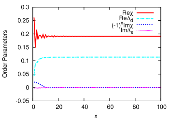
Figure 3: (Color online) Spatial variations of the OPs for the YBCO system ($t/J=4$, $t^{\prime}/t=-1/6$, $t^{\prime\prime}/t=1/5$, $\delta=0.06$, and $T=0.01J$).

The Flux phase arises in a rather large doping range for the LSCO compared to the YBCO system. The reason for the difference is as follows. Flux phases are characterized by the imaginary part of the bond OP, Im$\chi$. Self-consistency equations for the uniform system show that the expression of Im$\chi$ has a form factor $(\gamma_{k}^{(-)})^{2}$ ($\gamma_{k}^{(\pm)}\equiv\cos k_{x}\pm\cos k_{y}$).[7, 8, 12] Therefore, if $(\gamma_{k}^{(-)})^{2}$ is large near the FS, the flux phase should be favored. [12] The FS of the LSCO (YBCO) system is favorable (unfavorable) in this sense.

When the flux phase occurs, it is seen that the imaginary part of the $s$-wave SCOP becomes finite near the surface, and thus the SC state has a $(d\pm is)$-wave symmetry. However, the absolute value of Im$\Delta_{s}$ is very small (of the order of $10^{-3}$), and it is considered to be driven by the flux phase order. The absence of the $s$-wave SCOP, when the flux phase is not present, can be understood by using the Ginzburg-Landau (GL) theory. The coefficient of the quadratic term of the $d$- ($s$-) wave SCOP, $\alpha_{d}$ ($\alpha_{s}$), in the GL theory has been derived microscopically from the $t-J$ model.[41] The $d$- ($s$-) wave SCOP is characterized by the form factor $(\gamma_{k}^{(-)})^{2}$ ($(\gamma_{k}^{(+)})^{2}$), and if $(\gamma_{k}^{(-)})^{2}$ ($(\gamma_{k}^{(+)})^{2}$) is large near the FS, the $d$- ($s$-) wave SC state is favored. For the parameters used in the present BdG calculations, $\alpha_{s}$ is positive both for the LSCO and YBCO systems at least for $T\geq 10^{-4}J$. In general, surface scatterings may induce Re$\Delta_{s}$, but not Im$\Delta_{s}$. Moreover, for (110) surfaces this contribution vanishes by symmetry.[42] Therefore, even when $\Delta_{d}$ is suppressed near the (110) surface, $\Delta_{s}$ would not be induced, because no energy gain is expected.

Although we have considered only (110) surfaces, we may expect ${\cal T}$ violation for surfaces with other types of orientations. In real systems surfaces will not be so smooth, then there may be small domains where the angle of crystal axes is 45^∘ to the surface. In this case the flux phase would appear leading to ${\cal T}$ violation locally in these domains. For a surface perpendicular to the $c$ axis, grain boundaries could also be the origin of the flux phase order.

The current along the surface ($y$ axis) is proportional to Im$\chi$,

$$J_{y}(j)=\frac{\sqrt{2}\pi t\delta}{\phi_{0}}\sum_{\sigma}{\rm Im}\chi^{(+)}_{j\sigma},$$ (7)

with $\phi_{0}=h/2e$ being the flux quantum. (In principle, there is a term proportional to the vector potential in $J_{y}$, but we neglect it for simplicity.) Then the staggered current $J_{y}$ flows in the region where the flux phase order is present. The magnetic field at the surface can be roughly estimated by $B_{z}(x=0)=\mu_{0}\int_{0}^{\infty}dxJ_{y}(x)=\mu_{0}a\sum_{j}J_{y}(j).$ For the parameters used above (corresponding to those in Figs. 2 and 3), $B_{z}(x=0)$ is of the order of 1-10 G. The estimated value of $B$ is small but finite, then it could lead to a finite but small Kerr angle observed experimentally.

The Kerr angles at the opposite surfaces have the same sign,[15] in contradiction to uniform ${\cal T}$ violation. In the present theory, since the ${\cal T}$ violation occurs only near the surface, the signs of the Kerr angles at the opposite sides of the sample can be arbitrary. Therefore it may give a simple explanation for the experimental finding.

Theoretically, the surface flux order can occur only below $\delta_{c}\sim 0.10$ for the YBCO system, and this doping rate is less than the value for which the Kerr rotation is observed in the SC region.[13] The reason for the discrepancy could be due to the fact that we have used the single-layer (single-band) $t-J$ model. If the bilayer $t-J$ model is employed, there are multiple FSs, and the condition for the occurrence of the flux phase may be changed.

In contrast to the LSCO and YBCO systems, the AF state survives up to large $\delta$ in multilayer cuprate superconductors in which the coexistence of the AF and SC states has been found. For example, $T_{N}$ vanishes at $\delta_{c}^{AF}\sim 0.1$ for five-layer cuprate systems.[1] In a state with $\delta\gtrsim\delta_{c}^{AF}$, AF order is suppressed by SC order, though the bare transition temperature of the former, $T_{N}^{bare}$, is still finite. When SC order is suppressed near the (110) surface, there is a competition between the AF state and the flux phase. Here we use the single-layer $t-J$ model for simplicity ($t/J=4$, $t^{\prime}=t^{\prime\prime}=0$), and choose $r=0.66$. For this value of $r$, $T_{N}$ vanishes at $\delta_{c}^{AF}\sim 0.10$. In Fig. 4, the results for $\delta=0.11$ ($>\delta_{c}^{AF}$) and $T=0.01J$ are shown. It is seen that the staggered magnetization $M(=(-1)^{x}m)$ is finite near the surface, while Im$\chi=0$ everywhere. This means that the AF state is more robust than the flux phase in this system. For larger values of $\delta$, surface AF order diminishes, and the flux phase may appear. The above results indicate that the emergent surface state may be different from system to system, depending on the shapes of the FSs.

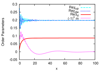
Figure 4: (Color online) Spatial variations of the OPs for the system near the coexistence of the SC and AF states ($t/J=4$, $t^{\prime}=t^{\prime\prime}=0$, $r=0.66$, $\delta=0.11$, and $T=0.01J$).

4 Local Density of States

The local density of states (LDOS) at the $j$ site is given as

$$\begin{array}[]{rl}N_{\uparrow}(j,E)=&\displaystyle\frac{1}{N_{y}}\sum_{k}\sum_{n=1}^{2N_{x}}\big{|}u_{j,n}(k)\big{|}^{2}\delta\big{(}E-E_{n}(k)\big{)},\\ N_{\downarrow}(j,E)=&\displaystyle\frac{1}{N_{y}}\sum_{k}\sum_{n=1}^{2N_{x}}\big{|}v_{j,n}(k)\big{|}^{2}\delta\big{(}E+E_{n}(k)\big{)},\end{array}$$ (8)

where $\uparrow$ and $\downarrow$ denote the spin directions.

Figure 5 shows the LDOS for the LSCO and YBCO systems at the surface. The parameters are the same as those used in Figs. 2 and 3. It is seen that each LDOS has split peaks below and above zero energy. The splitting of the peaks for the LSCO system is larger than that for the YBCO system, reflecting the fact that Im$\chi$ is larger than that of the latter.

Covington et al. observed the peak splitting of the zero bias conductance in $ab$-oriented YBCO/insulator/Cu junctions, and it is considered as the sign of ${\cal T}$ violation.[43] This ${\cal T}$ violation has been explained by the occurrence of an additional SCOP near the junction other than the bulk $d$-wave SCOP.[44] If we consider that this peak splitting is due to the surface flux phase, the theoretical peak-to-peak separation for YBCO in Fig. 5 ($\lesssim 1$ meV) is about half of those observed experimentally, and so it may be considered to be in qualitative agreement. However, the doping rate used here is lower than that of the sample for the tunneling experiment ($T_{C}=89$K),[43] because ${\cal T}$ violation is limited to $\delta<\delta_{c}\sim 0.10$ theoretically. In order to see whether surface flux phase can explain the ${\cal T}$ violation in YBCO/insulator/Cu junctions, quantitative calculations employing the bilayer $t-J$ model will be necessary.

The LDOS for the system with surface AF order is shown in Fig. 6. The parameters are the same as those used in Fig. 4. Here, the LDOS is different for spin directions because of magnetic order. This behavior may be detected by spin-dependent STM/STS experiments.

Figure 5: (Color online) LDOS at surfaces of the LSCO and YBCO systems. The parameters are the same as those used in Figs. 2 and 3.

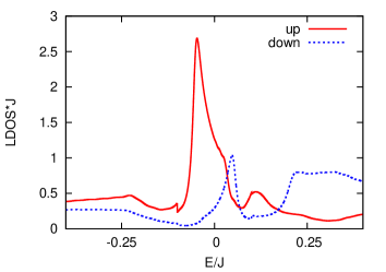
Figure 6: (Color online) LDOS at the surface of the system near the coexistence of the SC and AF states. The parameters are the same as those used in Fig. 4.

5 Summary and Discussion

We have studied the states near the (110) surfaces of $d_{x^{2}-y^{2}}$- wave superconductors that are described by the extended $t-J$ model. Since SC order is strongly suppressed there, the flux phase may occur and it can exist even for a large doping rate ($\delta\lesssim 0.20$), if the Fermi surface of the system is favorable to this state. Since the flux phase breaks ${\cal T}$, this may explain the results of experiments on the Kerr effect.[13, 14, 15] In the present theory, the ${\cal T}$ violation occurs only near the surface, and the surface states at the opposite sides of the sample are independent. Then it may give a simple explanation of the experimental finding that the signs of the Kerr angles at the opposite surfaces are the same.[15] The AF state may also appear near the (110) surface, and relative stability of the emergent surface states may be different from system to system depending on their FSs.

In this paper we did not consider the pseudogap phase (i.e., $T>T_{C}$ in the underdoped region). Experimentally, nonzero Kerr rotations are observed not only in the SC state but also in the pseudogap phase.[13, 14, 15] In order to understand this, we should include the dynamics of holons, and the effect of fluctuations around the SBMA solution ($U(1)$ gauge fluctuations) must be examined. Moreover, in experiments on the YBCO system, nonzero Kerr rotations are observed for doping rates higher than $\delta_{c}$ that we have obtained theoretically.[13] This could be due to the fact that we have treated only the single-layer (single-band) $t-J$ model. In bilayer or multilayer models, there are multiple FSs, and the condition for the occurrence of the flux phase and the AF state may be changed quantitatively. Whether this scenario is correct or not can be checked by carrying out similar calculations employing the bilayer $t-J$ model. This problem will be studied separately in the future.

The author thanks M. Hayashi, M. Mori, and H. Yamase for useful discussions. This work was supported by JSPS KAKENHI Grant Number 24540392.

References

- [1] H. Mukuda, S. Shimizu, A. Iyo, and Y. Kitaoka: J. Phys. Soc. Jpn. 81, 011008 (2012).
- [2] T. Timusk and B. Statt: Rep. Prog. Phys. 62, 61 (1999).
- [3] M. R. Norman, D. Pines, and C. Kallin, Adv. in Phys. 54, 715 (2005).
- [4] I. Affleck and J. B. Marston, Phys. Rev. B37, 3774 (1988).
- [5] For a review on the model, see M. Ogata and H. Fukuyama: Rep. Prog. Phys. 71, 036501 (2008).
- [6] S. Chakravarty, R. B. Laughlin, D. K. Morr, and C. Nayak: Phys. Rev. B63, 094503 (2001).
- [7] F. C. Zhang: Phys. Rev. Lett. 64 974 (1990).
- [8] K. Hamada and D. Yoshioka : Phys. Rev. B67, 184503 (2003).
- [9] M. Bejas, A. Greco, and H. Yamase: Phys. Rev. B86, 224509 (2012).
- [10] Z. Zou and P. W. Anderson: Phys. Rev. B37, 627 (1988).
- [11] P. A. Lee, N. Nagaosa, and X.-G. Wen: Rev. Mod. Phys. 78, 17 (2006).
- [12] K. Kuboki, J. Phys. Soc. Jpn. 83, 015003 (2014).
- [13] J. Xia, E. Schemm, G. Deutscher, S. A. Kivelson, D. A. Bonn, W. N. Hardy, R. Liang, W. Siemons, G. Koster, M. M. Fejer, and A. Kapitulnik: Phys. Rev. Lett. 100, 127002 (2008).
- [14] H. Karapetyan, M. Hücker, G. D. Gu, J. M. Tranquada, M. M. Fejer, J. Xia, and A. Kapitulnik, Phys. Rev. Lett. 109, 147001 (2012).
- [15] H. Karapetyan, J. Xia, M. Hucker, G. D. Gu, J. M. Tranquada, M.M. Fejer, A. Kapitulnik, Phys. Rev. Lett. 112, 047003 (2014).
- [16] S. Tewari, C. Zhang, V. M. Yakovenko, and S. Das Sarma, Phys. Rev. Lett. 100, 217004 (2008).
- [17] P. Hosur, A. Kapitulnik, S. A. Kivelson, J. Orenstein, and S. Raghu, Phys. Rev. B 87, 115116 (2013).
- [18] J. Orenstein and Joel E. Moore, Phys. Rev. B 87, 165110 (2013).
- [19] V. Aji, Y. He, and C. M. Varma, Phys. Rev. B 87, 174518 (2013).
- [20] S. S. Pershoguba, K. Kechedzhi, and V. M. Yakovenko, Phys. Rev. lett. 111, 047005 (2013).
- [21] B. Keimer, N. Belk, R. J. Birgeneau, A. Cassanho, C. Y. Chen, M. Greven, M. A. Kastner, A. Aharony, Y. Endoh, R. W. Erwin, and G. Shirane: Phys. Rev. B46, 14034 (1992).
- [22] S. Sanna, G. Allodi, G. Concas, A. D. Hillier, and R. De Renzi: Phys. Rev. Lett. 93, 207001 (2004).
- [23] P. G. de Gennes, Superconductivity of Metals and Alloys (Addison-Wesley, Reading, MA, 1989).
- [24] G. Kotliar and J. Liu, Phys. Rev. B 38, 5142 (1988).
- [25] Y. Suzumura, Y. Hasegawa, and H. Fukuyama, J. Phys. Soc. Jpn. 57, 2768 (1988).
- [26] M. Inaba, H. Matsukawa, M. Saitoh, and H. Fukuyama, Physica C 257, 299 (1996).
- [27] H. Yamase and H. Kohno, Phys. Rev. B69104526 (2004).
- [28] H. Yamase, M. Yoneya, and K. Kuboki, Phys. Rev. B84, 014508 (2011).
- [29] J. Brinckmann and P. A. Lee, Phys. Rev. Lett. 82, 2915 (1999).
- [30] H. Yamase, H. Kohno, H. Fukuyama, and M. Ogata, J. Phys. Soc.Jpn. 68, 1082 (1999).
- [31] G. C. Psaltakis and E. W. Fenton: J. Phys. C16 (1983) 3913.
- [32] M. Murakami and H. Fukuyama, J. Phys. Soc. Jpn. 67, 2784 (1998).
- [33] M. Murakami, J. Phys. Soc. Jpn. 69, 1113 (2000).
- [34] B. Kyung, Phys. Rev. B62, 9083 (2000).
- [35] A. Aperis, G. Varelogiannis, P. B. Littlewood, and B. D. Simons, J. Phys.: Condens. Matter 20, 434235 (2008).
- [36] K. Kuboki, J. Phys. Soc. Jpn. 68, 3150 (1999).
- [37] Y. Tanuma, Y. Tanaka, M. Ogata, and S. Kashiwaya, Phys. Rev. B 60, 9817 (1999).
- [38] J. X. Zhu and C. S. Ting, Phys. Rev. B 61, 1456 (2000).
- [39] K. Kuboki and H. Takahashi, Phys. Rev. B 70, 214524 (2004).
- [40] T. Tanamoto, H. Kohno, and H. Fukuyama, J. Phys. Soc. Jpn. 61, 1886 (1992).
- [41] K. Kuboki, J. Phys. Soc. Jpn 82, 014701 (2013).
- [42] M. Sigrist and K. Ueda, Rev. Mod. Phys. 63, 239 (1991).
- [43] M. Covington, M. Aprili, E. Paraoanu, L. H. Greene, F. Xu, J. Zhu, and C. A. Mirkin, Phys. Rev. Lett. 79, 277 (1997).
- [44] M. Fogelström, D. Rainer, and J. A. Sauls, Phys. Rev. Lett. 79, 281 (1997).